Как вставить символ юникода в excel

С помощью кодировок символов ASCII и Юникода можно хранить данные на компьютере и обмениваться ими с другими компьютерами и программами. Ниже перечислены часто используемые латинские символы ASCII и Юникода. Наборы символов Юникода, отличные от латинских, можно посмотреть в соответствующих таблицах, упорядоченных по наборам.

В этой статье

• Вставка символа ASCII или Юникода в документ

• Коды часто используемых символов

• Коды часто используемых диакритических знаков

• Коды часто используемых лигатур

• Непечатаемые управляющие знаки ASCII

• Дополнительные сведения

Вставка символа ASCII или Юникода в документ

Если вам нужно ввести только несколько специальных знаков или символов, можно использовать таблицу символов или сочетания клавиш. Список символов ASCII см. в следующих таблицах или статье Вставка букв национальных алфавитов с помощью сочетаний клавиш.

Примечания: 

• Многие языки содержат символы, которые не удалось уплотить в расширенный набор ACSII, содержащий 256 символов. Таким образом, существуют варианты ASCII и Юникода, которые включают региональные символы и символы. См. таблицы кодов символов Юникода по сценариям.

• Если у вас возникают проблемы с вводом кода необходимого символа, попробуйте использовать таблицу символов.

Вставка символов ASCII

Чтобы вставить символ ASCII, нажмите и удерживайте клавишу ALT, вводя код символа. Например, чтобы вставить символ градуса (º), нажмите и удерживайте клавишу ALT, затем введите 0176 на цифровой клавиатуре.

Для ввода чисел используйте цифровую клавиатуру, а не цифры на основной клавиатуре. Если на цифровой клавиатуре необходимо ввести цифры, убедитесь, что включен индикатор NUM LOCK.

Вставка символов Юникода

Чтобы вставить символ Юникода, введите код символа, затем последовательно нажмите клавиши ALT и X. Например, чтобы вставить символ доллара ($), введите 0024 и последовательно нажмите клавиши ALT и X. Все коды символов Юникода см. в таблицах символов Юникода, упорядоченных по наборам.

Важно: Некоторые программы Microsoft Office, например PowerPoint и InfoPath, не поддерживают преобразование кодов Юникода в символы. Если вам необходимо вставить символ Юникода в одной из таких программ, используйте таблицу символов.

Примечания: 

• Если после нажатия клавиш ALT+X отображается неправильный символ Юникода, выберите правильный код, а затем снова нажмите ALT+X.

• Кроме того, перед кодом следует ввести «U+».  Например, если ввести «1U+B5» и нажать клавиши ALT+X, отобразится текст «1µ», а если ввести «1B5» и нажать клавиши ALT+X, отобразится символ «Ƶ».

Использование таблицы символов

Таблица символов — это программа, встроенная в Microsoft Windows, которая позволяет просматривать символы, доступные для выбранного шрифта.

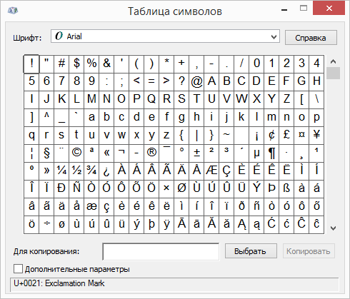
С помощью таблицы символов можно копировать отдельные символы или группу символов в буфер обмена и вставлять их в любую программу, поддерживающую отображение этих символов. Открытие таблицы символов

• В Windows 10 Введите слово «символ» в поле поиска на панели задач и выберите таблицу символов в результатах поиска.

• В Windows 8 Введите слово «символ» на начальном экране и выберите таблицу символов в результатах поиска.

• В Windows 7: Нажмите кнопку Пуск, а затем последовательно выберите команды Программы, Стандартные, Служебные и Таблица знаков.

Символы группются по шрифтам. Щелкните список шрифтов, чтобы выбрать набор символов. Чтобы выбрать символ, щелкните его, нажмите кнопку Выбрать, щелкните правой кнопкой мыши место в документе, в котором он должен быть, а затем выберите в документе кнопку Вировать.

К началу страницы

Коды часто используемых символов

Полный список символов см. в таблице символов на компьютере, таблице кодов символов ASCII или таблицах символов Юникода, упорядоченных по наборам.

Глиф	Код	Глиф	Код
Денежные единицы
£	ALT+0163	¥	ALT+0165
¢	ALT+0162	$	0024+ALT+X
€	ALT+0128	¤	ALT+0164
Юридические символы
©	ALT+0169	®	ALT+0174
§	ALT+0167	™	ALT+0153
Математические символы
°	ALT+0176	º	ALT+0186
√	221A+ALT+X	+	ALT+43
#	ALT+35	µ	ALT+0181
<	ALT+60	>	ALT+62
%	ALT+37	(	ALT+40
[	ALT+91	)	ALT+41
]	ALT+93	∆	2206+ALT+X
Дроби
¼	ALT+0188	½	ALT+0189
		¾	ALT+0190
Знаки пунктуации и диалектные символы
?	ALT+63	¿	ALT+0191
!	ALT+33	‼	203+ALT+X
—	ALT+45	‘	ALT+39
«	ALT+34	,	ALT+44
.	ALT+46	|	ALT+124
/	ALT+47		ALT+92
`	ALT+96	^	ALT+94
«	ALT+0171	»	ALT+0187
«	ALT+174	»	ALT+175
~	ALT+126	&	ALT+38
:	ALT+58	{	ALT+123
;	ALT+59	}	ALT+125
Символы форм
□	25A1+ALT+X	√	221A+ALT+X

К началу страницы

Коды часто используемых диакритических знаков

Полный список глифов и соответствующих кодов см. в таблице символов.

Глиф	Код		Глиф	Код
Ã	ALT+0195		å	ALT+0229
Å	ALT+143		å	ALT+134
Ä	ALT+142		ä	ALT+132
À	ALT+0192		à	ALT+133
Á	ALT+0193		á	ALT+160
Â	ALT+0194		â	ALT+131
Ç	ALT+128		ç	ALT+135
Č	010C+ALT+X		č	010D+ALT+X
É	ALT+144		é	ALT+130
È	ALT+0200		è	ALT+138
Ê	ALT+202		ê	ALT+136
Ë	ALT+203		ë	ALT+137
Ĕ	0114+ALT+X		ĕ	0115+ALT+X
Ğ	011E+ALT+X		ğ	011F+ALT+X
Ģ	0122+ALT+X		ģ	0123+ALT+X
Ï	ALT+0207		ï	ALT+139
Î	ALT+0206		î	ALT+140
Í	ALT+0205		í	ALT+161
Ì	ALT+0204		ì	ALT+141
Ñ	ALT+165		ñ	ALT+164
Ö	ALT+153		ö	ALT+148
Ô	ALT+212		ô	ALT+147
Ō	014C+ALT+X		ō	014D+ALT+X
Ò	ALT+0210		ò	ALT+149
Ó	ALT+0211		ó	ALT+162
Ø	ALT+0216		ø	00F8+ALT+X
Ŝ	015C+ALT+X		ŝ	015D+ALT+X
Ş	015E+ALT+X		ş	015F+ALT+X
Ü	ALT+154		ü	ALT+129
Ū	ALT+016A		ū	016B+ALT+X
Û	ALT+0219		û	ALT+150
Ù	ALT+0217		ù	ALT+151
Ú	00DA+ALT+X		ú	ALT+163
Ÿ	0159+ALT+X		ÿ	ALT+152

К началу страницы

Коды часто используемых лигатур

Дополнительные сведения о лигатурах см. в статье Лигатура (соединение букв). Полный список лигатур и соответствующих кодов см. в таблице символов.

Глиф	Код		Глиф	Код
Æ	ALT+0198		æ	ALT+0230
ß	ALT+0223		ß	ALT+225
Œ	ALT+0140		œ	ALT+0156
			ʩ	02A9+ALT+X
ʣ	02A3+ALT+X		ʥ	02A5+ALT+X
ʪ	02AA+ALT+X		ʫ	02AB+ALT+X
ʦ	0246+ALT+X		ʧ	02A7+ALT+X
Љ	0409+ALT+X		Ю	042E+ALT+X
Њ	040A+ALT+X		Ѿ	047E+ALT+x
Ы	042B+ALT+X		Ѩ	0468+ALT+X
Ѭ	049C+ALT+X		ﷲ	FDF2+ALT+X

К началу страницы

Непечатаемые управляющие знаки ASCII

Знаки, используемые для управления некоторыми периферийными устройствами, например принтерами, в таблице ASCII имеют номера 0–31. Например, знаку перевода страницы/новой страницы соответствует номер 12. Этот знак указывает принтеру перейти к началу следующей страницы.

Таблица непечатаемых управляющих знаков ASCII

Десятичное число	Знак		Десятичное число	Знак
NULL	0		Освобождение канала данных	16
Начало заголовка	1		Первый код управления устройством	17
Начало текста	2		Второй код управления устройством	18
Конец текста	3		Третий код управления устройством	19
Конец передачи	4		Четвертый код управления устройством	20
Запрос	5		Отрицательное подтверждение	21
Подтверждение	6		Синхронный режим передачи	22
Звуковой сигнал	7		Конец блока передаваемых данных	23
BACKSPACE	8		Отмена	24
Горизонтальная табуляция	9		Конец носителя	25
Перевод строки/новая строка	10		Символ замены	26
Вертикальная табуляция	11		ESC	27
Перевод страницы/новая страница	12		Разделитель файлов	28
Возврат каретки	13		Разделитель групп	29
Сдвиг без сохранения разрядов	14		Разделитель записей	30
Сдвиг с сохранением разрядов	15		Разделитель данных	31
Пробел	32		DEL	127

К началу страницы

Дополнительные сведения

• Коды символов ASCII

• Клавиатура (иврит)

• Вставка букв национальных алфавитов с помощью сочетаний клавиш

• Вставка флажка или другого символа

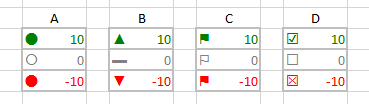
Special character symbols from the set of Unicode characters like ☐, ☑, ⚐, ⚑, ▲, and ▼ can be useful for many different things in Excel. You can use them in drop-down lists, charts, custom number formats, dot plots and in-cell pictographs. As the Office software and web browsers continue to support the display of more symbols, I expect the use of special characters will make it possible to do even more cool stuff with Excel.

I created this page so that I would have a quick reference for the types of symbols that I use frequently in Excel. Why? Because the Insert Symbol feature in Excel doesn’t include many of the symbols I like to use, and one of the easy ways to get a symbol into Excel is to copy/paste the symbol from a web page.

How to Insert a Symbol in Excel

1. From the Web: Copy and Paste

There are many places on the internet to find lists of unicode characters. Do a google search for «unicode …». Usually, you can just select the unicode character from your browser and press Ctrl+c to copy it, then Ctrl+v to paste it into Excel. If you are editing the text or formula within a cell, then it will paste just the character (instead of the formatting from the web page).

My favorite searchable resource for seeing what emojis look like in other software is unicode.org

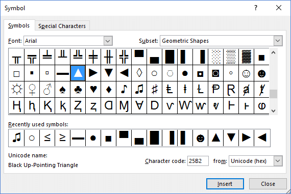
2. Excel: Insert > Symbol

You can browse some of the unicode characters using the Insert > Symbol dialog. It will tell you the name of the symbol as well as the character code.

The Insert Symbol Tool in Excel 2016

IMPORTANT: The Arial font doesn’t list many Unicode symbols, so change the Font to «Segoe UI Symbol» then in the Subset dropdown, select «Miscellaneous Symbols» and start scrolling down. Unfortunately, there isn’t a good search feature to find what you want.

You can use the hexidecimal Character code value to display a character in html by entering it as &#xNNNN; where NNNN is the hex code. Example: ▲ (▲)

If you have found the Decimal code (which I have listed on this page for many symbols), you display it in html as &#NNNN; (leaving out the «x»).

3. Windows: Inserting Special Symbols Using ALT Codes

Some special characters can be inserted by pressing ALT+#, where the # is entered using the number pad. Hold the Alt key while you press the number sequence then lift up on the ALT key. I’ve only learned one code by heart: ALT+0169 is the © symbol. See the references below for a list of ALT codes.

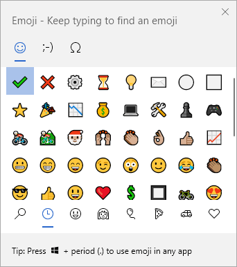
4. Windows 10: Emoji Keyboard Panel

The new Windows 10 update added a way to insert emojis from the keyboard. Open the Emoji Keyboard Panel by pressing ⊞ Win+. (Window key + Period) or ⊞ Win+;.

The Insert Symbol Tool in Excel 2016

I use this a LOT (only took a dozen or so times before I had the shortcut memorized), and you can see from my screenshot which emojis I use most recently. ✔ 🙂

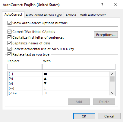
5. Excel: Create Shortcuts to Insert Symbols Using Auto-Correct

You may already be familiar with how (c) automatically changes to © and (r) changes to ® in Office applications. When using this feature, you type (c) and then either press Enter or another character, and Excel changes it to ©. If you don’t want that to happen, you can press Ctrl+z to undo the auto-correct.

The cool thing is that you can add your own custom shortcuts for the special characters or symbols that you use the most.

In Excel 2013/2016, go to File > Options > Proofing and click on Auto-correct Options. A window will pop that lets you define shortcuts for special symbols. I’ve been doing this for years, and have found that using the abbreviated name or graphical representation in parentheses works great. For example (plusmn) for ±, and (middot) for the dot you place between units in labels like N·m (Newton-meter).

Files > Options > Proofing > Autocorrect Options

The table below lists only SOME of the thousands of symbols you might want to use. Some of the names in parentheses are the same named used for the HTML equivalent, such as ° for ° and ÷ for ÷. Others are just examples of what I like to use such as (->>) for ►.

(plusmn)	±	(alpha)	α	(capalpha)	Α	(/)	▲
(deg)	°	(beta)	β	(capbeta)	Β	(/)	▼
(micro)	µ	(gamma)	γ	(capgamma)	Γ	(<<-)	◄
(ohm)	Ω	(delta)	δ	(capdelta)	Δ	(->>)	►
(infin)	∞	(epsilon)	ε	(capepsilon)	Ε	(—)	▬
(middot)	·	(zeta)	ζ	(capzeta)	Ζ	(larr)	←
(bull)	•	(eta)	η	(capeta)	Η	(rarr)	→
(ge)	≥	(theta)	θ	(captheta)	Θ	(uarr)	↑
(le)	≤	(kappa)	κ	(capkappa)	Κ	(darr)	↓
(ne)	≠	(lambda)	λ	(caplambda)	Λ	(star)	★
(asymp)	≈	(mu)	μ	(capmu)	Μ	(starempty)	☆
(dot)	˙	(xi)	ξ	(capxi)	Ξ	(heart)	❤
(equiv)	≡	(pi)	π	(cappi)	Π	(lightcheck)	✓
(part)	∂	(rho)	ρ	(caprho)	Ρ	(check)	✔
(change)	∆	(tau)	τ	(captau)	Τ	(boxE)	☐
(del)	∇	(omega)	ω	(capomega)	Ω	(boxC)	☑
(times)	×	(sigma)	σ	(capsigma)	Σ	(boxX)	☒
(divide)	÷	(phi)	φ	(capphi)	Φ	(lightmark)	✗
(radic)	√	(circ)	⬤	(block)	█	(mark)	✘
(sum)	∑	(circempty)	◯	(smallblock)	▇	(flag)	⚑
(prod)	∏	(cut)	✁	(note)	♪	(flagempty)	⚐

Using the UNICHAR and UNICODE functions

The UNICODE and UNICHAR functions have been available since Excel 2013 and are similar to the older CODE and CHAR functions.

The UNICHAR function is perhaps the most useful, because it will return the character for a given decimal value (UTF-8 and UTF-16), like this:

=UNICHAR(10004)        returns ✔

The UNICODE function does the reverse. It returns the numeric decimal Unicode value for the first character in a text string, like this:

=UNICODE("✔")        returns 10004

If you want to try something fancy, you can use the following array formula (press Ctrl+Shift+Enter after entering an array formula) to return an array of Unicode values for each of the characters in a text string.

=UNICODE(MID(text_string,ROW(INDIRECT("1:"&LEN(text_string))),1))

Symbols in Data Validation Drop-Downs

Using special symbols or dingbats within drop-down lists is a great substitute for a checkbox in Excel. I’ve demonstrated this in various task list and action item templates. You can also use stars or flag symbols for flagging priority items in a list.

Try It — Create a Substitute for a Checkbox in Excel: Open a new worksheet in Excel, select cell A1 then go to Data > Data Validation and select the List option. Copy the following characters (including the comma), and paste them into the Source field: ☐, ☑

Check Marks and Check Boxes

✓ 10003

✔ 10004

✕ 10005

✖ 10006

✗ 10007

✘ 10008

☐ 9744

☑ 9745

☒ 9746

Flags and Circles

⚑ 9873

⚐ 9872

⬤ 11044

ⵔ 11604

◯ 9711

🏁 127937

🏴 127988

🚩 128681

Symbols for Milestones

Symbols for Priorities

🔥 128293 hot

❆ 10054 cold

♨ 9832 warm

See the CRM Template for an example of how these symbols are used.

Symbols for Ratings

★ 9733

☆ 9734

❤ 10084

♥ 9829

♡ 9825

👍 128077

👎 128078

The feature comparison template demonstrates how you can use a data validation drop-down list to create a star-rating by entering ★,★★,★★★ into the Source box for the list.

Emoji Rating System

😍 128525

😃 128515

🙂 128578

😐 128528

😕 128533

🙁 128577

😠 128544

For a larger list of emoticons, see this page.

Data Bars and Pictographs

Pictographs or Dot Plots

You can use the =REPT(text,number_times) function to repeat a character, as demonstrated in the article «Create a Dot Plot in Excel». Below is an example of a very basic in-cell pictograph.

In-Cell Dot Plot using REPT

One of the problems with using symbols for pictographs is that the REPT() function cannot display a fraction of a symbol. If you need a graph to show decimal values rather than just whole numbers, you can create a small picture (such as a screen capture of a Unicode character) and use it within an Excel chart to create a pictograph like the example below.

Sample Pictograph in Excel using a Bar Chart and Picture Fill

Data Bars

Data bars are often used in spreadsheet dashboards to show in-cell bar graphs. They can also be used for progress bars if the cell is scaled to 0%-100%. You may not need to use this technique for in-cell graphics in Excel any more because of the awesome conditional formatting options. However, Google Sheets does not have in-cell data bars yet, so using the REPT() function is one way to create something like a data bar (see the image below).

Data Bar in Google Sheets

The table below lists the main characters I use for this technique. Note that although there are some skinny bars (like 9612), for data bars you need to use the characters that do not include any blank space.

▆ 9606	▇ 9607	█ 9608	▌ 9612
▆▆▆▆	▇▇▇▇	████	▌▌▌▌

Sprint Progress Charts

What I call a «sprint chart» or «sprint progress chart» is a simple graph that shows progress relative to the amount of time left. This technique can be useful as a visual aid in Agile Product Development. Download the Kanban Board Template to see it in action. The «sprint» period is represented as a number of days, with a flag for each day. The filled-in flags ⚑ represent the percent completed and the watch or hourglass symbol represents the current day. The example chart below is showing multiple teams’ race against time.

A Sprint Progress Chart Using the REPT Function

Here is the formula for creating the in-cell sprint chart:

sprint = 14   (# of days in the sprint)
progress = 34.5%
complete = ROUND(sprint*progress,0)
time = IF(TODAY()<start_date,0,IF(TODAY()>(start_date+sprint),sprint,TODAY()-start_date))

=REPT("⚑",MIN(time,complete)) & REPT("⚐",MAX(0,time-complete)) & "⌛" & REPT("⚑",MAX(0,complete-time)) & REPT("⚐",sprint-MAX(time,complete)) & "🏁"

Other Useful Symbols

Triangles / Arrows

▬ 9644	▲ 9650	▼ 9660	► 9658	◄ 9668
ALT+22	ALT+30	ALT+31	ALT+16	ALT+17

These are the symbols I like to use for up/down signals. The dash is obviously not an arrow, but the this dash symbol works well as a «zero» when using the up/down symbols in custom number formats (see the examples below). There are a LOT of different kinds of arrows, but I use these triangles more often than other arrows. See my Unicode Symbols page for a huge list of arrows.

Scissors

✀ 9984	✁ 9985	✂ 9986	✃ 9987
✁——————————

In combination with a custom number format of «@*-» and merged cells, the scissors can be used in forms like a remittance slip on a billing invoice to create a guide for cutting.

Some Sports Symbols

⚽ 9917

⚾ 9918

🏈 127944

🏀 127936

🚲 128690

⛳ 9971

🎾 127934

⛷ 9975

⛸ 9976

Time and Clocks

⌚ 8986

⏰ 9200

⌛ 8987

⏳ 9203

🕓 128339

🕜 128348

There are symbols for each hour and half hour on the clock. See this page for a full list.

Moon Phases

🌑 127761

🌒 127762

🌓 127763

🌔 127764

🌕 127765

🌖 127766

🌗 127767

🌘 127768

🌙 127769

These symbols can be used to create a Moon Phase Calendar in Excel. The template I created uses the symbols within conditional formatting rules and custom number formats.

Symbols in Custom Number Formats

Special characters can be used within custom number formats as a substitute for conditional formatting icons. You can also use this technique to format numbers that appear in charts! Take a look at the examples below.

Examples using custom number formats with special symbols

The following custom format codes were used to generate the example shown in the screenshot above:

⬤,ⵔ : [Color10]⬤* 0;[Red]⬤* -0;[Color16]ⵔ* 0;@
▲,▬,▼ : [Color10]▲* 0;[Red]▼* -0;[Color16]▬* 0;@
⚑,⚐ : [Color10]⚑* 0;[Red]⚑* -0;[Color16]⚐* 0;@
☑,☐,☒ : [Color10]☑* 0;[Red]☒* -0;[Color16]☐* 0;@

If you haven’t seen color codes like [ColorN] used in custom number formats before, you can read this article. I created the graphic below to show how the [ColorN] codes correlate to the the old .xls color palette. I created the squares (█▌) next to the color codes by combining the █ and ▌ characters.

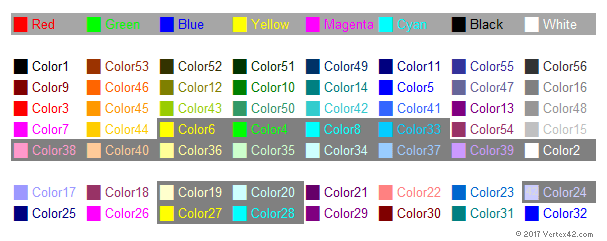Color codes for custom number formats (based on the default color palette)

Examples in Templates

1. Feature Comparison Template — This template demonstrates many different ways of using unicode characters and conditional formatting, including check boxes and star-ratings within drop-downs.

✓, ✔, 🗶, ✗, ✘, ✪, ★, ☐, ☑, ☒, ⚐, ⚑, ◆, ⬧

★,★★,★★★,★★★★,★★★★★

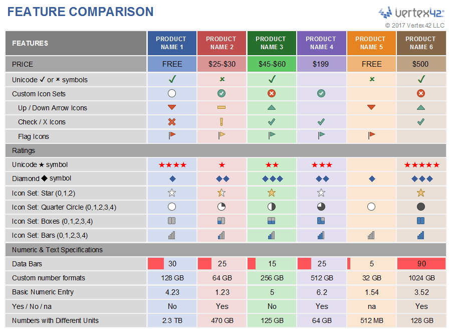
2. Attendance Sheet Template — This template shows how you can use fun symbols for taking attendance instead of a boring «x». The COUNTA() function will count the cells that aren’t blank, so it doesn’t matter what symbol you use. These characters look even better in the Excel app on an iPhone.

3. Blood Sugar Chart Template — You can add some fun to perhaps an otherwise boring chart or log by adding emojis within drop-down lists (and even in the chart itself, by using screenshot images of emojis as data point markers).

Emojis, Emoticons, and other Miscellaneous Symbols

The Unicode emojis and emoticons do not necessarily appear the same in all browsers and apps, but it’s worth pointing out that most of these symbols can be displayed in new versions of Excel. The following table provides a quick way to look at some of these symbols. To browse a huge list of Unicode symbols, see my Unicode Symbols page.

To use one of these characters in Excel: you can copy/paste a character from the table below. After copying the emoji character, you can paste it within a formula or anywhere else that you might paste a text character.

😀 128512	😁 128513	😂 128514	😃 128515	😄 128516	😅 128517	😆 128518	😇 128519	😈 128520	😉 128521	😊 128522	😋 128523
😌 128524	😍 128525	😎 128526	😏 128527	😐 128528	😑 128529	😒 128530	😓 128531	😔 128532	😕 128533	😖 128534	😗 128535
😘 128536	😙 128537	😚 128538	😛 128539	😜 128540	😝 128541	😞 128542	😟 128543	😠 128544	😡 128545	😢 128546	😣 128547
😤 128548	😥 128549	😦 128550	😧 128551	😨 128552	😩 128553	😪 128554	😫 128555	😬 128556	😭 128557	😮 128558	😯 128559
😰 128560	😱 128561	😲 128562	😳 128563	😴 128564	😵 128565	😶 128566	😷 128567	😸 128568	😹 128569	😺 128570	😻 128571
😼 128572	😽 128573	😾 128574	😿 128575	🙀 128576	🙁 128577	🙂 128578	🙃 128579	🙄 128580	🙅 128581	🙆 128582	🙇 128583
🙈 128584	🙉 128585	🙊 128586	🙋 128587	🙌 128588	🙍 128589	🙎 128590	🙏 128591
🚀 128640	🚁 128641	🚂 128642	🚃 128643	🚄 128644	🚅 128645	🚆 128646	🚇 128647	🚈 128648	🚉 128649	🚊 128650	🚋 128651
🚌 128652	🚍 128653	🚎 128654	🚏 128655	🚐 128656	🚑 128657	🚒 128658	🚓 128659	🚔 128660	🚕 128661	🚖 128662	🚗 128663
🚘 128664	🚙 128665	🚚 128666	🚛 128667	🚜 128668	🚝 128669	🚞 128670	🚟 128671	🚠 128672	🚡 128673	🚢 128674	🚣 128675
🚤 128676	🚥 128677	🚦 128678	🚧 128679	🚨 128680	🚩 128681	🚪 128682	🚫 128683	🚬 128684	🚭 128685	🚮 128686	🚯 128687
🚰 128688	🚱 128689	🚲 128690	🚳 128691	🚴 128692	🚵 128693	🚶 128694	🚷 128695	🚸 128696	🚹 128697	🚺 128698	🚻 128699
🚼 128700	🚽 128701	🚾 128702	🚿 128703	🛀 128704	🛁 128705	🛂 128706	🛃 128707	🛄 128708	🛅 128709	🛆 128710	🛇 128711
🛈 128712	🛉 128713	🛊 128714	🛋 128715	🛌 128716	🛍 128717	🛎 128718	🛏 128719	🛐 128720	🛑 128721	🛒 128722	🛓 128723
🛠 128736	🛡 128737	🛢 128738	🛣 128739	🛤 128740	🛥 128741	🛦 128742	🛧 128743	🛨 128744	🛩 128745	🛪 128746	🛫 128747
🛬 128748	🛭 128749	🛮 128750	🛯 128751	🛰 128752	🛱 128753	🛲 128754	🛳 128755	🛴 128756	🛵 128757	🛶 128758	🛷 128759
🌀 127744	🌁 127745	🌂 127746	🌃 127747	🌄 127748	🌅 127749	🌆 127750	🌇 127751	🌈 127752	🌉 127753	🌊 127754	🌋 127755
🌌 127756	🌍 127757	🌎 127758	🌏 127759	🌐 127760	🌑 127761	🌒 127762	🌓 127763	🌔 127764	🌕 127765	🌖 127766	🌗 127767
🌘 127768	🌙 127769	🌚 127770	🌛 127771	🌜 127772	🌝 127773	🌞 127774	🌟 127775	🌠 127776	🌡 127777	🌢 127778	🌣 127779
🌤 127780	🌥 127781	🌦 127782	🌧 127783	🌨 127784	🌩 127785	🌪 127786	🌫 127787	🌬 127788	🌭 127789	🌮 127790	🌯 127791
🌰 127792	🌱 127793	🌲 127794	🌳 127795	🌴 127796	🌵 127797	🌶 127798	🌷 127799	🌸 127800	🌹 127801	🌺 127802	🌻 127803
🌼 127804	🌽 127805	🌾 127806	🌿 127807	🍀 127808	🍁 127809	🍂 127810	🍃 127811	🍄 127812	🍅 127813	🍆 127814	🍇 127815
🍈 127816	🍉 127817	🍊 127818	🍋 127819	🍌 127820	🍍 127821	🍎 127822	🍏 127823	🍐 127824	🍑 127825	🍒 127826	🍓 127827
🍔 127828	🍕 127829	🍖 127830	🍗 127831	🍘 127832	🍙 127833	🍚 127834	🍛 127835	🍜 127836	🍝 127837	🍞 127838	🍟 127839
🍠 127840	🍡 127841	🍢 127842	🍣 127843	🍤 127844	🍥 127845	🍦 127846	🍧 127847	🍨 127848	🍩 127849	🍪 127850	🍫 127851
🍬 127852	🍭 127853	🍮 127854	🍯 127855	🍰 127856	🍱 127857	🍲 127858	🍳 127859	🍴 127860	🍵 127861	🍶 127862	🍷 127863
🍸 127864	🍹 127865	🍺 127866	🍻 127867	🍼 127868	🍽 127869	🍾 127870	🍿 127871	🎀 127872	🎁 127873	🎂 127874	🎃 127875
🎄 127876	🎅 127877	🎆 127878	🎇 127879	🎈 127880	🎉 127881	🎊 127882	🎋 127883	🎌 127884	🎍 127885	🎎 127886	🎏 127887
🎐 127888	🎑 127889	🎒 127890	🎓 127891	🎔 127892	🎕 127893	🎖 127894	🎗 127895	🎘 127896	🎙 127897	🎚 127898	🎛 127899
🎜 127900	🎝 127901	🎞 127902	🎟 127903	🎠 127904	🎡 127905	🎢 127906	🎣 127907	🎤 127908	🎥 127909	🎦 127910	🎧 127911
🎨 127912	🎩 127913	🎪 127914	🎫 127915	🎬 127916	🎭 127917	🎮 127918	🎯 127919	🎰 127920	🎱 127921	🎲 127922	🎳 127923
🎴 127924	🎵 127925	🎶 127926	🎷 127927	🎸 127928	🎹 127929	🎺 127930	🎻 127931	🎼 127932	🎽 127933	🎾 127934	🎿 127935
🏀 127936	🏁 127937	🏂 127938	🏃 127939	🏄 127940	🏅 127941	🏆 127942	🏇 127943	🏈 127944	🏉 127945	🏊 127946	🏋 127947
🏌 127948	🏍 127949	🏎 127950	🏏 127951	🏐 127952	🏑 127953	🏒 127954	🏓 127955	🏔 127956	🏕 127957	🏖 127958	🏗 127959
🏘 127960	🏙 127961	🏚 127962	🏛 127963	🏜 127964	🏝 127965	🏞 127966	🏟 127967	🏠 127968	🏡 127969	🏢 127970	🏣 127971
🏤 127972	🏥 127973	🏦 127974	🏧 127975	🏨 127976	🏩 127977	🏪 127978	🏫 127979	🏬 127980	🏭 127981	🏮 127982	🏯 127983
🏰 127984	🏱 127985	🏲 127986	🏳 127987	🏴 127988	🏵 127989	🏶 127990	🏷 127991	🏸 127992	🏹 127993	🏺 127994	🏻 127995
🏼 127996	🏽 127997	🏾 127998	🏿 127999	🐀 128000	🐁 128001	🐂 128002	🐃 128003	🐄 128004	🐅 128005	🐆 128006	🐇 128007
🐈 128008	🐉 128009	🐊 128010	🐋 128011	🐌 128012	🐍 128013	🐎 128014	🐏 128015	🐐 128016	🐑 128017	🐒 128018	🐓 128019
🐔 128020	🐕 128021	🐖 128022	🐗 128023	🐘 128024	🐙 128025	🐚 128026	🐛 128027	🐜 128028	🐝 128029	🐞 128030	🐟 128031
🐠 128032	🐡 128033	🐢 128034	🐣 128035	🐤 128036	🐥 128037	🐦 128038	🐧 128039	🐨 128040	🐩 128041	🐪 128042	🐫 128043
🐬 128044	🐭 128045	🐮 128046	🐯 128047	🐰 128048	🐱 128049	🐲 128050	🐳 128051	🐴 128052	🐵 128053	🐶 128054	🐷 128055
🐸 128056	🐹 128057	🐺 128058	🐻 128059	🐼 128060	🐽 128061	🐾 128062	🐿 128063	👀 128064	👁 128065	👂 128066	👃 128067
👄 128068	👅 128069	👆 128070	👇 128071	👈 128072	👉 128073	👊 128074	👋 128075	👌 128076	👍 128077	👎 128078	👏 128079
👐 128080	👑 128081	👒 128082	👓 128083	👔 128084	👕 128085	👖 128086	👗 128087	👘 128088	👙 128089	👚 128090	👛 128091
👜 128092	👝 128093	👞 128094	👟 128095	👠 128096	👡 128097	👢 128098	👣 128099	👤 128100	👥 128101	👦 128102	👧 128103
👨 128104	👩 128105	👪 128106	👫 128107	👬 128108	👭 128109	👮 128110	👯 128111	👰 128112	👱 128113	👲 128114	👳 128115
👴 128116	👵 128117	👶 128118	👷 128119	👸 128120	👹 128121	👺 128122	👻 128123	👼 128124	👽 128125	👾 128126	👿 128127
💀 128128	💁 128129	💂 128130	💃 128131	💄 128132	💅 128133	💆 128134	💇 128135	💈 128136	💉 128137	💊 128138	💋 128139
💌 128140	💍 128141	💎 128142	💏 128143	💐 128144	💑 128145	💒 128146	💓 128147	💔 128148	💕 128149	💖 128150	💗 128151
💘 128152	💙 128153	💚 128154	💛 128155	💜 128156	💝 128157	💞 128158	💟 128159	💠 128160	💡 128161	💢 128162	💣 128163
💤 128164	💥 128165	💦 128166	💧 128167	💨 128168	💩 128169	💪 128170	💫 128171	💬 128172	💭 128173	💮 128174	💯 128175
💰 128176	💱 128177	💲 128178	💳 128179	💴 128180	💵 128181	💶 128182	💷 128183	💸 128184	💹 128185	💺 128186	💻 128187
💼 128188	💽 128189	💾 128190	💿 128191	📀 128192	📁 128193	📂 128194	📃 128195	📄 128196	📅 128197	📆 128198	📇 128199
📈 128200	📉 128201	📊 128202	📋 128203	📌 128204	📍 128205	📎 128206	📏 128207	📐 128208	📑 128209	📒 128210	📓 128211
📔 128212	📕 128213	📖 128214	📗 128215	📘 128216	📙 128217	📚 128218	📛 128219	📜 128220	📝 128221	📞 128222	📟 128223
📠 128224	📡 128225	📢 128226	📣 128227	📤 128228	📥 128229	📦 128230	📧 128231	📨 128232	📩 128233	📪 128234	📫 128235
📬 128236	📭 128237	📮 128238	📯 128239	📰 128240	📱 128241	📲 128242	📳 128243	📴 128244	📵 128245	📶 128246	📷 128247
📸 128248	📹 128249	📺 128250	📻 128251	📼 128252	📽 128253	📾 128254	📿 128255	🔀 128256	🔁 128257	🔂 128258	🔃 128259
🔄 128260	🔅 128261	🔆 128262	🔇 128263	🔈 128264	🔉 128265	🔊 128266	🔋 128267	🔌 128268	🔍 128269	🔎 128270	🔏 128271
🔐 128272	🔑 128273	🔒 128274	🔓 128275	🔔 128276	🔕 128277	🔖 128278	🔗 128279	🔘 128280	🔙 128281	🔚 128282	🔛 128283
🔜 128284	🔝 128285	🔞 128286	🔟 128287	🔠 128288	🔡 128289	🔢 128290	🔣 128291	🔤 128292	🔥 128293	🔦 128294	🔧 128295
🔨 128296	🔩 128297	🔪 128298	🔫 128299	🔬 128300	🔭 128301	🔮 128302	🔯 128303	🔰 128304	🔱 128305	🔲 128306	🔳 128307
🔴 128308	🔵 128309	🔶 128310	🔷 128311	🔸 128312	🔹 128313	🔺 128314	🔻 128315	🔼 128316	🔽 128317	🔾 128318	🔿 128319
🕀 128320	🕁 128321	🕂 128322	🕃 128323	🕄 128324	🕅 128325	🕆 128326	🕇 128327	🕈 128328	🕉 128329	🕊 128330	🕋 128331
🕌 128332	🕍 128333	🕎 128334	🕏 128335	🕐 128336	🕑 128337	🕒 128338	🕓 128339	🕔 128340	🕕 128341	🕖 128342	🕗 128343
🕘 128344	🕙 128345	🕚 128346	🕛 128347	🕜 128348	🕝 128349	🕞 128350	🕟 128351	🕠 128352	🕡 128353	🕢 128354	🕣 128355
🕤 128356	🕥 128357	🕦 128358	🕧 128359	🕨 128360	🕩 128361	🕪 128362	🕫 128363	🕬 128364	🕭 128365	🕮 128366	🕯 128367
🕰 128368	🕱 128369	🕲 128370	🕳 128371	🕴 128372	🕵 128373	🕶 128374	🕷 128375	🕸 128376	🕹 128377	🕺 128378	🕻 128379
🕼 128380	🕽 128381	🕾 128382	🕿 128383	🖀 128384	🖁 128385	🖂 128386	🖃 128387	🖄 128388	🖅 128389	🖆 128390	🖇 128391
🖈 128392	🖉 128393	🖊 128394	🖋 128395	🖌 128396	🖍 128397	🖎 128398	🖏 128399	🖐 128400	🖑 128401	🖒 128402	🖓 128403
🖔 128404		🖖 128406	🖗 128407	🖘 128408	🖙 128409	🖚 128410	🖛 128411	🖜 128412	🖝 128413	🖞 128414	🖟 128415
🖠 128416	🖡 128417	🖢 128418	🖣 128419	🖤 128420	🖥 128421	🖦 128422	🖧 128423	🖨 128424	🖩 128425	🖪 128426	🖫 128427
🖬 128428	🖭 128429	🖮 128430	🖯 128431	🖰 128432	🖱 128433	🖲 128434	🖳 128435	🖴 128436	🖵 128437	🖶 128438	🖷 128439
🖸 128440	🖹 128441	🖺 128442	🖻 128443	🖼 128444	🖽 128445	🖾 128446	🖿 128447	🗀 128448	🗁 128449	🗂 128450	🗃 128451
🗄 128452	🗅 128453	🗆 128454	🗇 128455	🗈 128456	🗉 128457	🗊 128458	🗋 128459	🗌 128460	🗍 128461	🗎 128462	🗏 128463
🗐 128464	🗑 128465	🗒 128466	🗓 128467	🗔 128468	🗕 128469	🗖 128470	🗗 128471	🗘 128472	🗙 128473	🗚 128474	🗛 128475
🗜 128476	🗝 128477	🗞 128478	🗟 128479	🗠 128480	🗡 128481	🗢 128482	🗣 128483	🗤 128484	🗥 128485	🗦 128486	🗧 128487
🗨 128488	🗩 128489	🗪 128490	🗫 128491	🗬 128492	🗭 128493	🗮 128494	🗯 128495	🗰 128496	🗱 128497	🗲 128498	🗳 128499
🗴 128500	🗵 128501	🗶 128502	🗷 128503	🗸 128504	🗹 128505	🗺 128506	🗻 128507	🗼 128508	🗽 128509	🗾 128510	🗿 128511

Unicode Characters vs. Symbol/WingDings Fonts

One of the main benefits of using Unicode characters instead of Symbol and Wingdings fonts is that the Unicode characters will show up correctly in drop-down lists and you can use them in formulas and custom number formats. If you change the font of a cell to wingdings, the formula may still be readable in the Formula bar, but it is unreadable when editing the formula within the cell.

I’ve also had fewer compatibility problems when using common Unicode characters than when using special fonts.

Notes and References

✅, ❎ : Codes that are a specific color in a browser show as black/white in Excel desktop and the color can be changed. But changing the color of these won’t work in Excel online or Google Sheets, which are browser-based apps.

🙂,🙃,🙄,🙅,🙆,🙇,🙈,🙉 : Some emojis render the same way they appear in texts on the iPhone when used within the Excel mobile app.

Need to convert HEX codes to Decimal? Use the HEX2DEC() or DEC2HEX() functions in Excel.

References

• Unicode Characters at wikipedia.org
• The UNICHAR Function at support.office.com — The official syntax page.
• RapidTables.com Unicode Character Symbols at rapidtables.com — A useful place to browse the Unicode characters. Gives the HTML code and the Unicode.
• Alt Codes for Inserting Symbols at usefulshortcuts.com
• Conversion Utility for Using Special Symbols in CSS :before and :after
• History of Unicode at unicode.org
• Unicode Blocks at fileformat.info — lists blocks of symbols by category, including many of the newer symbols.

Problems can arise when converting the character codes from one system to another system. These problems result in garbled data. To correct this, a universal character set known as Unicode system was developed during the late 1980s that gives the characters used in computer systems a unique character code.

Thanks for letting us know!

Форматирование

04.04.2013 76230

Для кодирования символов в unicode в программе Excel используется функция UNICODE. Она предназначена для выполнения преобразования первого символа строки в соответствующее ему кодовое (числовое) значение согласно таблице стандарта кодировки Юникод, и возвращает соответствующее числовое значение.

Unicode – распространенный стандарт кодирования символов, содержащий символы практически всех языков мира. Является наиболее востребованным стандартом для сервисов в глобальной сети и программных продуктов, используемых на локальных устройствах.

Примеры использования функции UNICODE для кодирования символов в Excel

Пример 1. В таблице введены несколько букв русского алфавита. Необходимо в смежном столбце вывести численные представления указанных символов в кодировке Юникод.

Чтобы вывести сразу все значения, выделим ячейки B1:B7 и запишем следующую формулу, а для подтверждения нажмем комбинацию клавиш CTRL+Enter:

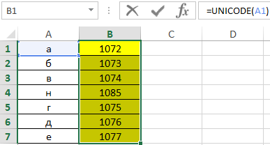
Как видно из данного примера в кодировке Юникод каждый символ букв кириллицы кодируется в четырехзначное число.



Кодирование и представление символов чисел и в кодировке Юникод

Пример 2. Вывести массив случайных чисел от 0 до 9, создать массив кодов Unicode для данных чисел. Определить, существует ли между ними взаимосвязь (визуально с помощью графика).

Вид таблицы со столбцом, заполненным случайными числами:

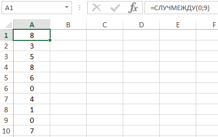
Для заполнения столбца была использована функция СЛУЧМЕЖДУ(0;9). При любом действии на листе Excel, данная функция выполняет пересчет значений. Чтобы получить статические данные, полученные числа были скопированы и вставлены в ячейки с использованием инструмента Специальная вставка -> значения.

Вычислим значения кодов Unicode с помощью формулы:

Построим график:

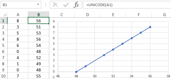
На основании данного графика можно сделать вывод: для больших значений чисел предусмотрены большие значения кодов, то есть нумерация в таблице Unicode идет последовательно для числовых значений (что, собственно, и так очевидно).

Посимвольное кодирование паролей в Excel

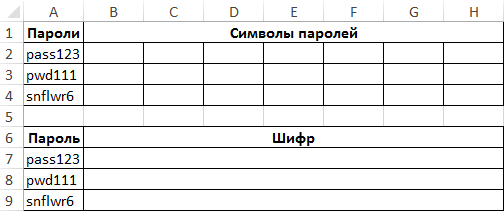
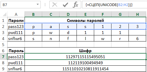
Пример 3. Создать простой способ шифрования пароля цифрами. В таблице есть несколько вариантов паролей, записать в смежном столбце их числовые шифры.

Вид таблицы данных:

Чтобы автоматизировать процедуру шифрования, необходима следующая логика:

1. Функция, выполняющая разбивку строки на отдельные символы.
2. При переборе каждого символа из массива выполняется преобразование в числовое представление Юникод.
3. Формирование новой строки из численных представлений символов.

Для такой задачи рационально использовать макросы VBA. С помощью функций Excel можно реализовать полу ручной подход:

1. Разбивка на символы с помощью функции ПСТР и запись символов в отдельные ячейки.
2. Преобразование с помощью функции UNICODE.
3. Создание новой строки с использованием функции СЦЕП.

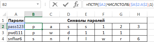
Получим массивы символов для каждого из паролей:

Функция ПСТР возвращает часть строки, ограниченную номерами позиций символов, указанных в качестве второго и третьего аргумента. Поскольку требуется вывести 1 символ, третий аргумент принимает значение 1. Функция ЧИСЛСТОЛБ($A$2:G$2) с зафиксированными ячейками (символ $) возвращает требуемый номер столбца, соответствующий номеру символа в строке.

Растянем данную формулу по строке и получим следующее:

Для получения шифра первого пароля используем следующую формулу массива:

Примечание:

Данная формула была записана в ячейку B7, поскольку формулы массивов не могут выполняться в объединенных ячейках. Аналогично сгенерируем шифры для остальных паролей:

Недостаток метода состоит в том, что для дешифрации (обратного преобразования) требуются ключи, указывающие на количество цифр, соответствующих числовому обозначению символа в Юникод.

Особенности кодирования с использованием функции UNICODE в Excel

Функция имеет следующую синтаксическую запись:

=UNICODE(текст)

Единственным аргументом, обязательным для заполнения, является текст – текстовая строка или один символ, для которого требуется определить соответствующее числовое значение кодировки Юникод.

Примечания:

1. Несмотря на то, что данная функция принимает на вход текстовую строку, фактически числовое представление определяется для первого символа строки. То есть, результаты выполнения функций =UNICODE(«слово») и =UNICODE(«с») будут эквивалентны, поскольку числовое представление определяется для символа «с» — 1089.
2. При работе с данными логического типа выполняется промежуточное преобразование к текстовым данным. Например, функции =UNICODE(ИСТИНА) и =UNICODE(«ИСТИНА») вернут одинаковое значение 1048, поскольку строчная «И» представлена числовым кодом 1048.
3. При вводе имен будет возвращен код ошибки #ИМЯ? (например, =UNICODE(табл1)).