
Excel для Microsoft 365 Excel для Microsoft 365 для Mac Excel для Интернета Excel 2021 Excel 2021 для Mac Excel 2019 Excel 2019 для Mac Excel 2016 Excel 2016 для Mac Excel 2013 Excel 2010 Excel 2007 Excel для Mac 2011 Excel Starter 2010 Еще…Меньше
В этой статье описаны синтаксис формулы и использование функции ПИ в Microsoft Excel.
Описание
Возвращает число 3,14159265358979 — математическую константу «пи» с точностью до 15 цифр.
Синтаксис
ПИ()
У функции ПИ нет аргументов.
Пример
Скопируйте образец данных из следующей таблицы и вставьте их в ячейку A1 нового листа Excel. Чтобы отобразить результаты формул, выделите их и нажмите клавишу F2, а затем — клавишу ВВОД. При необходимости измените ширину столбцов, чтобы видеть все данные.
|
Данные |
||
|
Радиус |
||
|
3 |
||
|
Формула |
Описание |
Результат |
|
=ПИ() |
Возвращает число «пи». |
3,141592654 |
|
=ПИ()/2 |
Возвращает число «пи», разделенное на 2. |
1,570796327 |
|
=ПИ()*(A3^2) |
Площадь круга с радиусом, указанным в ячейке A3. |
28,27433388 |
Нужна дополнительная помощь?
Для получения числа Пи нужно написать:
=ПИ()
Нажав клавишу ВВОД, мы получим результат 3,141592654.
У функции ПИ нет аргументов.
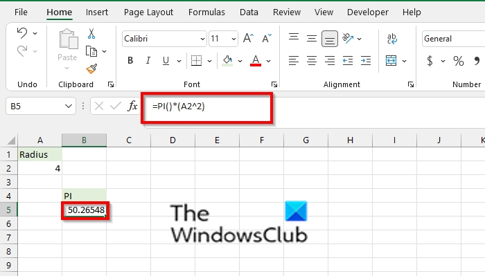
С помощью функции ПИ в Excel, зная радиус круга, можно вычислить его площадь.
Формула будет выглядеть так:
=ПИ()*(A2^2),
где A2 – это ячейка, в которую вписано значение радиуса.
Например, радиус круга равен 5. Записав формулу и нажав клавишу ВВОД, мы получим площадь круга, равную 78,53981634.
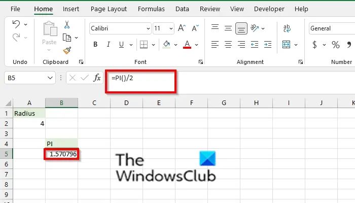
Еще одна функция, которая есть в Excel, возвращает половину числа Пи. Выглядит эта запись так:
=ПИ()/2
Нажав клавишу ВВОД, мы получим 1,570796327.
Число Пи — справочные материалы
Число Пи — значение, история, кто придумал
Как запомнить число Пи
Чему равно число Пи
Число Пи на клавиатуре и в Word
Фотографии числа Пи
Геометрические фигуры
Download PC Repair Tool to quickly find & fix Windows errors automatically
The PI function in Microsoft Excel is a Math and Trigonometry function, and it returns the value of PI. The formula for the PI formula is =PI (). The PI function syntax has no arguments.
Follow the steps below to use the PI function in Microsoft Excel:
- Launch Microsoft Excel
- Create a table or use an existing table from your files
- Place the formula into the cell you want to see the result
- Press the Enter Key
Launch Microsoft Excel.
Create a table or use an existing table from your files.

Place the formula =PI() into the cell you want to see the result.
Press the Enter key to see the result.
Excel will return the PI 3.141593.
Type into the cell =PI()/2 and press enter. Excel will return the PI divided by 2, which gives the result of 1.570796.
Type into the cell =PI()*(A2^2) and press enter. Excel will return the result 50.26548. The A2 cell contains the area of the circle with a radius.
There are two other methods to use the PI function.
Method one is to click the fx button on the top left of the Excel worksheet.
An Insert Function dialog box will appear.
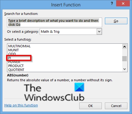
Inside the dialog box in the section, Select a Category, select Math and Trigonometry from the list box.
In the section Select a Function, choose the PI function from the list.
Then click OK.
A Function Arguments dialog box will open.
Then click OK.
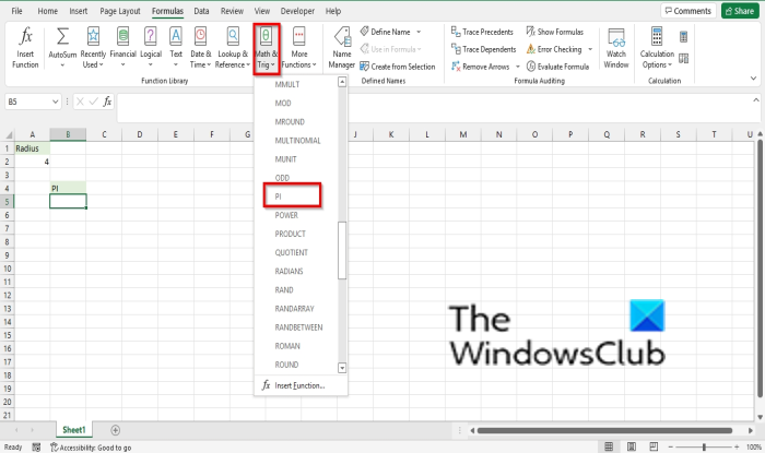
Method two is to click the Formulas tab, then click the Math and Trigonometry button in the Function Library group.
Then select PI from the drop-down menu.
A Function Arguments dialog box will open.
What does PI mean in math?
In Math, Pi is defined as the ratio of a circle’s circumference to its diameter. The value of PI is 3.14, and regardless of circle size, this ratio will always equal PI. PI is written as the Greek letter for p or π.
How to multiply by PI in Excel?
Excel is a program that can be used to calculate math. Normally, when users multiply PI in Excel, it is when they want to calculate the area of the circle from the diameter or radius; for example, calculating an area of the circle from the diameter, =PI()*3 or calculating an area of the circle from the radius =PI()/4*3^2.
We hope this tutorial helps you understand how to use the PI function in Microsoft Excel; if you have questions about the tutorial, let us know in the comments.
Shantel has studied Data Operations, Records Management, and Computer Information Systems. She is quite proficient in using Office software. Her goal is to become a Database Administrator or a System Administrator.
В этом учебном материале вы узнаете, как использовать Excel функцию ПИ с синтаксисом и примерами.
Описание
Microsoft Excel функция ПИ возвращает математическую константу, которая равна 3,14159265358979.
Функция ПИ — это встроенная в Excel функция, которая относится к категории математических / тригонометрических функций.
Её можно использовать как функцию рабочего листа (WS) в Excel.
В качестве функции рабочего листа функцию ПИ можно ввести как часть формулы в ячейку рабочего листа.
Синтаксис
Синтаксис функции ПИ в Microsoft Excel:
ПИ()
Аргументы или параметры
Для функции ПИ нет параметров или аргументов.
Возвращаемое значение
Функция ПИ возвращает число π, равное 3,14159265358979.
Применение
- Excel для Office 365, Excel 2019, Excel 2016, Excel 2013, Excel 2011 для Mac, Excel 2010, Excel 2007, Excel 2003, Excel XP, Excel 2000
Тип функции
- Функция рабочего листа (WS)
Пример (как функция рабочего листа)
Рассмотрим несколько примеров функции ПИ, чтобы понять, как использовать Excel функцию ПИ как функцию рабочего листа в Microsoft Excel:

Hа примере приведенной выше электронной таблицы Excel, будут возвращены следующие примеры функции ПИ:
|
=ПИ() Результат: 3.141592654 =ПИ() * A1 Результат: 47.1238898 =ПИ() / A2 Результат: 0.285599332 =ПИ() + A3 Результат: —5.858407346 |
Читайте также:
- как найти площадь круга.
- как найти длину окружности
Число Пи — математическая константа с приблизительным значением 3,1415926535897.
Числа Пи можно найти во многих тригонометрических и геометрических формулах. Особенно формулы, относящиеся к кругам, эллипсам и сферам:
- Длина окружности равна произведению числа Пи на диаметр.
- Площадь круга равна произведению числа Пи на квадрат радиуса.
Excel разработал функцию Пи, чтобы помочь пользователям применять тригонометрические формулы при использовании программного обеспечения. В этой статье советы по программному обеспечению помогут вам синтаксис и использование констант Pi в Excel.
Синтаксис функции: = PI ().
Функция Пи не имеет аргументов.
Пример 1. В ячейке A1 введите формулу = PI (), результат: 3,141593.
Пример 2: у вас есть диаметр круга в ячейке B2, и вам нужно вычислить длину окружности в ячейке B4 и площадь круга в этой ячейке B5. Вы применяете следующую геометрическую формулу:
В4 = ПИ () * 2 * В2,
B5 = PI () * B2 ^ 2.
И вы получите следующий результат:
Вышеупомянутое программное обеспечение Dexterity помогло вам прочитать синтаксис функции и узнать, как использовать функцию Pi в Excel. Удачи.
Число Пи очень часто используется в различных вычислениях, например, для расчета длины окружности, объема цилиндра или сферы.
Рассмотрим варианты использования числа Пи в Excel.
Для начала немного справочной информации.
Число Пи — отношение длины окружности к длине её диаметра, математическая константа приблизительно равная 3,14.
В Excel также можно использовать другую известную математическую константу — число Эйлера.
Что записать число Пи достаточно воспользоваться стандартной функцией:
ПИ()
Возвращает округленное до 15 знаков после запятой число Пи (значение 3,14159265358979).
Обратите внимание, что данная функция не имеет аргументов.

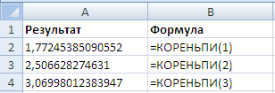
Функция КОРЕНЬПИ в Excel
Также в Excel есть функция, позволяющая вычислить квадратный корень из числа Пи:
КОРЕНЬПИ(число)
Возвращает квадратный корень из значения выражения (число * ПИ).
- Число (обязательный аргумент) — число, на которое умножается Пи.
Удачи вам и до скорой встречи на страницах блога Tutorexcel.ru!
Поделиться с друзьями:
Поиск по сайту:
Want to take your Excel skills to the next level? Learn how to use Excel’s PI function to simplify data analysis and perform complex calculations.
![]()
The pi number (π) is a mathematical constant defined as the circumference of a circle divided by its diameter. Although pi is roughly equal to 3.14, in some cases, you might need a more exact value for your calculations.
The good news is that Excel knows the pi number to its 15th digit by heart. You can summon Excel’s recitation of pi using the PI function, and even combine it with other Excel functions.
The PI Function in Excel: How Does It Work?
PI is a simple Excel function that returns the pi number with 14 decimals. It only does that and takes in no arguments.
=PI()
If used alone in a formula, PI simply returns the pi number. You can perform mathematical operations on the PI function, and use it in combination with other functions.
How to Use the PI Function in Excel
As the PI function in Excel doesn’t have any arguments, its usage consists of simply calling it in a formula. Here’s how you can display the pi number using PI:
- Select the cell where you want to display the pi number.
- In the formula bar, enter the formula below:
=PI() - Press Enter.
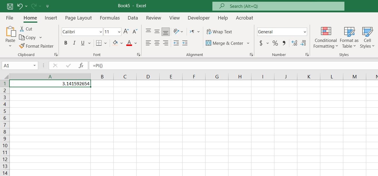
Excel will now display the pi number, accurate to 15 digits. If you don’t want to display all 15 digits, you can use custom formatting in Excel to limit the decimals.
Using PI for Calculations in Excel
Displaying the pi number isn’t all that there is to the PI function. Since PI takes in no arguments, Excel treats it more like a numerical value rather than a function.
This means that you can simply call PI in your formula, and then perform mathematical operations on it. Let’s see this in action with an example.
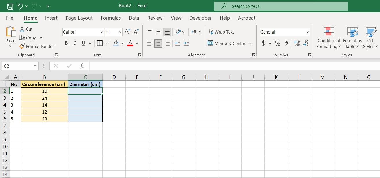
In this spreadsheet, we’ve got the circumference of five circles, and the goal is to calculate their diameters. Since a circle’s circumference is its diameter multiplied by pi, we can achieve this goal with a simple division.
- Select the first cell where you want to display the results. That will be cell C2 in this example.
- In the formula bar, enter the formula below:
=B2/PI() - Press Enter.
- Grab the fill handle and drop it on the cells below.
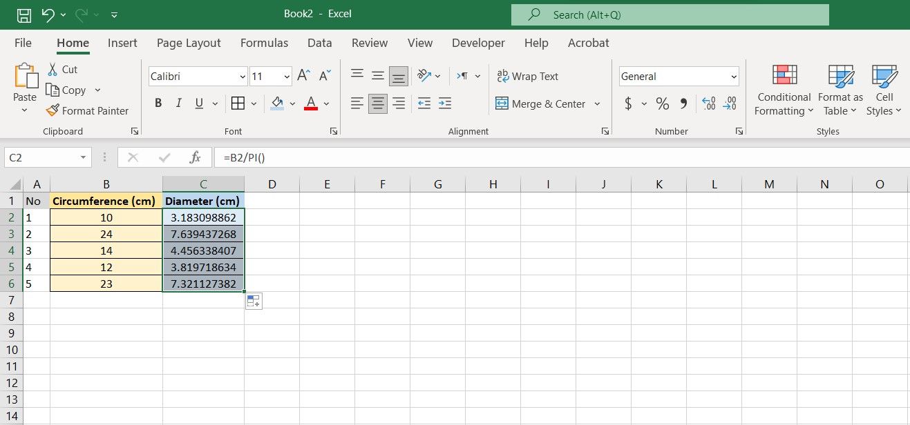
You should now see the diameter for each circle. The formula here takes the circumference value in cell B2 and then divides it by the pi number using the PI function.
Using PI With Other Excel Functions
You can also use PI in any Excel function that takes in numerical values. This comes in extra handy when you’re using trigonometric functions in Excel.
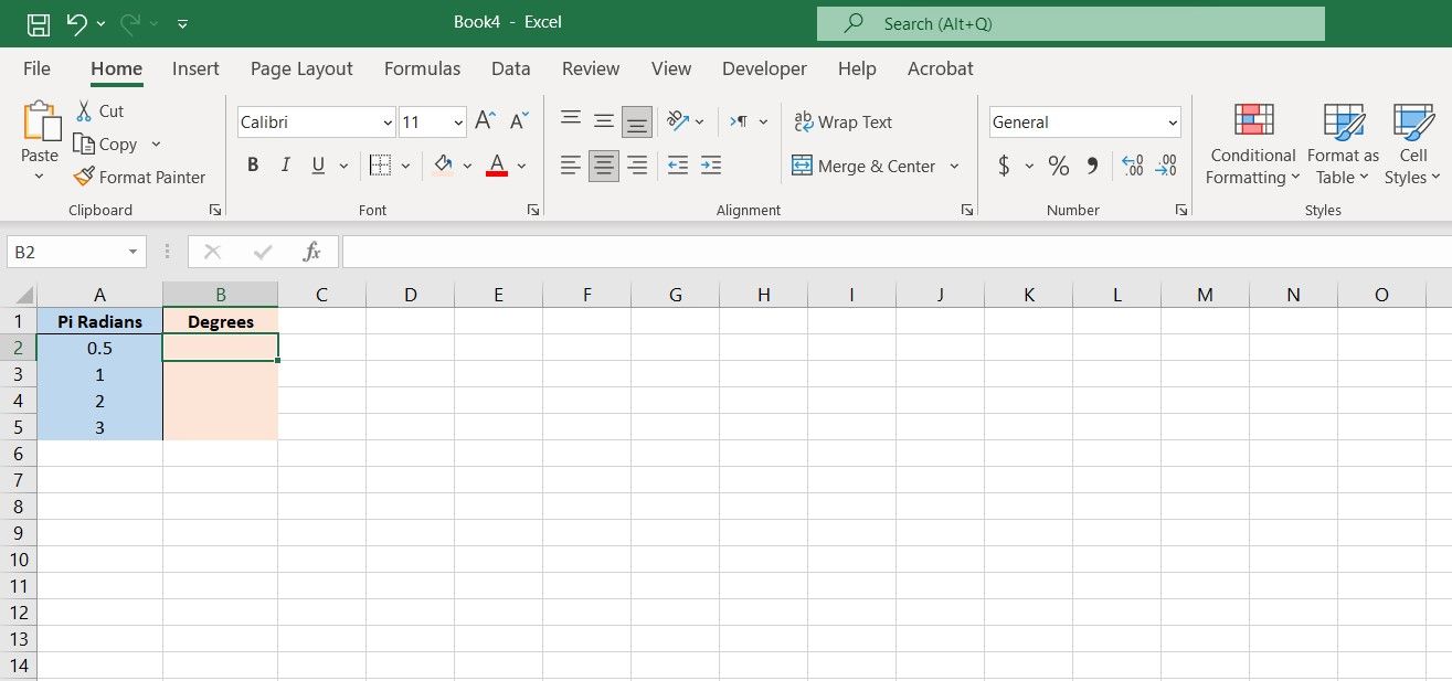
In this example, we have some angles in pi radians and want to convert them to the more feasible degrees. Pi radians is one radian multiplied by pi.
For this task, we’re going to use a combination of the PI function and the DEGREES function. DEGREES is an Excel function that takes in radian values, and converts them to degrees.
=DEGREES(value_in_radians)
Here’s how you can convert pi radians to degrees in Excel:
- Select the cell where you want to display the results.
- In the formula bar, enter the formula below:
=DEGREES(A2*PI()) - Press Enter.
- Drag the fill handle and drop it on the cells below.
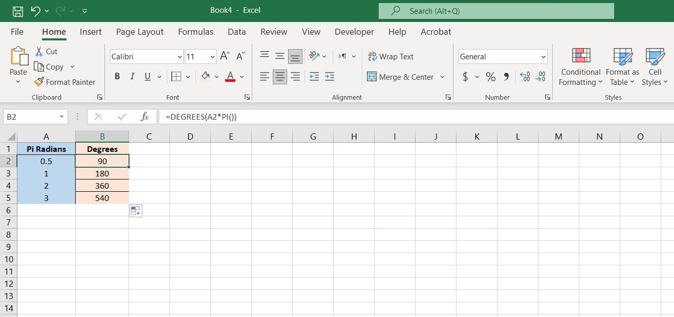
Now you’ll see the angles’ equivalent in degrees. The formula we used calls on the DEGREES function and feeds it the value in radians (A2) multiplied by the pi number. You can use the CONVERT function in Excel to convert other units.
Forget About Pi’s Actual Value
The pi number is one of the most important mathematical constants. As far as modern computing capabilities go, pi has an infinite number of decimals. The PI function in Excel returns the pi number up to its 15th digit.
This way, you don’t have to enter the pi number manually, and sure enough, you don’t have to try and memorize its digits for minute calculations. Excel’s PI function can be used in other functions, providing you with the pi number in any formula where you might need it.