
Если функция F(x) непрерывна на отрезке [a, b] и имеет внутри этого отрезка локаль-ный экстремум, то его можно найти, используя надстройку Excel Поиск решения. Рассмотрим последовательность нахождения экстремума функции на примере.
Пример 12. Задана неразрывная функция Y= X 2 +X +2. Требуется найти ее экстремум (минимальное значение) на отрезке [-2, 2].
Решение:
1. В ячейку А3 рабочего листа введите любое число, принадлежащее заданному отрезку, в этой ячейке будет находиться значение Х.
2. В ячейку В3 введите формулу, определяющую заданную функциональную зависимость (рис. 18). Вместо переменной Х в этой формуле должна быть ссылка на ячейку А3: = A2^2 + A2 +2.
3. Выполните команду меню Сервис — Поиск решения.
4. В открывшемся окне диалога Поиск решения в поле Установить целевую ячейку укажите адрес ячейки, содержащей формулу (В3), установите пере-ключатель Минимальному значению, в поле Изменяя значение ячейки укажите адрес ячейки, в которой содержится переменная х.
5. Добавьте два ограничения в соответствующее поле: A3>= -2 и A3<= 2.
6. Щелкните на кнопке Параметры и в от крывшемся диалоговом окне Пара-метры поиска решения установите относительную погрешность вычислений и предельное число итераций.
7. Щелкните на кнопке Выполнить.
В ячейке А3 будет помещено значение аргумента Х функции, при котором она принимает минимальное значение, а в ячейке В3 – минимальное значение функции. В результате выполнения вычислений в ячейке А3 будет получено значение независимой переменной, при котором функция принимает наименьшее значение, а в ячейке В3 – минимальное значение функции, равное 1,75. Постройте график заданной функции и убедитесь, что решение найдено верно.
Поиск решения MS EXCEL. Экстремум функции с несколькими переменными. Граничные условия заданы уравнениями
history 14 января 2021 г.
- Группы статей
- Надстройка «Поиск решения»
Пусть дана функция с несколькими переменными F(x1, x2, . )=a1*x1+a2*x2+. Также даны граничные условия в виде b1*x1+b2*x2+. файл примера ).

Переменные (выделено зеленым) . В качестве переменных модели, очевидно, выступают x1, x2, x3, x4. Эта задача хороша тем, что переменные задаются однозначно, не требуется осмысливать житейскую задачу, например как с оптимизацией затрат . Хотя математически — это эквивалентные задачи, только количество переменных разное.
После запуска Поиск решения будет методично (последовательно) по своему алгоритму подставлять в зеленые ячейки числовые значения и вычислять функцию F (красная ячейка).
Ограничения (выделено серым) . Ограничения модели — это ограничения на область изменения переменных. Они могут задаваться как простыми выражениями для одной переменной, например х1>=0, так и для некой комбинации переменных 5*x1+4*x2-x3-2*x4 =0 ограничения можно ввести прямо в окне Поиска решения (будет показано ниже), для более сложных зависимостей удобно подготовить вспомогательную таблицу (С26:Е29).
Составить модель, особенно первую, непросто. Может помочь такой подход: считать, что переменные (зеленые ячейки) уже содержат некие значения, пусть даже не оптимальные. Так легче составлять огграничения. В нашем случае ограниечение 5*x1+4*x2-x3-2*x4 можно записать с помощью формулы = СУММПРОИЗВ($D$19:$D$22;C26:C29) . В диапазоне D19:D22 содержатся коэффициенты 5; 4; -1; -2. Кроме того, если значения переменных заданы, то и значение целевой функции также автоматически рассчитано (тоже не оптимальное пока, до запуска Поиска решения).
Целевая функция (выделено красным) . Целевая функция — это то, что требуется оптимизировать, т.е. F. Формула для ее вычисления задана в явном виде — не нужно догадываться из условий обычной задачи как ее подсчитать. Это не всегда очевидно (см., например, статью про пропускную способность трубопровода ).
Ниже приведено окно Поиска решения с заполненными полями: целевая функция, переменные и ограничения.

После запуска Поиска решения ответ будет вычислен за доли секунды: F=3.
Section 6.3 Critical Points and Extrema
Subsection 6.3.1 Critical Points
With functions of one variable we were interested in places where the derivative is zero, since they made candidate points for the maximum or minimum of a function. If the derivative is not zero, we have a direction that is downhill and moving a little in that direction gives a lower value of the function. Similarly, with functions of two variables we can only find a minimum or maximum for a function if both partial derivatives are 0 at the same time. Such points are called critical points.
The point ((a,b)) is a critical point for the multivariable function (f(x,y)text{,}) if both partial derivatives are 0 at the same time.
In other words,
begin{equation*}
frac{partial }{partial x} f(x,y)|_{x=a,y=b}=0
end{equation*}
and
begin{equation*}
frac{partial }{partial y} f(x,y)|_{x=a,y=b}=0text{.}
end{equation*}
Example 6.3.1. Finding a Local Minimum of a Function.
Use the partial derivatives of (f(x,y)=x^2+ 2xy+3y^2-4x-3y) to find the minimum of the graph.
Solution.
- Critical Point by Algebra
-
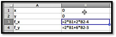
In the previous section, we already computed
begin{align*}
frac{partial }{partial x} f(x,y) amp = 2x+2y-4\
frac{partial }{partial y} f(x,y) amp = 2x+6y-3text{.}
end{align*}We need to find the places where both partial derivatives are 0. With this simple system, I can solve this system algebraically and find the only critical point is ((9/4, -1/4)text{.})
begin{align*}
0 amp = 2x+2y-4\
0 amp = 2x+6y-3text{.}
end{align*}Subtract the equations to eliminate (xtext{:})
begin{equation*}
0=0-4y-1text{.}
end{equation*}Solve for (ytext{:})
begin{align*}
4y amp = -1\
y amp = -1/4text{.}
end{align*}Substitute back and solve for (xtext{:})
begin{align*}
0 amp = 2x+2(-1/4)-4\
2x amp = 9/2\
x amp =9/4text{.}
end{align*} - Critical Point by Solver
-
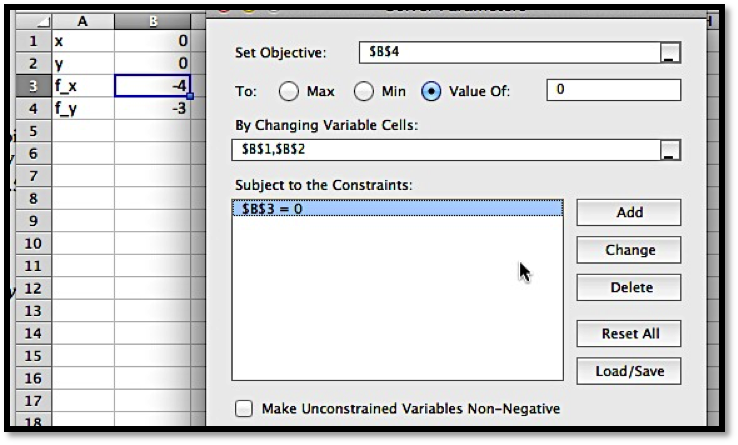
If the partials are more complicated, I will want to find the critical points another way. I can find the point with Solver.

To get solver to set both partials to 0 at the same time, I ask it to solve for (f_y=0text{,}) while setting (f_x=0) as a constraint. Make sure to uncheck the box that makes unconstrained variables non-negative.
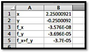
This finds our critical point within our error tolerance.
- Critical Point by CAS
-
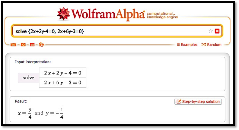
We can also use Wolfram|Alpha to find the solution to our system of equations.
- Determining the Critical Point is a Minimum
-
We thus get a critical point at ((9/4,-1/4)) with any of the three methods of solving for both partial derivatives being zero at the same time. Once we have a critical point we want to determine if it is a maximum, minimum, or something else. The easiest way is to look at the graph near the critical point.
It is clear from the graph that this critical point is a local minimum.
It is easy to see that (f(x,y)=x^2+y^2) has a critical point at ((0,0)) and that that point is a minimum for the function. Similarly, (f(x,y)=-x^2-y^2) has a critical point at ((0,0)) and that that point is a maximum for the function. For some functions, like (f(x,y)=x^2-y^2text{,}) which has a critical point at ((0,0)text{,}) we can have a maximum in one direction and a minimum in another direction. Such a point is called a saddle point. We note that we can have a saddle point even if the (x) and (y) slice curves both indicate a minimum.
Example 6.3.3. A Saddle Point at a Minimum on Both Axes.
Show that (f(x,y)=x^2-3xy+y^2) has a critical point at ((0,0)text{,}) which is a minimum of both slice curves, but is not a local minimum.
Solution.
We look at the two partial derivatives, and notice they are both zero at the origin.
begin{align*}
frac{partial }{partial x} f(x,y) amp = 2x-3y\
frac{partial }{partial x} f(x,y) amp = -3x+2ytext{.}
end{align*}
We then see that both slice curves are parabolas that bend up, with a minimum at 0.
begin{align*}
f(x,0) amp = x^2\
f(0,y) amp = y^2text{.}
end{align*}
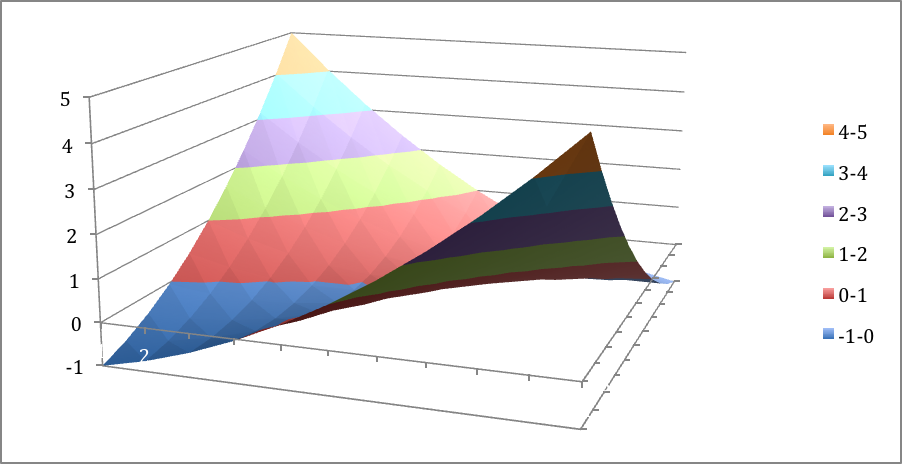
However if we take the slice with (x=ytext{,}) we get a parabola bending down, so we don’t have a minimum.
begin{equation*}
f(x,-x)=x^2-3x x+x^2=-x^2text{.}
end{equation*}
Looking at the graph, we see that this graph does not have a minimum.
Subsection 6.3.2 Second Partial Derivatives
With only first derivatives, we can just find the critical points. To check if a critical point is maximum, a minimum, or a saddle point, using only the first derivative, the best method is to look at a graph to determine the kind of critical point. For some applications we want to categorize the critical points symbolically.
With functions of one variable we used the second derivative to test if a critical point was a maximum or minimum. In the two variable case we need to define the second derivatives and use them to define the discriminant of a function to test if a critical point is a minimum, maximum, or saddle point. We first need to define second partial derivatives.
Second partials.
begin{equation*}
f_{ab}=(f_a )_b=frac{partial}{partial b}(frac{partial}{partial a} f)text{.}
end{equation*}
Note that (f_{xx}) is simply the old second derivative of the curve (f(x,y_0)) and (f_{yy}) is simply the old second derivative of the curve (f(x_0,y)text{.}) For functions with continuous second partial derivatives, the mixed partials, (f_{yx}) and (f_{xy}) are the same.
Example 6.3.5. Finding Second Partial Derivatives.
Find the second partial derivatives of
begin{equation*}
f(x,y)=x^2+ 3xy+5y^3-7x-11ytext{.}
end{equation*}
Solution.
We start by computing the first partial derivatives.
begin{align*}
f_x amp = frac{partial}{partial x} f(x,y)=2x+3y-7\
f_y amp = frac{partial}{partial y} f(x,y)=3x+15y^2-11text{.}
end{align*}
Then we compute the second partial derivatives.
begin{align*}
f_{xx} amp = frac{partial}{partial x} f_x=2\
f_{xy} amp = frac{partial}{partial y} f_x=3\
f_{yx} amp = frac{partial}{partial x} f_y=3\
f_{yy} amp = frac{partial}{partial y} f_y=30ytext{.}
end{align*}
As expected, the mixed partials are the same.
Subsection 6.3.3 Using the Discriminant to Test Critical Points
To test if a critical point is a maximum, minimum, or saddle point we compute the discriminant of the function.
Discriminant.
begin{equation*}
D(f(x,y))=f_{xx} f_{yy}-f_{xy}^2text{.}
end{equation*}
Example 6.3.6. Finding the Discriminant of a Function.
Find the discriminant of
begin{equation*}
f(x,y)=x^2+ 3xy+5y^3-7x-11ytext{.}
end{equation*}
Solution.
We have already computed the second partial derivatives.
begin{equation*}
f_xx=2,quad f_xy=3,quad f_yy=30ytext{.}
end{equation*}
Substituting into the formula,
begin{equation*}
D=(2)(30y)-3^2=60y-9text{.}
end{equation*}
Discriminant test.
Let ((a,b)) be a critical point of (f(x,y)text{.})
If (D(a,b)>0) and (f_{xx} (a,b)>0) then ((a,b)) is a local minimum of (f(x,y)text{.})
If (D(a,b)>0 ) and (f_{xx} (a,b)lt 0) then ((a,b)) is a local maximum of (f(x,y)text{.})
If (D(a,b)lt 0) then ((a,b)) is a saddle point of (f(x,y)text{.})
If (D(a,b)=0) we do not have enough information to classify the point.
Example 6.3.7. Using the Discriminant to Classify Critical Points.
Based on the information given, classify each of the following points as a local maximum, local minimum, saddle point, not a critical point, or not enough information to classify.
| p | ({f_x}) | ({f_y}) | (f_{xx}) | (f_{xy}) | (f_{yy}) |
| A | 0 | 0 | 0 | 0 | 1 |
| B | 0 | 1 | 3 | 2 | 4 |
| C | 1 | 0 | 0 | 2 | 3 |
| D | 0 | 0 | 1 | 2 | 0 |
| E | 0 | 0 | -1 | 2 | 3 |
| F | 0 | 0 | -3 | 1 | -2 |
| G | 0 | 0 | 3 | 3 | 3 |
Solution.
We need to compute the discriminant and apply the test.
| p | (f_x) | (f_y) | (f_{xx}) | (f_{xy}) | (f_{yy}) | Discriminant | Classification |
| A | 0 | 0 | 0 | 0 | 1 | 0 | Not enough information |
| B | 0 | 1 | 3 | 2 | 4 | 8 | Not a critical point |
| C | 1 | 0 | 0 | 2 | 3 | -4 | Not a critical point |
| D | 0 | 0 | 1 | 2 | 0 | -4 | Saddle point |
| E | 0 | 0 | -1 | 2 | 3 | -7 | Saddle point |
| F | 0 | 0 | -3 | 1 | -2 | 5 | Maximum |
| G | 0 | 0 | 3 | 3 | 3 | 0 | Not enough information |
Example 6.3.8. Finding and Classifying Critical Points.
Let (f(x,y)=x^3-3x+y^3-3y^2text{.}) Find the critical points and classify them using the discriminant.
Solution.
We start by computing the first partial derivatives.
begin{align*}
f_x amp = 3x^2-3=3(x-1)(x+1)\
f_y amp = 3y^2-6y=3(y-2)(y)text{.}
end{align*}
Then we compute the second partial derivatives and the discriminant.
begin{equation*}
f_{xx}=6x,quad f_{xy}=0,quad f_{yy}=6y-6,quad D=(6x)(6y-6)-0^2=36xy-36xtext{.}
end{equation*}
We have critical points when both first partials are 0, so at ((1,2)text{,}) ((-1,2)text{,}) ((1,0)text{,}) and ((-1,0)text{.})
At ((1,2)text{,}) both (D) and (f_{xx}) are positive, so we have a local minimum.
At ((-1,2)) and ((1,0)text{,}) (D) is negative, so we have a saddle point.
At (((-1,0)text{,}) (D) is positive and (f_{xx}) is negative, so we have a local maximum.
Exercises 6.3.4 Exercises: Critical Points and Extrema Problems
Exercise Group.
For the given functions and region:
-
Find the partial derivatives of the original function.
-
Find any critical points in the region.
-
Produce a small graph around any critical point.
-
Determine if the critical points are maxima, minima, or saddle points.
1.
The function is (f(x,y)=x^2+2xy+4y^2+5x-6ytext{,}) for the region (-10le xle 10text{,}) and (-10le yle 10text{.})
Solution.
-
begin{align*}
f_x (x,y) amp = 2x+2y+5\
f_y (x,y) amp = 2x+8y-6text{.}
end{align*} -
Set the partial derivatives equal to 0 and solve for (x) and (ytext{.})
begin{align*}
f_x (x,y) amp = 2x+2y+5=0\
f_y (x,y) amp = 2x+8y-6=0text{.}
end{align*}We can use either the method of substitution (solve for (x) or (y) in one equation and substitute into the other and solve), or method by elimination (multiply both equations by carefully chosen numbers and ass/subtract the equations from each other.)
We will demonstrate method of elimination:
begin{align*}
-1×(2x+2y+5 amp = 0) amp text{gives }-2x-2y-5amp=0\
1×(2x+8y-6 amp = 0) amp text{gives } 2x+8y-6amp =0text{.}
end{align*}Adding the two equations gives (6y-11=0text{;}) hence, (y= 11/6text{.})
Pick one of the equations to solve for x (it does not matter which one):
begin{equation*}
2x+2y+5=0 quad text{and }y= 11/6
end{equation*}implies that (2x+2(11/6)+5=0) so (x= (2(11/6)+5)/(-2)=-13/3text{.})
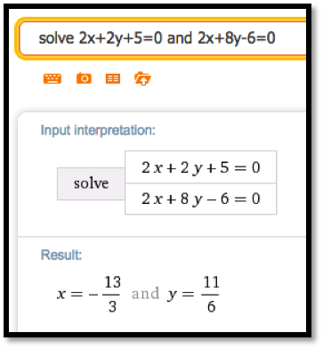
We can also solve this system of equations using Wolfram Alpha:
-
The command in Wolfram Alpha is:
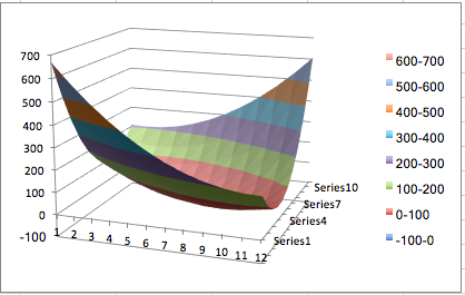
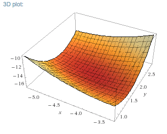
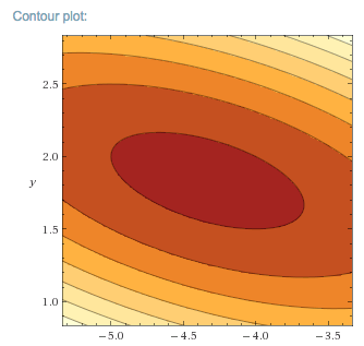
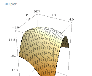
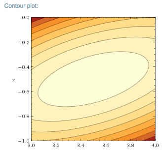
It is worth looking at both the 3D Plot and the Contour Plot.
-
The 3D plot suggests a minimum, and this is confirmed by the contour plot which shows they typical view of a local minimum.
As an alternative we can find the discriminant.
begin{align*}
f_{xx} (x,y) amp = 2\
f_{xy} (x,y) amp = 2\
f_{yy} (x,y) amp = 8\
D amp = f_{xx} (x,y)f_{yy} (x,y)-f_{xy} (x,y)^2=2*8-2^2=12>0text{.}
end{align*}Since (Dgt 0) and (f_{xx} (x,y)gt 0) we have a local minimum.

2.
The function is (f(x,y)=x^2+7xy+2y^2+4x-3ytext{,}) for the region (-10le xle 10text{,}) and (-10le yle 10text{.})
3.
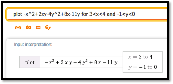
The function is (f(x,y)=-x^2+2xy-4y^2+8x-11ytext{,}) for the region (-10le xle 10text{,}) and (-10le yle 10text{.})
Solution.
-
begin{align*}
f_x (x,y) amp = -2x+2y+8\
f_y (x,y) amp = 2x-8y-11text{.}
end{align*} -
Set the partial derivatives equal to 0 and solve for (x) and (ytext{.})
begin{align*}
f_x (x,y) amp = -2x+2y+8=0\
f_y (x,y) amp = 2x-8y-11=0text{.}
end{align*}Adding the equations (-6y-3=0text{,}) and so (y=-1/2text{.})
Substituting in the first equation give (-2x+7=0text{,}) and so (x=7/2text{.})
Hence we have a critical points at ((7/2,-1/2)text{.})
-
For ((x,y)= (2,1)text{:})
-
From the picture we conclude that the critical point is a maximum. As an alternative we can find the discriminant.
begin{align*}
f_{xx} (x,y) amp = -2\
f_{xy} (x,y) amp = 2\
f_{yy} (x,y) amp = -8\
D amp = f_{xx} (x,y)f_{yy} (x,y)-f_{xy} (x,y)^2=2*8-2^2=12gt 0text{.}
end{align*}Since (Dgt 0) and (f_{xx} (x,y)lt 0) we have a local maximum.
4.
The function is (f(x,y)=x^3-12x+y^3-3ytext{,}) for the region (-10le xle 10text{,}) and (-10le yle 10text{.})
5.
The function is the revenue function for selling widgets and gizmos with demand price functions
begin{align*}
PriceGizmo amp = 25-frac{QuantityGizmo}{50}-frac{QuantityWidget}{200}\
PriceWidget amp = 30-frac{QuantityWidget}{45}-frac{QuantityGizmo}{300}
end{align*}
for the region (0le QuantityWidgetle 1500text{,}) and (0le QuantityGizmole 1500text{.})
Solution.
To solve this problem we will rename Gizmos (x) and Widgets (ytext{.}) This will make using Wolfram Alpha slightly easier, and symbol manipulation a tad more straight forward.
begin{align*}
PriceX amp = 25-frac{x}{50}-frac{y}{200}\
PriceY amp = 30-frac{y}{45}-frac{x}{300}\
revenue (x,y) amp =x*PriceX+y *PriceY\
amp =x left[25-frac{x}{50}-frac{y}{200}right]+yleft[30-frac{y}{45}-frac{x}{300}right]\
amp = frac{-36x^2-15xy+45000x-40y^2+54000y}{1800} text{.}
end{align*}
-
begin{align*}
revenue_x (x,y)amp = frac{-24x-5y+1000}{600} \
revenue_y (x,y)amp = frac{-3x-16y+10800}{360}
end{align*} -
Using WolframALpha, the critical point is at ((62000/123, 23800/41) approx (504, 580.5)text{.})
-
Using WolframAlpha we get:
-
From the picture we conclude that the critical point is a maximum.
As an alternative we can find the discriminant.
begin{align*}
f_{xx} (x,y) amp = -frac{1}{25}\
f_{xy} (x,y) amp = -frac{1}{120}\
f_{yy} (x,y) amp = -frac{4}{25}\
D amp = f_{xx} (x,y)f_{yy} (x,y)-f_{xy} (x,y)^2 gt 0text{.}
end{align*}Since (Dgt 0) and (f_{xx} (x,y)lt 0) we have a local maximum.


6.
The function is the revenue function for selling widgets and gizmos with demand price functions
begin{align*}
PriceGizmo amp = 30(0.9)^{(QuantityGizmo/150) }-frac{QuantityWidget}{250}\
PriceWidget amp = 20(0.97)^{(QuantityWidget/50) }-frac{QuantityGizmo}{350}
end{align*}
for the region (0le QuantityWidgetle 1500text{,}) and (0le QuantityGizmole 1500text{.}) (Warning: There are several critical points.)
7.
Based on the information given, classify each of the following points as a local maximum, local minimum, saddle point, not a critical point, or not enough information to classify.
| p | (f_x) | (f_y) | (f_{xx}) | (f_{xy}) | (f_{yy}) |
| A | 1 | 2 | 3 | 4 | 5 |
| B | 0 | 0 | 0 | 0 | 0 |
| C | 0 | 1 | 2 | 5 | 3 |
| D | 0 | 0 | 2 | 2 | 2 |
| E | 0 | 0 | 1 | 2 | 3 |
| F | 0 | 0 | 0 | 1 | 0 |
| G | 0 | 0 | 0 | -1 | 0 |
Solution.
Add a column for D and classify.
| p | (f_x) | (f_y) | (f_{xx}) | (f_{xy}) | (f_{yy}) | (D) | Classification |
| A | 1 | 2 | 3 | 4 | 5 | -1 | Not Critical |
| B | 0 | 0 | 0 | 0 | 0 | 0 | Not Enough Info |
| C | 0 | 1 | 2 | 5 | 3 | -19 | Not Critical |
| D | 0 | 0 | 2 | 2 | 2 | 0 | Not Enough Info |
| E | 0 | 0 | 1 | 2 | 3 | -1 | Saddle Point |
| F | 0 | 0 | 0 | 1 | 0 | 0 | Not Enough Info |
| G | 0 | 0 | 0 | -1 | 0 | 0 | Not Enough Info |
8.
Based on the information given, classify each of the following points as a local maximum, local minimum, saddle point, not a critical point, or not enough information to classify.
| p | (f_x) | (f_y) | (f_{xx}) | (f_{xy}) | (f_{yy}) |
| A | 1 | 2 | 3 | 4 | 5 |
| B | 0 | 0 | 0 | 0 | 0 |
| C | 0 | 1 | 2 | 5 | 3 |
| D | 0 | 0 | 2 | 2 | 2 |
| E | 0 | 0 | 1 | 2 | 3 |
| F | 0 | 0 | 0 | 1 | 0 |
| G | 0 | 0 | 0 | -1 | 0 |
9.
Using polynomials of the form (f(x,y)=ax^3+bx^4+cy^3+dy^4text{,}) produce a function that has a critical point at ((0, 0)text{,}) of each type.
-
A local maximum.
-
A local minimum.
-
A saddle point where the function f(x,0) has a local maximum and f(0,y) has a local minimum.
-
A saddle point where the function f(x,0) and f(0,y) both have inflection points.
Solution.
It helps to consider the question with only one variable.
(f(x)=ax^3) has an inflection point at (x=0) and neither a max nor a minimum.
(f(x)=ax^4) has minimum at (x=0) if (agt 0) and a maximum if (alt 0text{.})
Since all terms are of degree at least three, all second partial derivatives are zero at the origin, so the discriminant test fails.
-
A local maximum: ((x,y) = -x^4-y^4text{.}) Both (x^4) and (y^4) are nonnegative, so the function is negative everywhere except at the origin where it is 0.
-
A local minimum: (f(x,y)= x^4+y^4text{.}) Both (x^4) and (y^4) are nonnegative, so the function is positive everywhere except at the origin where it is 0.
-
A saddle point where the function (f(x,0)) has a local maximum and (f(0,y)) has a local minimum: ((x,y)= -x^4+y^4text{.})
-
A saddle point where the function (f(x,0)) and (f(0,y)) both have inflection points: (f(x,y)= x^3+y^3)
You have attempted of activities on this page.
external/Examples/Section-6-3-Examples.xlsx
>>еще не может быть тем экстреммумом, который удовлетворяет моим условиям
Каким условиям? По вашему первому посту это понять не возможно.
Мне необходимо подстраиваться под вас и каждый раз добиваться внятных ответов? Потому что я пришёл на форум с просьбой ПОМОЧЬ в решении?
Почему тогда есть экстремум в 4 строке? Разница с 1 значением -1041, то есть, если
>>все значения правее- не превышают значений (А339+2000).
для этого случая нет значения (A4 — 2000) слева.
Честно говоря, вы меня утомили. Даю алгоритм поиска экстремума (через код в макросе) в общем виде следующий, дальше уже самостоятельно.
1. Определяем текущую точку в массиве на локальный экстремум, пусть значение в этой точке Хо. Формула выше есть для получения знака экстремума.
2. Если положительный экстремум.
2.1 Проверяем последовательно от точки экстремума, что точки слева/справа меньше Хо.
2.2 Критерий остановки проверки, что есть точки слева/справа такие, что (Xo-Xi)>=2000.
2.3 Если условия 2.1 и 2.2 выполнены, то считаем текущую точку — требуемым экстремумом и запоминаем индекс правой точки -1 для построения +1 в столбце 2
3. Аналогично, если в текущей точке отрицательный экстремум
3.1 слева/справа значения в точках больше
3.2 критерий остановки (Xi-Xo)>=2000
3.3 при выполнении условий 3.1 и 3.2 — отрицательный экстремум и запоминаем индекс правой точки — 1 для построения -1 в столбце 2