
Операторы слияния таблиц SQL JOIN в Excel | Power Query
Смотрите видео к статье:
Или операторы объединения таблиц SQL JOIN в Excel Power Query (начиная с Excel 2016)
Как известно самым популярным и эффективным инструментом работы с табличными данными (или просто таблицами) является программа Microsoft Excel.
При этом также известно, что самым мощным и распространённым языком программирования для работы с табличными данными является язык Structured Query Language = SQL = Язык структурированных запросов
Исходя из этого факта, логично предположить, что Microsoft Excel должен поддерживать язык SQL по умолчанию. Но, как правило, SQL поддерживается только базами данных (СУБД).
Несмотря на это, для Excel (начиная с 2010 версии) появилась бесплатная надстройка Power Query, которая позволяет имитировать часть полезного функционала языка SQL, а именно:
В языке SQL есть очень интересный оператор «SELECT», который позволяет делать запросы к табличным данным в базе данных. В результате запроса возвращается набор данных (выборка из базы данных), удовлетворяющий заданному условию выборки.
Как правило, выборка данных делается из нескольких таблиц в базе данных. Для связи таблиц в языке программирования SQL существует оператор «JOIN», который выполняет различные операции соединения реляционных таблиц (в основе этого принципа лежат законы реляционной алгебры)
Различают следующие виды оператора «JOIN»:
- INNER JOIN — Оператор внутреннего соединения двух таблиц
- LEFT OUTER JOIN — Оператор левого внешнего соединения двух таблиц
- RIGHT OUTER JOIN — Оператор правого внешнего соединения двух таблиц
- FULL OUTER JOIN — Оператор полного внешнего соединения двух таблиц
- CROSS JOIN — Оператор перекрёстного соединения (декартово произведение) двух таблиц
С выходом надстройки Power Query для Excel (это один из инструментов уровня Self-Service BI) в Excel появилась поддержка функционала всех видов операторов «JOIN» языка SQL:

Рассмотрим операторов «JOIN» в Excel на примерах:
Представим, что у нас в Excel есть две Таблицы: A «Люди» и B «Города»

Теперь давайте объединим данные таблицы с помощью различных операторов «JOIN»:
(объединяем таблицы через столбцы: A.Cityid = B.id)
Оператор INNER JOIN вернет следующий результат:

Оператор LEFT JOIN вернет следующий результат:

Оператор RIGHT JOIN вернет следующий результат:

Оператор FULL OUTER JOIN вернет следующий результат:

Оператор CROSS JOIN вернет следующий результат:

В надстройке Power Query для Excel данная функция «JOIN» называется «Слияние» — слияние запросов, где:
Оператору слияния INNER JOIN соответствует тип соединения: Внутреннее (только совпадающие строки)

Оператору слияния LEFT JOIN соответствует тип соединения: Внешнее соединение слева (все из первой таблицы, совпадающие из второй)

Оператору слияния RIGHT JOIN соответствует тип соединения: Внешнее соединение справа (все из второй таблицы, совпадающие из первой)

Оператору слияния FULL OUTER JOIN соответствует тип соединения: Полное внешнее (все строки из обеих таблиц)

Оператора слияния CROSS JOIN в интерфейсе Power Query нет, но его можно создать из оператора слияния FULL OUTER JOIN, убрав связи таблиц

Скачать Excel файл с примерами объединения SQL JOIN (функция «Слияние» в Power Query) можно скачать здесь
Пошаговая инструкция использования функции «Слияние»/«Объединения» в Power Query находится в видеоуроке к данной статье
Have you ever used VLOOKUP to bring a column from one table into another table? Now that Excel has a built-in Data Model, VLOOKUP is obsolete. You can create a relationship between two tables of data, based on matching data in each table. Then you can create Power View sheets and build PivotTables and other reports with fields from each table, even when the tables are from different sources. For example, if you have customer sales data, you might want to import and relate time intelligence data to analyze sales patterns by year and month.
All the tables in a workbook are listed in the PivotTable and Power View Fields lists.

When you import related tables from a relational database, Excel can often create those relationships in the Data Model it’s building behind the scenes. For all other cases, you’ll need to create relationships manually.
-
Make sure the workbook contains at least two tables, and that each table has a column that can be mapped to a column in another table.
-
Do one of the following: Format the data as a table, or Import external data as a table in a new worksheet.
-
Give each table a meaningful name: In Table Tools, click Design > Table Name > enter a name.
-
Verify the column in one of the tables has unique data values with no duplicates. Excel can only create the relationship if one column contains unique values.
For example, to relate customer sales with time intelligence, both tables must include dates in the same format (for example, 1/1/2012), and at least one table (time intelligence) lists each date just once within the column.
-
Click Data > Relationships.
If Relationships is grayed out, your workbook contains only one table.
-
In the Manage Relationships box, click New.
-
In the Create Relationship box, click the arrow for Table, and select a table from the list. In a one-to-many relationship, this table should be on the many side. Using our customer and time intelligence example, you would choose the customer sales table first, because many sales are likely to occur on any given day.
-
For Column (Foreign), select the column that contains the data that is related to Related Column (Primary). For example, if you had a date column in both tables, you would choose that column now.
-
For Related Table, select a table that has at least one column of data that is related to the table you just selected for Table.
-
For Related Column (Primary), select a column that has unique values that match the values in the column you selected for Column.
-
Click OK.
More about relationships between tables in Excel
-
Notes about relationships
-
Example: Relating time intelligence data to airline flight data
-
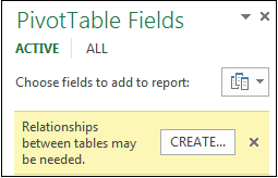
“Relationships between tables may be needed”
-
Step 1: Determine which tables to specify in the relationship
-
Step 2: Find columns that can be used to create a path from one table to the next
-
Notes about relationships
-
You’ll know whether a relationship exists when you drag fields from different tables onto the PivotTable Fields list. If you aren’t prompted to create a relationship, Excel already has the relationship information it needs to relate the data.
-
Creating relationships is similar to using VLOOKUPs: you need columns containing matching data so that Excel can cross-reference rows in one table with those of another table. In the time intelligence example, the Customer table would need to have date values that also exist in a time intelligence table.
-
In a data model, table relationships can be one-to-one (each passenger has one boarding pass) or one-to-many (each flight has many passengers), but not many-to-many. Many-to-many relationships result in circular dependency errors, such as “A circular dependency was detected.” This error will occur if you make a direct connection between two tables that are many-to-many, or indirect connections (a chain of table relationships that are one-to-many within each relationship, but many-to-many when viewed end to end. Read more about Relationships between tables in a Data Model.
-
The data types in the two columns must be compatible. See Data types in Excel Data Models for details.
-
Other ways to create relationships might be more intuitive, especially if you are not sure which columns to use. See Create a relationship in Diagram View in Power Pivot.
Example: Relating time intelligence data to airline flight data
You can learn about both table relationships and time intelligence using free data on the Microsoft Azure Marketplace. Some of these datasets are very large, requiring a fast internet connection to complete the data download in a reasonable period of time.
-
Start Power Pivot in Microsoft Excel add-in and open the Power Pivot window.
-
Click Get External Data > From Data Service > From Microsoft Azure Marketplace. The Microsoft Azure Marketplace home page opens in the Table Import Wizard.
-
Under Price, click Free.
-
Under Category, click Science & Statistics.
-
Find DateStream and click Subscribe.
-
Enter your Microsoft account and click Sign in. A preview of the data should appear in the window.
-
Scroll to the bottom and click Select Query.
-
Click Next.
-
Choose BasicCalendarUS and then click Finish to import the data. Over a fast internet connection, import should take about a minute. When finished, you should see a status report of 73,414 rows transferred. Click Close.
-
Click Get External Data > From Data Service > From Microsoft Azure Marketplace to import a second dataset.
-
Under Type, click Data.
-
Under Price, click Free.
-
Find US Air Carrier Flight Delays and click Select.
-
Scroll to the bottom and click Select Query.
-
Click Next.
-
Click Finish to import the data. Over a fast internet connection, this can take 15 minutes to import. When finished, you should see a status report of 2,427,284 rows transferred. Click Close. You should now have two tables in the data model. To relate them, we’ll need compatible columns in each table.
-
Notice that the DateKey in BasicCalendarUS is in the format 1/1/2012 12:00:00 AM. The On_Time_Performance table also has a datetime column, FlightDate, whose values are specified in the same format: 1/1/2012 12:00:00 AM. The two columns contain matching data, of the same data type, and at least one of the columns (DateKey) contains only unique values. In the next several steps, you’ll use these columns to relate the tables.
-
In the Power Pivot window, click PivotTable to create a PivotTable in a new or existing worksheet.
-
In the Field List, expand On_Time_Performance and click ArrDelayMinutes to add it to the Values area. In the PivotTable, you should see the total amount of time flights were delayed, as measured in minutes.
-
Expand BasicCalendarUS and click MonthInCalendar to add it to the Rows area.
-
Notice that the PivotTable now lists months, but the sum total of minutes is the same for every month. Repeating, identical values indicate a relationship is needed.
-
In the Field List, in “Relationships between tables may be needed”, click Create.
-
In Related Table, select On_Time_Performance and in Related Column (Primary) choose FlightDate.
-
In Table, select BasicCalendarUS and in Column (Foreign) choose DateKey. Click OK to create the relationship.
-
Notice that the sum of minutes delayed now varies for each month.
-
In BasicCalendarUS and drag YearKey to the Rows area, above MonthInCalendar.
You can now slice arrival delays by year and month, or other values in the calendar.
Tips: By default, months are listed in alphabetical order. Using the Power Pivot add-in, you can change the sort so that months appear in chronological order.
-
Make sure that the BasicCalendarUS table is open in the Power Pivot window.
-
On the Home table, click Sort by Column.
-
In Sort, choose MonthInCalendar
-
In By, choose MonthOfYear.
The PivotTable now sorts each month-year combination (October 2011, November 2011) by the month number within a year (10, 11). Changing the sort order is easy because the DateStream feed provides all of the necessary columns to make this scenario work. If you’re using a different time intelligence table, your step will be different.
“Relationships between tables may be needed”
As you add fields to a PivotTable, you’ll be informed if a table relationship is required to make sense of the fields you selected in the PivotTable.
Although Excel can tell you when a relationship is needed, it can’t tell you which tables and columns to use, or whether a table relationship is even possible. Try following these steps to get the answers you need.
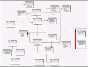
Step 1: Determine which tables to specify in the relationship
If your model contains just a few tables, it might be immediately obvious which ones you need to use. But for larger models, you could probably use some help. One approach is to use Diagram View in the Power Pivot add-in. Diagram View provides a visual representation of all the tables in the Data Model. Using Diagram View, you can quickly determine which tables are separate from the rest of the model.
Note: It’s possible to create ambiguous relationships that are invalid when used in a PivotTable or Power View report. Suppose all of your tables are related in some way to other tables in the model, but when you try to combine fields from different tables, you get the “Relationships between tables may be needed” message. The most likely cause is that you’ve run into a many-to-many relationship. If you follow the chain of table relationships that connect to the tables you want to use, you will probably discover that you have two or more one-to-many table relationships. There is no easy workaround that works for every situation, but you might try creating calculated columns to consolidate the columns you want to use into one table.
Step 2: Find columns that can be used to create a path from one table to the next
After you’ve identified which table is disconnected from the rest of the model, review its columns to determine whether another column, elsewhere in the model, contains matching values.
For example, suppose you have a model that contains product sales by territory, and that you subsequently import demographic data to find out if there is correlation between sales and demographic trends in each territory. Because the demographic data comes from a different data source, its tables are initially isolated from the rest of the model. To integrate the demographic data with the rest of your model, you’ll need to find a column in one of the demographic tables that corresponds to one you’re already using. For example if the demographic data is organized by region, and your sales data specifies which region the sale occurred, you could relate the two datasets by finding a common column, such as a State, Zip code, or Region, to provide the lookup.
Besides matching values, there are a few additional requirements for creating a relationship:
-
Data values in the lookup column must be unique. In other words, the column can’t contain duplicates. In a Data Model, nulls and empty strings are equivalent to a blank, which is a distinct data value. This means that you can’t have multiple nulls in the lookup column.
-
Data types of both the source column and lookup column must be compatible. For more information about data types, see Data types in Data Models.
To learn more about table relationships, see Relationships between tables in a Data Model.
Top of Page
If you work with Microsoft Excel, you may have to merge two files. In fact, that is a common task with Excel: consolidate information in a single item. However, doing that can be daunting with native Excel functions. In this post, we see how we can join tables in Excel in a way that mimics the SQL join statement.
To join tables in Excel, we are going to use a command-line tool. This means you have to run the join from your command prompt or terminal, and not inside Excel. While this is not something most users do, it is not that complicated.
Excel Join Tables
The tool
The first thing we have to do is downloading the tool that can do the merge for us. The download contains an executable file and the source code in Python, in case you want to tweak the software yourself. Use the link below to start the download.

If you are on Windows, you should put the file excelmerger.exe in your C:WindowsSystem32 folder, or any folder you have in the PATH variable. This will make excelmerger available for use whenever you open the command prompt.
Once you have done that, you can open the command prompt (Win+R, type cmd and hit enter).
How to use excelmerger
Now, we can see how to use this tool by typing excelmerger --help in the prompt and pressing the Enter key.

As you can see, to join tables in Excel, you have to provide some mandatory and some optional parameters.
The mandatory parameters
- First File (
-ff) indicates the first of the two files to merge into a single one. By default, excelmerger will merge the second file into the first. This means that, unless you specify otherwise, this file will be overridden with the final result. - First Sheet (
-fs) indicates the name of the sheet within the first file. - Second File (
-sf) is the file that will be merged into the first file. - Second Sheet (
-ss) is the name of the sheet inside the second file that you want to merge. - Join Column (
-j) indicates the column on which you want to do the join. In other words, the script will look at the same column in both files: when the column has the same value for both files, it will copy some data from the second to the first file. Note that you don’t have to provide the letter of the column, but the header you put in the first row (e.g. “Account Name” instead of “A”). - Merge Cell (
-m) indicates which columns (by their name) to copy from second to the first file for every row that is joined. You can use more than one merge cell, but column names must match between the two files.
The optional parameters
- Save as (
--save-as) allows you to not edit the first file and save the result to a third, new, file. - Dry run (
--dry-run) shows the output but does not save anything, useful for testing as you don’t modify your files. - Allow override (
--allow-override) will overwrite existing content in any cell when doing the copy, if not non-empty cells will not be overwritten with data from the second file. Active by default. - Max empty rows and columns (
--max-empty-rowsand--max-empty-columns) tell the script how many empty rows and columns the script has to check anyway before considering everything as finished. By default, it is 10, but you may need to increase these numbers if your file is full of empty rows. - Highlight (
--highlight) will set the background of any copied cell to red
See it in action
From this explanation, the script may seem a little complicated, but it isn’t. An example will clarify that for you. Imagine you have two excel files: users.xlsx and accounts.xlsx. The first contains information about the users, the second about their account in your application. They look something like this.


What we want here is to enure all the balances are up to date by copying them from accounts into users. We can use the following command from the terminal, but before that ensure you close both files.
excelmerger ^
 -ff "users.xlsx" -fs Sheet1 ^
 -sf "accounts.xlsx" -ss Sheet1 ^
 -j "Account ID" ^
 -m "Balance" ^
 --highlight ^
 --verbose
Tip: the ^ character at the end of each line allows you to give a single command on multiple lines. On Linux, use .
This produces the following output inside users.xlsx.

As you can see, the script has overwritten all the balance column. All the cells modified by the script are in red. As you can see, it has correctly filled the cell D3 that used to be empty.
Under the hood
If you know Python, you may want to tweak or tune this script a little bit. The script is fairly simple, and it is only a bunch of files. However, here some guidelines to help you get started.
main.pycontains only the parsing of arguments.merger.pycontains the actual function running the merge, that instantiates two Side classes to represent the two “sides” of the merge.side.pyhas all the intelligence. It describes the Side class that represents the Excel sheet. It has several methods: the one to absorb data from another Side, the one to export some data (to be imported from another Side), and the join method to find rows when there is a match.
Remember that the script is provided to you “as-is”, without any warranty. Thus, feel free to modify it to better address your needs.
In conclusion
Joining two tables in Excel can be very painful. Not anymore, with excelmerger, a simple CLI tool that you can use for free to merge two excel files. As a minimum, provide the name of the two files (and the sheets in them), a column on which do the join, and at least one column to copy from the second file into the first.
This tool helped me be more efficient and productive, as it saved me a lot of time spent doing brainless tasks. How are you planning to use it?
A good database is always structured. It means different entities have different tables. Although, Excel is not a database tool but is often used to maintain small chunks of data.
Many times we get the need of merging tables in order too see a relationship and churn out some useful information.
In databases like SQL, Oracle, Microsoft Access, etc, it is easy to join tables using simple queries. But in excel we don’t have JOINs but we can still join tables in excel. We use Excel Functions to merge and join data tables. Perhaps it is a more customizable merge than SQL. Let’s see the techniques of merging excel tables.
Merge Data in Excel Using VLOOKUP Function
To merge data in excel, we should have at least one common factor/id in both tables, so that we can use it as a relation and merge those tables.
Consider these two tables below. How can we combine these data tables in Excel?
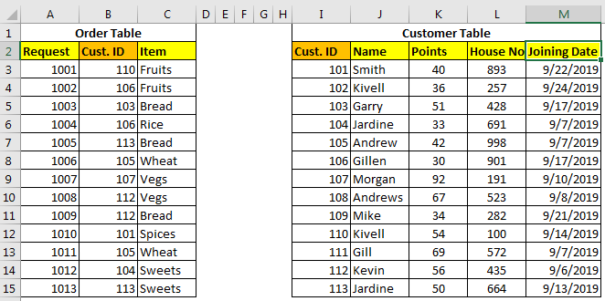
The Order Table has order details and the Customer table contains customer details. We need to prepare a table that tells which order belongs to which customer name, customer’s points, house number, and his joining date.
The common id in both tables is Cust.ID which can be used for merging tables in excel.
There are three methods of merging tables using VLOOKUP Function.
Retrieve Each Column With Column Index
In this method, we will use simple VLOOKUP to add these tables in one table. So to retrieve name write this formula.
[Customers is Sheet1!$I$3:$M$15.]
=VLOOKUP(B3,Customers,2,0)
To merge points in table, write this formula.
=VLOOKUP(B3,Customers,3,0)
To merge house no in table, write this formula.
=VLOOKUP(B3,Customers,4,0)

Here we merged two tables in excel, each column one by one in the table. This is useful when you have only few columns to merge. But when you have multiple columns to merge, this is can be a hectic task. So to merge multiple tables we have different approaches.
Merge Tables Using VLOOKUP and COLUMN Function.
When you want to retrieve multiple adjacent columns, use this formula.
=VLOOKUP(lookup_value,table_array,COLUMN()-n,0)
Here the COLUMN function just returns the column numbers in which the formula is being written.
n is any number which adjusts the column number in table array,
In our example, the formula for table merging will be:
=VLOOKUP($B3,Customers,COLUMN()-2,0)
Once you write this formula, you will not have to write the formula again for other columns. Just copy it in all other cells and columns.

How It Works
Ok! In the first column, we need a name, which is the second column in customer table.
Here the main factor is COLUMN()-2. The COLUMN function returns the column number of current cell. We are writing the formula in D3, hence we will get 4 from COLUMN(). Then we are subtracting 2 which makes 2. Hence finally our formula simplifies to =VLOOKUP($B3,Customers,2,0).
When we copy this formula in E columns we will get the formula as =VLOOKUP($B3,Customers,3,0). Which retrieves 3rd column from customer table.
Merge Tables Using VLOOKUP-MATCH Function
This one is my favorite way of merging tables in excel using the VLOOKUP function. In the above example, we retrieved column in serial. But what if we had to retrieve random columns. In that case above Techniques will be useless. The VLOOKUP-MATCH technique uses column headings to merge cells. This is also called VLOOKUP with Dynamic Col Index.
For our example here, the formula will be this.
=VLOOKUP($B3,Customers,MATCH(D$2,$J$2:$N$2,0),0)
Here, we are simply using MATCH function to get the appropriate column number. This called Dynamic VLOOKUP.
Using INDEX-MATCH to Table Merging in Excel
The INDEX-MATCH is very powerful lookup tool and many time it is referred as better VLOOKUP function. You can use this to for combining two or more tables. This will also allow you to merge columns from left of the table.
This was a quick tutorial about merging and joining tables in excel. We explored several ways of merging two or more tables in excels. Feel free to ask question about this article or any other query regarding excel 2019, 2016, 2013 or 2010 in the comments section below.
Related Articles:
IF, ISNA and VLOOKUP function in Excel
IFERROR and VLOOKUP function in Excel
How to retrieve the entire row of a matched value in Excel
Popular Articles :
50 Excel Shortcut to Increase Your Productivity : Get faster at your task. These 50 shortcuts will make you work even faster on Excel.
How to use the VLOOKUP Function in Excel : This is one of the most used and popular functions of excel that is used to lookup value from different ranges and sheets.
How to use the COUNTIF function in Excel : Count values with conditions using this amazing function. You don’t need to filter your data to count specific values. Countif function is essential to prepare your dashboard.
How to use the SUMIF Function in Excel : This is another dashboard essential function. This helps you sum up values on specific conditions.
Содержание
- Merge and unmerge cells
- Merge cells
- Unmerge cells
- Merge cells
- Unmerge cells
- Split text from one cell into multiple cells
- Merge cells
- Unmerge cells
- Need more help?
- How can I merge two or more tables?
- Merge two tables using the VLOOKUP function
- How to merge two or more tables in Excel
- How to merge two tables in Excel with formulas
- How to join tables with VLOOKUP
- How to merge tables in Excel with INDEX MATCH
- How to combine tables by matching multiple columns
- Join multiple tables into one with Excel Power Query
- Merge Tables Wizard — quick way to join tables by matching columns
- Example 1. Combine two tables by multiple columns
- Example 2. Join tables and update selected columns
- Example 3. Merge multiple matches from two tables
- Combine tables in Excel by column headers
- More tools to merge tables in Excel
- Available downloads
Merge and unmerge cells
You can’t split an individual cell, but you can make it appear as if a cell has been split by merging the cells above it.
Merge cells
Select the cells to merge.
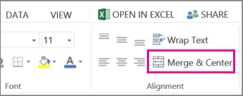
Select Merge & Center.
Important: When you merge multiple cells, the contents of only one cell (the upper-left cell for left-to-right languages, or the upper-right cell for right-to-left languages) appear in the merged cell. The contents of the other cells that you merge are deleted.
Unmerge cells
Select the Merge & Center down arrow.
Select Unmerge Cells.
You cannot split an unmerged cell. If you are looking for information about how to split the contents of an unmerged cell across multiple cells, see Distribute the contents of a cell into adjacent columns.
After merging cells, you can split a merged cell into separate cells again. If you don’t remember where you have merged cells, you can use the Find command to quickly locate merged cells.
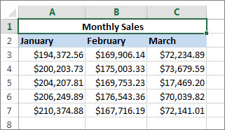
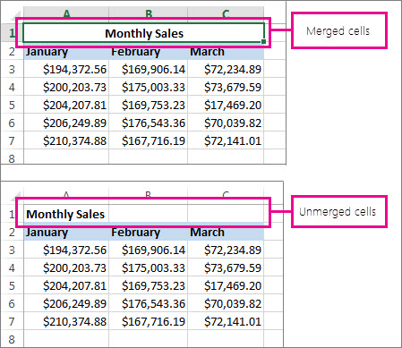
Merging combines two or more cells to create a new, larger cell. This is a great way to create a label that spans several columns.
In the example here, cells A1, B1, and C1 were merged to create the label “Monthly Sales” to describe the information in rows 2 through 7.
Merge cells
Merge two or more cells by following these steps:
Select two or more adjacent cells you want to merge.
Important: Ensure that the data you want to retain is in the upper-left cell, and keep in mind that all data in the other merged cells will be deleted. To retain any data from those other cells, simply copy it to another place in the worksheet—before you merge.
On the Home tab, select Merge & Center.
If Merge & Center is disabled, ensure that you’re not editing a cell—and the cells you want to merge aren’t formatted as an Excel table. Cells formatted as a table typically display alternating shaded rows, and perhaps filter arrows on the column headings.
To merge cells without centering, click the arrow next to Merge and Center, and then click Merge Across or Merge Cells.
Unmerge cells
If you need to reverse a cell merge, click onto the merged cell and then choose Unmerge Cells item in the Merge & Center menu (see the figure above).
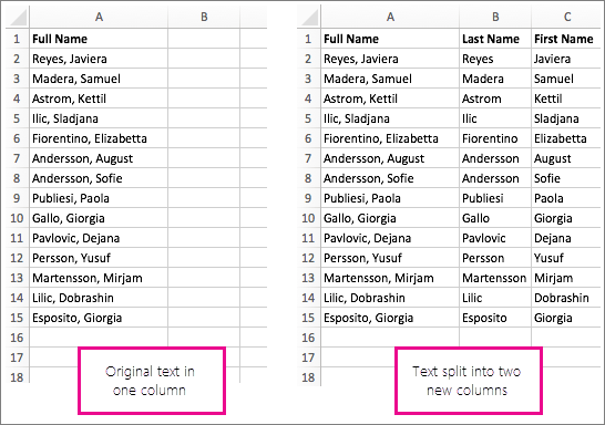
Split text from one cell into multiple cells
You can take the text in one or more cells, and distribute it to multiple cells. This is the opposite of concatenation, in which you combine text from two or more cells into one cell.
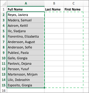
For example, you can split a column containing full names into separate First Name and Last Name columns:
Follow the steps below to split text into multiple columns:
Select the cell or column that contains the text you want to split.
Note: Select as many rows as you want, but no more than one column. Also, ensure that are sufficient empty columns to the right—so that none of your data is deleted. Simply add empty columns, if necessary.
Click Data > Text to Columns, which displays the Convert Text to Columns Wizard.
Click Delimited > Next.
Check the Space box, and clear the rest of the boxes. Or, check both the Comma and Space boxes if that is how your text is split (such as «Reyes, Javiers», with a comma and space between the names). A preview of the data appears in the panel at the bottom of the popup window.
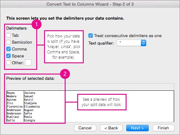
Click Next and then choose the format for your new columns. If you don’t want the default format, choose a format such as Text, then click the second column of data in the Data preview window, and click the same format again. Repeat this for all of the columns in the preview window.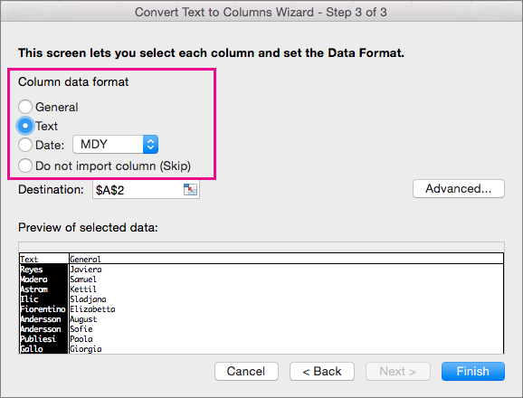
Click the  button to the right of the Destination box to collapse the popup window.
Anywhere in your workbook, select the cells that you want to contain the split data. For example, if you are dividing a full name into a first name column and a last name column, select the appropriate number of cells in two adjacent columns.
Click the  button to expand the popup window again, and then click the Finish button.

Merging combines two or more cells to create a new, larger cell. This is a great way to create a label that spans several columns. For example, here cells A1, B1, and C1 were merged to create the label “Monthly Sales” to describe the information in rows 2 through 7.
Merge cells
Click the first cell and press Shift while you click the last cell in the range you want to merge.
Important: Make sure only one of the cells in the range has data.
Click Home > Merge & Center.
If Merge & Center is dimmed, make sure you’re not editing a cell or the cells you want to merge aren’t inside a table.
Tip: To merge cells without centering the data, click the merged cell and then click the left, center or right alignment options next to Merge & Center.
If you change your mind, you can always undo the merge by clicking the merged cell and clicking Merge & Center .
Unmerge cells
To unmerge cells immediately after merging them, press Ctrl + Z. Otherwise do this:
Click the merged cell and click Home > Merge & Center.
The data in the merged cell moves to the left cell when the cells split.
Need more help?
You can always ask an expert in the Excel Tech Community or get support in the Answers community.
Источник
How can I merge two or more tables?
You can merge (combine) rows from one table into another simply by pasting the data in the first empty cells below the target table. The table will increase in size to include the new rows. If the rows in both tables match up, you can merge the columns of one table with another—by pasting them in the first empty cells to the right of the table. In this case also, the table will increase to accommodate the new columns.
Merging rows is actually quite simple, but merging columns can be tricky if the rows of one table don’t correspond with the rows in the other table. By using VLOOKUP, you can avoid some of the alignment problems.
Merge two tables using the VLOOKUP function
In the example shown below, you’ll see two tables that previously had other names to new names: «Blue» and «Orange.» In the Blue table, each row is a line item for an order. So, Order ID 20050 has two items, Order ID 20051 has one item, Order ID 20052 has three items, and so on. We want to merge the Sales ID and Region columns with the Blue table, based on matching values in the Order ID columns of the Orange table.
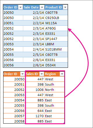
Order ID values repeat in the Blue table, but Order ID values in the Orange table are unique. If we were to simply copy-and-paste the data from the Orange table, the Sales ID and Region values for the second line item of order 20050 would be off by one row, which would change the values in the new columns in the Blue table.
Here’s the data for the Blue table, which you can copy into a blank worksheet. After you paste it into the worksheet, press Ctrl+T to convert it into a table, and then rename the Excel table Blue.
Источник
How to merge two or more tables in Excel
 by Svetlana Cheusheva, updated on March 16, 2023
In this tutorial, you will find some tricks on merging Excel tables by matching data in one or more columns as well as combining worksheets based on column headers.
When analyzing data in Excel, how often do you have all necessary information gathered in a single worksheet? Almost never! It is a very common situation when different pieces of data are dispersed across many worksheets and workbooks. Fortunately, there are a few different ways to combine data from multiple tables into one, and this tutorial will teach you how to do this quickly and effectively.
How to merge two tables in Excel with formulas
Whatever task you need to perform in your worksheets, where do you look for a solution in the first place? Like many users, I usually go to the Formulas tab and open a list of functions. Merging tables is no exception 🙂
How to join tables with VLOOKUP
If you are to merge two tables based on one column, VLOOKUP is the right function to use.
Supposing you have two tables in two different sheets: the main table contains the seller names and products, and the lookup table contains the names and amounts. You want to combine these two tables by matching data in the Seller column:
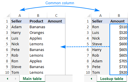
As you see, the order of the names in the main table does not correspond with that in the lookup table, therefore a simple copy/pasting technique won’t work.
To combine two tables by a matching column (Seller), you enter this formula in C2 in the main table:
- $A2 is the value you are looking for.
- ‘Lookup table’!$A$2:$B$10 is the table to search (please pay attention that we lock the range with absolute cell references).
- 2 is the number of the column from which to retrieve the value.
Copy the formula down the column, and you will get a merged table consisting of the main table, plus the matched data pulled from the lookup table:

Please be aware that Excel VLOOKUP has several limitations, the most critical of which are 1) inability to pull data from a column to the left of the lookup column and 2) a hardcoded column number breaks a formula when you add or remove columns in the lookup table. On the bright side, you can easily reorder the returned columns simply by changing the number in the col_index_num argument.
Tip. If you have an Excel 365 subscription, then you can use a more powerful successor of VLOOKUP — Excel XLOOKUP function.
How to merge tables in Excel with INDEX MATCH
If you are looking for a more powerful and versatile alternative to the VLOOKUP function, embrace this INDEX MATCH combination:
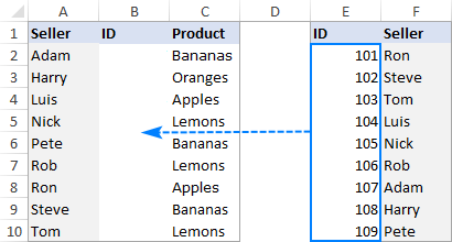
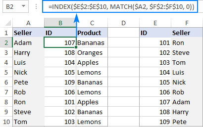
The syntax is explained in detail in this tutorial: INDEX / MATCH in Excel. And here I will show you how to use this formula to look up from right to left, something that VLOOKUP is unable to do.
Let’s say you have another lookup table with order IDs in the first column and you wish to copy those IDs to the main table by matching the seller names. For better visualization, both tables are put on the same sheet:
To accomplish the task, you supply the following arguments to the Index Match formula:
Please notice the $ sign that locks the ranges to prevent them from changing as you copy the formula down the table:
The completed formula looks as follows:
=INDEX($E$2:$E$10, MATCH($A2, $F$2:$F$10, 0))
…and combines data from two tables perfectly:
In Excel 365, you can use the new XLOOKUP function for the same purpose:
=XLOOKUP(A2, $F$2:$F$10, $E$2:$E$10, «Not found»)
How to combine tables by matching multiple columns
If the two tables you wish to join do not have a unique identifier, such as an order id or SKU, you can match values in two or more columns by using this formula:
Note. It is an array formula, so please remember to press Ctrl + Shift + Enter to enter it correctly.
The formula’s breakdown can be found here: Look up with multiple criteria. For now, let’s focus on the practical usage.
Assuming you have the following two tables to be combined into one. Because the Order ID column is missing in the lookup table, the only way to match the orders is by Seller and Product:

Based on the above screenshot, let’s define the arguments for our formula:
Again, be sure to fix all the ranges with absolute cell references so that they won’t change when you copy the formula down:
=INDEX($F$2:$H$9, MATCH(1, ($B2=$F$2:$F$9) * ($C2=$G$2:$G$9), 0), 3)
Enter the formula in D3, press Ctrl + Shift + Enter , copy it to the below rows and check the result:

To have a closer look at the above examples and probably reverse-engineer the formulas, you are welcome to download our sample workbook to Merge Two Tables in Excel.
Join multiple tables into one with Excel Power Query
In situations when you need to combine two or more tables with different numbers of rows and columns, Excel Power Query may come in handy. However, please be aware that joining tables with Power Query cannot be done with a mere couple of clicks. Explaining all the nuances would take far more space than we have here, so I will just briefly outline the main features:
- Power Query can merge two tables by matching one or several columns.
- The source tables can be on the same sheet or in different worksheets.
- The original tables are not changed. The data is combined into a new table that can be imported in an existing or a new worksheet.
- In Excel 2016 — Excel 365, Power Query is an inbuilt feature. In Excel 2010 and Excel 2013, it can be downloaded as an add-in.
The detailed guidance can be found in this tutorial: How to join tables with Excel Power Query.
Merge Tables Wizard — quick way to join tables by matching columns
If you are not very comfortable with Excel formulas yet, nor do you have time to figure out the arcane quirks of Power Query, our Merge Tables Wizard could be your time-saver. Below I will show three most popular uses cases.
Example 1. Combine two tables by multiple columns
If you find the array formula for columns match hard to remember, rely on our add-in to do the job quickly and perfectly.
For this example, we will be using the already familiar tables and join them based on 2 columns, Seller and Product. Please note that the lookup table has 2 more columns than the main table:

With the Merge Tables Wizard added to your Excel ribbon, here’s what you need to do:
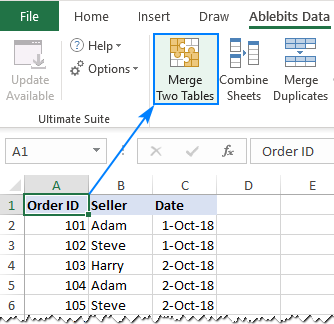
- Select any cell within your main table and click the Merge Two Tables button on the Ablebits Data tab:
Make sure the add-in got the range right, and click Next:

Select the lookup table, and click Next:

Specify the column pairs to match, Seller and Product in our case, and click Next:

Tip. If the text case in the key columns matters, check the Case-sensitive matching box to treat uppercase and lowercase as different characters.

Select the columns to add to the main table and click Next.

The default options work just fine in our case, so we click Finish without changing anything:

Allow the wizard a few seconds for processing and review the result:
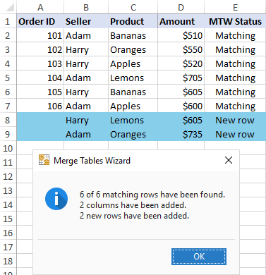
As you can see in the screenshot above, the wizard has done the following:
- Added the Amount column by matching the seller name and product in both tables.
- Added the Status column that allows you to easily filter matching and new rows. If you don’t want it, clear the corresponding box in the final step.
- New rows that were present only in the lookup table were copied to the end and highlighted in blue.
- If you don’t want to highlight new rows, unselect Set background color for all added rows in the last step.
- If you don’t want to add new rows, unselect Add non-matching rows to the end of the main table in the last step.
Example 2. Join tables and update selected columns
In case your main table contains some outdated data, you can have it updated with the corresponding values from the lookup table.
As an example, let’s merge 2 tables by Order ID and update the values in the Price column:

To get the result shown in the above image, this is what you need to do:
Step 1. Select the main table.
Step 2. Select the lookup table.
Step 3. Choose Order ID as the matching column.
Step 4. Select Price as the column to update.
Step 5. Skip it because there are no columns to add.
Step 6. Since there are a few gaps in the New price column, we choose to update only if cells in the lookup table contain data. Optionally, you can highlight the updated cells with any color of your choosing. The screenshot below shows the settings:

Tip. To prevent overwriting your existing data, you can update only empty cells in the main table.
Example 3. Merge multiple matches from two tables
In situations when a lookup table contains several occurrences on the lookup value, you may want to pull them all to your main table. The task can be accomplished with one of the non-trivial array formulas described in Vlookup to return multiple matches in Excel. Or you can do it the easy way with the Merge Tables Wizard.
Supposing your main table contains just one order of each seller, and the lookup table contains additional orders. Now you want to combine all the orders in one table, grouped by seller name like this:

Looks like a lot of work to do? Not if you have the Merge Tables Wizard at your disposal 🙂
Step 1. Select the main table.
Step 2. Select the lookup table.
Step 3. Choose Seller as the column to match.
Step 4. Update Order ID and Product.
Step 5. There are no columns to add.
Step 6. Insert additional matching rows after the row with the same key value. Optionally, set a background color for added rows to review the changes with a quick glance:

The above examples show just 3 of many possible ways to join tables in Excel. If you are curious to see other scenarios that the Merge Table Wizards can handle, please check out the visuals on this page. Or you can download a 30-day trial version and give it a shot.
Combine tables in Excel by column headers
In the above examples, we were merging two tables that have identical columns and pulling data from one table to another. In case you want to join multiple tables from different sheets into one based on columns headers, our Combine Sheets add-in is the right tool for the job.
The below image shows the source tables and desired result:

And here’s how you can accomplish the task:
- On your Excel ribbon, go to the Ablebits tab >Merge group, and click the Combine Sheets button:

Select all the worksheets you want to merge into one.
If you’d like to combine just one table, not all data, hover over the sheet’s name, and then click the Collapse dialog icon on the right to select a range:

Choose the columns you want to combine, Order ID and Seller in this example:

Select additional options, if needed. We go with the default ones that work perfectly in most cases:

Finally, specify where you want to put the resulting table, and click Combine:

Done! The three tables are combined into one exactly like shown in the beginning of this example.
The Merge Tables Wizard and Combine Sheets are the most popular tools to join tables in Excel. If you have some other task in mind, chances are that you will also find a quick solution on the Ablebits Data tab:

Let me briefly describe what each of these add-ins does:
Merge Two Tables — joins two tables that have one or more identical columns, as shown in these examples.
Combine Sheets — merges multiple worksheets into one based on column headers, like we did a moment ago in this example.
Merge Duplicates — combines duplicate rows by key columns.
Consolidate Sheets — joins tables together and summarizes their data.
Copy Sheets — provides 4 different ways to merge sheets in Excel.
Merge Cells — merge cells, columns, and rows without losing data, even if a selection contains multiple values.
Vlookup Wizard — quick way to build a Vlookup or Index/Match formula best suited for your data set.
Compare Sheets — find, highlight, and merge differences between two worksheets.
Compare Multiple Sheets — highlight differences in two or more sheets.
All the above features as well as 70+ other time-saving tools are included with our Ultimate Suite for Excel. An evaluation version is available for download right below this post. I thank you for reading and hope to see you on our blog next week!
Available downloads
Table of contents
I have a sheet that has various tabs with same columns, but I need to add a *new column from TAB A to the rest of the TABS based a the description of the *rest of the tabs’ columns.
If; Where new column named CODE on the rest of the TABS = the input of column named CODE (but also match the input of the column named DESCRIPTION, which mirror/replicate the input rest of the tabs.)
TAB A
HEADER COLUMNS= Visit>Visit ABRV> CODE>DESCPT
REST OF TABS
*NEW COLUMN (CODE) = when DESCPT from TAB A matches DESCPT column from *rest of tabs on the sheet.
Hello!
To solve your problem, I recommend using the Merge Tables Wizard, as described in the article above.
I have a question regarding INDEX/MATCH. It seems to mostly work for me, however when I try to extend the formula downwards, it changes the INDEX array and MATCH lookup array selection downwards. Here’s an example:
For the 1st value (in 2nd row) I use the following formula: INDEX(G2:G5284;MATCH(A2;F2:F5284;0))
For the 2nd value the formula then becomes: =INDEX(G3:G5284;MATCH(A3;F3:F5284;0))
where what I’d want is INDEX(G2:G5284;MATCH(A3;F2:F5284;0))- change in lookup value but not the array.
This is a problem, because many of the outputs will then become #N/A- the lookup value will fall outside the lookup array. I tried to fix this by manually editing the first few formulas and extending the formulas downwards, but that doesn’t work. Does anyone have a fix for that?
Hello!
Try to use the recommendations described in this article: How to copy formula in Excel with or without changing references.
Please try the following formula:
I have two sheets. Sheet2 has 1741 rows and Sheet1 has 324. Sheet1 column A has id numbers that all exist in Sheet2 column D. I want to append the text cells (Columns $B:$H) from sheet1 to the matching rows in sheet2. I have tried multiple formulas and keep getting error with formula messages. I have tried using vlookup in different forms including from the above:
=VLOOKUP($D2,’sheet1′!$A2$H324,2,FALSE)
But that calculates some number that I have no idea where it came from.
Hello!
For column B you can use this formula:
We have tools that can solve your task in a couple of clicks — Vlookup Wizard and Merge Two Tables. It is available as a part of our Ultimate Suite for Excel that you can install in a trial mode and check how it works for free
can anyone help me for excel
A B C D E
456 ram ram 456 345
345 ram shyam 213 545
213 shyam krishna 548 724
545 shyam
548 krishna
724 krishna
I want a result in column B if column A is equal to column D and column E
then i want a result in column B with name ram shyam krishna
Hi!
I don’t really understand what conditions you want to use, but this article will help you: Excel IF statement with multiple AND/OR conditions.
In «sheet1» I have this format says
rows Cell A1=Employee Names referring to cell B1=John, cell F1=Maria, cell G1=Peter & cell K1=Mark
now in «Sheet2» I want to lookup those Employee Names resulting in this format says column cell A1=John, cell A2=Maria, cell A3=Peter, cell A4=Mark.
Is there any formula to consolidate those names? Thanks
Hello!
You cannot consolidate rows and columns. Therefore, on Sheet 2, you need to perform the Transpose operation. You can then merge the column data on both sheets using the Consolidate Sheets or Combine Sheets tools.
I hope I answered your question. If something is still unclear, please feel free to ask.
Hi Svetlana Cheusheva
I have six sheets that have purchases of six companies, the amount of data is huge one of these sheets has over 70000 rows of data. my goal is to extract the mutual purchases items only between these companies. is there any way to do this because I have tried many ways to do so but I haven’t managed.
Thanks in advance for your time and effort
Dear Svetlana,
Thankyou for this it is very helpful. Could you guide me on the appropriate option for my below issue.
I have a file(ytd) that I need to update monthly, with monthly figures. So my file that needs to be updated has 3 columns with data, now to this data/figures I need to add the monthly figures and arrive at the the updated total figures ytd.
YTD file Column1 =5
MTD file Column1 =3
Updated YTD file Column1 =8
Please guide.
I am a full noob !
I have suppliers who have given me tables with door models on the top row sizes down the left column and pricing to the right column under the door models
How do i combine these tables to read read :
Door model, door size, and door price so i can import these items into my catalogue.
I have searched everywere — in the past i have used concatenate but there must be an easier way to combine 20000 plus items a section at a time ? This information will be LIFE CHANGING to me, thanks in advance ! I am trying my best !
Hello George!
I hope you have studied the recommendations in the above tutorial. We have a tool that can solve your task in a couple of clicks: Ablebits Data — Merge Tables.
This tool is available as a part of our Ultimate Suite for Excel that you can install in a trial mode and use for free: https://www.ablebits.com/files/get.php?addin=xl-suite&f=free-trial
Unfortunately, without seeing your data it is impossible to give you advice.
I’m sorry, it is not very clear what result you want to get. Could you please describe your task in more detail and send us a small sample workbook with the source data and expected result to support@ablebits.com? Please shorten your tables to 10-20 rows/columns and include the link to your blog comment.
We’ll look into your task and try to help.
Is there a size limit to your combine tables add in? I’ve got a couple data tables with
3,700 rows. I need to join 2 such tables each with about 10 columns. A numeric code is the common column between them.
Can you please update this guide to also include the steps to merge tables using the new XLOOKUP function as an alternative to VLOOKUP and INDEX/MATCH?
It’s an excellent suggestion, thank you! I have added an XLOOKUP formula to the INDEX/MATCH example. As soon as I have a little more time, I will try to describe it in more detail.
In the meantime, you can take a look at our XLOOKUP tutorial that covers a lot of interesting use cases. Hopefully, you’ll find the examples useful.
I have two tables like with these records:
Table 1: Badge# | Name | EmployeeID
Table 2: EmployeeID | SchoolID | Name | Badge#
Is there any ways that I can get the badge# record from table1 to the badge# in table 2 with the matching EmployeeID.
Thank you.
Hello,
I have been trying to combine a couple of sheet with one common value, how would you combine this:
If Sheet1!A1 = Sheet2!B2 then combine Sheet2!C2:sheet2!I15
Thanks in advance!
Just came across this article. Looks like a very old question but in case anyone else has the same thought, first ask yourself: If I have a one to many relationship I want to join, could I perhaps have the LOOKUP on the MANY side instead of the ONE, to yield the same result.
Not sure your data structure or if the rows are fixed. You have many possible routes. If your goal (for example) is to use a one to many relationship and list all matches from sheet2 in columns to the right of sheet1, combining multiple columns into each cell, you might do this:
Sheet 1 — Match values (ie names) in column A starting cell A2. Target columns for dropping results and entering formula starting D2.
Sheet 2 — Match values (ie names) in column A starting cell A3. A date column in B and a text value in C.
hey there;
I have a question, is there any way to overlay tables like he following;
table 1;
monday tues wed thurs friday
10 m10 t10 w1o th10 fri10
11 m11 t11 w11 th11 fri11
12 m12 t12 w12 th12 fri12
13 m13 t13 w13 th13 fri13
table 2;
monday tues wed thurs friday
10 M10 T10 W1o TH10 FRI10
11 M11 T11 W11 TH11 FRI11
12 M12 T12 W12 TH12 FRI12
13 M13 T13 W13 TH13 FRI13
and get the resulting table:
monday tues wed thurs friday
10 m10 t10 w1o th10 fri10
M10 T10 W1o TH10 FRI10
11 m11 t11 w11 th11 fri11
M11 T11 W11 TH11 FRI11
12 m12 t12 w12 th12 fri12
M12 T12 W12 TH12 FRI12
13 m13 t13 w13 th13 fri13
M13 T13 W13 TH13 FRI13
Hi,
I was wondering if it was possible to put the Merge Two Tables feature in a macro or VBA script? I have to do this process multiple times a month and I’d like to automate it.
tHANK YOU VERY MUCH
Amazing Add-in! Thank you very much for still developing this very useful and resourceful tool, Keep it up! =)
Hi,
I have a question. I just bought the add-in but I am unable to figure out what I want to do.
I have excel sheets for each projects I am working on.
Sheet Project A
Table1, Columns: Task, Assigned to, Start date, Due date, Status
Sheet Project B
Table2, Columns: Task, Assigned to, Start date, Due date, Status
Sheet Project C
Table3, Columns: Task, Assigned to, Start date, Due date, Status
And now I want to view all the tasks created in these three tables on 1 single table.
Could you tell me how to do it?
Best regards,
Baatarbat
Hi Svetlana,
I read your posts with interest. I hope you can help me with my query:
I have three one-column tables and wish to create a new 3-column table combining them in the following way:
TableA:
Item_A1
Item_A2
Item_A3
TableB:
Item_B1
Item_B2
TableC:
Item_C1
Item_C2
Item_C3
Item_C4
NewTable:
Item_A1 Item_B1 Item_C1
Item_A1 Item_B1 Item_C2
Item_A1 Item_B1 Item_C3
Item_A1 Item_B1 Item_C4
Item_A1 Item_B2 Item_C1
Item_A1 Item_B2 Item_C2
Item_A1 Item_B2 Item_C3
Item_A1 Item_B2 Item_C4
Item_A2 Item_B1 Item_C1
Item_A2 Item_B1 Item_C2
Item_A2 Item_B1 Item_C3
Item_A2 Item_B1 Item_C4
Item_A2 Item_B2 Item_C1
Item_A2 Item_B2 Item_C2
Item_A2 Item_B2 Item_C3
Item_A2 Item_B2 Item_C4
Item_A3 Item_B1 Item_C1
Item_A3 Item_B1 Item_C2
Item_A3 Item_B1 Item_C3
Item_A3 Item_B1 Item_C4
Item_A3 Item_B2 Item_C1
Item_A3 Item_B2 Item_C2
Item_A3 Item_B2 Item_C3
Item_A3 Item_B2 Item_C4
Please note that the number of rows in each of the three tables are dynamic and populated from SQL server queries. So, a copy/paste method is not practical. I think Power Query is the best approach but I don’t how.
I need to publish/send reports based on the new table. So, if your «Ultimate Suite» provides a solution for me, does it need to be installed on the remote computers too?
Many thanks for your help.
Abbas
Hi Abbas,
I regret to tell you that none of our tools can help with this task. I am not sure that even Power Query can do that, at least I don’t know a way. Sorry 🙁
Hi Abbas did you figure out how to do this?
Источник