
Combine text from two or more cells into one cell
You can combine data from multiple cells into a single cell using the Ampersand symbol (&) or the CONCAT function.

Combine data with the Ampersand symbol (&)
-
Select the cell where you want to put the combined data.
-
Type = and select the first cell you want to combine.
-
Type & and use quotation marks with a space enclosed.
-
Select the next cell you want to combine and press enter. An example formula might be =A2&» «&B2.
Combine data using the CONCAT function
-
Select the cell where you want to put the combined data.
-
Type =CONCAT(.
-
Select the cell you want to combine first.
Use commas to separate the cells you are combining and use quotation marks to add spaces, commas, or other text.
-
Close the formula with a parenthesis and press Enter. An example formula might be =CONCAT(A2, » Family»).
Need more help?

See also
TEXTJOIN function
CONCAT function
Merge and unmerge cells
CONCATENATE function
How to avoid broken formulas
Automatically number rows
Need more help?
Want more options?
Explore subscription benefits, browse training courses, learn how to secure your device, and more.
Communities help you ask and answer questions, give feedback, and hear from experts with rich knowledge.
Содержание
- How to merge two columns in Excel without losing data
- Merge two columns using Excel formulas
- Combine columns data via Notepad
- Join columns using the Merge Cells add-in for Excel
- How to combine two columns in 3 simple steps
- How to join tables in Excel: Power Query vs. Merge Tables Wizard
- How to join tables with Excel Power Query
- Source data
- Create Power Query connections
- Merge two connections into one table
- Select the columns to add from the second table
- Merge more tables (optional)
- Import the merged table to Excel
- How to join tables based on multiple columns with Power Query
- How to update/refresh the merged table
- Merge Tables Wizard — quick way to join 2 tables in Excel
- Other ways to combine data in Excel:
How to merge two columns in Excel without losing data
 by Alexander Frolov, updated on February 7, 2023
From this short article you will learn how to merge multiple Excel columns into one without losing data.
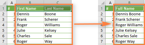
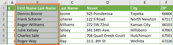
You have a table in Excel and what you want is to combine two columns, row-by-row. For example, you want to merge the First Name & Last Name columns into one, or join several columns such as Street, City, Zip, State into a single «Address» column, separating the values with a comma so that you can print the addresses on envelops later.
Regrettably, Excel does not provide any built-in tool to achieve this. Of course, there is the Merge button («Merge & Center» etc.), but if you select 2 adjacent cells in order to combine them, as shown in the screenshot:
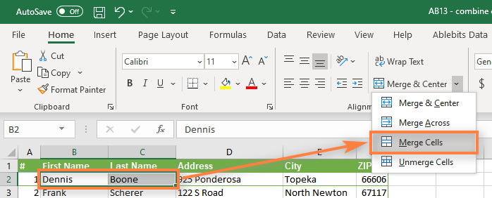
You will get the error message «Merging cells only keeps the upper-left cell value, and discards the other values.» (Excel 2013) or «The selection contains multiple data values. Merging into one cell will keep the upper-left most data only.» (Excel 2010, 2007)

Further in this article, you will find 3 ways that will let you merge data from several columns into one without losing data, and without using VBA macro. If you are looking for the fastest way, skip the first two, and head over to the 3rd one straight away.
Merge two columns using Excel formulas
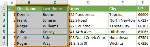
Say, you have a table with your clients’ information and you want to combine two columns (First & Last names) into one (Full Name).
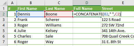
- Insert a new column into your table. Place the mouse pointer in the column header (it is column D in our case), right click the mouse and choose «Insert» from the context menu. Let’s name the newly added column «Full Name«.

In cell D2, write the following CONCATENATE formula:
In Excel 2016 — Excel 365, you can also use the CONCAT function for the same purpose:
Where B2 and C2 are the addresses of First Name and Last Name, respectively. Note that there is a space between the quotation marks » « in the formula. It is a separator that will be inserted between the merged names, you can use any other symbol as a separator, e.g. a comma.
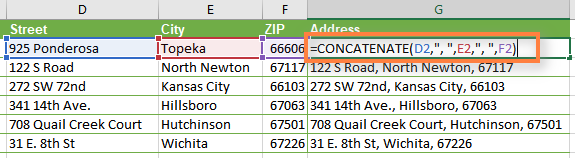
In a similar fashion, you can join data from several cells into one, using any separator of your choice. For instance, you can combine addresses from 3 columns (Street, City, Zip) into one.

Now we need to convert the formula to a value so that we can remove unneeded columns form our Excel worksheet. Select all cells with data in the merged column (select the first cell in the «Full Name» column, and then press Ctrl + Shift + ArrowDown ).
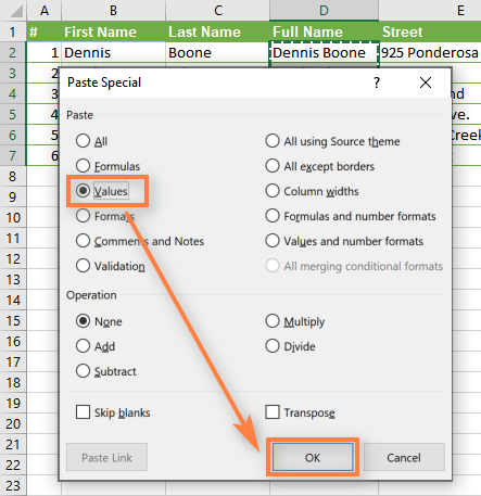
Copy the contents of the column to clipboard ( Ctrl + C or Ctrl + Ins , whichever you prefer), then right click on any cell in the same column («Full Name» ) and select «Paste Special» from the context menu. Select the Values button and click OK.
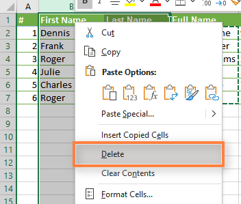
Remove the «First Name» & «Last Name» columns, which are not needed any longer. Click the column B header, press and hold Ctrl and click the column C header (an alternative way is to select any cell in column B, press Ctrl + Space to select the entire column B, then press Ctrl + Shift + ArrowRight to select the whole column C).
After that right click on any of the selected columns and choose Delete from the context menu:
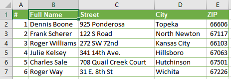
Fine, we have merged the names from 2 columns into one! Though, it did require some effort 🙂
Combine columns data via Notepad
This way is faster than the previous one, it doesn’t require formulas, but it is suitable only for combining adjacent columns and using the same delimiter for all of them.
Here is an example: we want to combine 2 columns with the First Names and Last Names into one.
- Select both columns you want to merge: click on B1, press Shift + Right Arrrow to select C1, then press Ctrl + Shift + Down Arrow to select all the cells with data in two columns.

Press Ctrl + H to open the «Replace» dialog box, paste the Tab character from the clipboard in the «Find what» field, type your separator, eg. Space, comma etc. in the «Replace with» field. Press the «Replace All» button; then press «Cancel» to close the dialog box.

There are more steps than in the previous option, but believe me or try it yourself — this way is faster. The next way is even faster and easier 🙂
Join columns using the Merge Cells add-in for Excel
The quickest and easiest way to combine data from several Excel columns into one is to use Merge Cells add-in for Excel included with our Ultimate Suite for Excel.
With the Merge Cells add-in, you can combine data from several cells using any separator you like (e.g. space, comma, carriage return or line break). You can join values row by row, column by column or merge data from the selected cells into one without losing it.
How to combine two columns in 3 simple steps
- Download and install the Ultimate Suite.
- Select all cells from 2 or more columns that you want to merge, go to the Ablebits.com Data tab > Merge group, and click Merge Cells >Merge Columns into One.
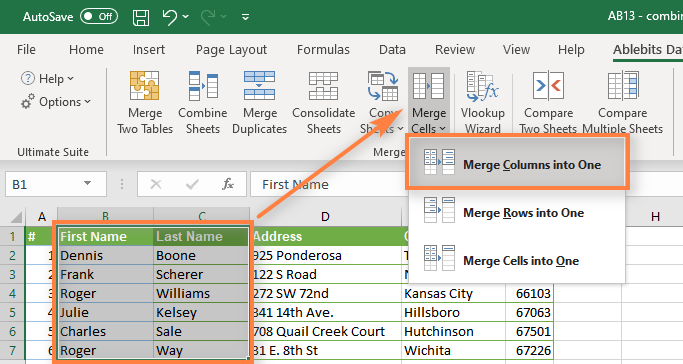
- How to merge: columns into one (preselected)
- Separate values with: choose the desired delimiter (space in our case)
- Place the results to: left column
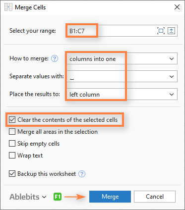
That’s it! A few simple clicks and we’ve got two columns merged without using any formulas or copy/pasting.
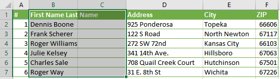
To finish up, rename column B to Full Name and delete column «C», which is not needed any longer.
Much easier than the two previous ways, isn’t it? 🙂
Источник
How to join tables in Excel: Power Query vs. Merge Tables Wizard
 by Svetlana Cheusheva, updated on March 16, 2023
In this tutorial, we will look at how you can join tables in Excel based on one or more common columns by using Power Query and Merge Tables Wizard.
Combining data from multiple tables is one of the most daunting tasks in Excel. If you decide to do it manually, you may spend hours only to find out that you’ve messed up important information. If you are an experienced Excel pro, then you can possibly rely on VLOOKUP and INDEX MATCH formulas. A macro, you believe, could do the job in no time, if only you knew how. The good news for all Excel users — Power Query or Merge Tables Wizard can be your time-saver. The choice is yours.
How to join tables with Excel Power Query
In simple terms, (also known as Get & Transform is a tool to combine, clean and transform data from multiple sources into the format you need such as a table, pivot table or pivot chart.
Among other things, Power Query can join 2 tables into 1 or combine data from multiple tables by matching data in columns, which is the focus of this tutorial.
For the results to meet your expectations, please keep in mind the following things:
- Power Query is a built-in feature in Excel 2016 — Excel 365, but it can also be downloaded in Excel 2010 and Excel 2013 and used as an add-in. In your version, some windows may look different from the images in this tutorial that were captured in Excel 2016.
- For the tables to be combined correctly, they should have at least one common column (also referred to as a common id or key column or unique identifier). Also, the common columns should contain only unique values, with no repeats.
- The source tables can be located on the same sheet or in different worksheets.
- Unlike formulas, Power Query does not pull data from one table to another. It creates a new table that combines data from the original tables.
- The resulting table does not update automatically. You should explicitly tell Excel to do this. Please see how to refresh a merged table.
Source data
As an example, let’s join 3 tables based on the common columns Order ID and Seller. Please note that our tables have different numbers of rows, and although table 1 has duplicates in the Seller column, table 3 contains only unique entries. 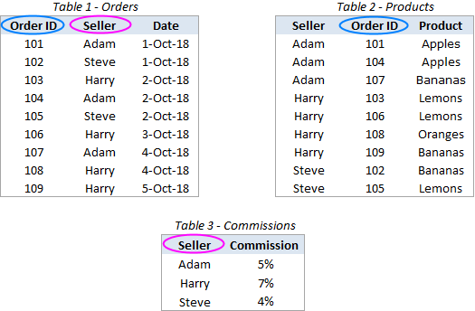
Our task is to map the data in table 1 with the relevant records from the other two tables, and combine all the data into a new table like this: 
Before you start joining, I’d advise you to give some descriptive names to your tables, so it will be easier for you to recognize and manage them later. Also, although we say «tables», you do not actually need to create an Excel table. Your «tables» could be usual ranges or named ranges as in this example:
- Table 1 is named Orders
- Table 2 is named Products
- Table 3 is named Commissions
Create Power Query connections
Not to clutter your workbook with copies of your original tables, we are going to convert them into connections, do the merge within the Power Query Editor, and then load only the resulting table.
To save a table as a connection in Power Query, here’s what you do:
- Select your first table (Orders) or any cell in that table.
- Go to the Data tab >Get & Transform group and click From Table/Range.

- In the Power Query Editor that opens, click on the Close & Loaddrop-down arrow (not the button itself!) and select the Close and Load To… option.
- In the Import Data dialog box, select the Only Create Connection option and click OK.


This will create a connection with the name of your table/range and display that connection in the Queries & Connections pane that appears on the right-hand side of your workbook.
When finished, you will see all the connections on the pane: 
Merge two connections into one table
With the connections in place, let’s see how you can join two tables into one:
- On the Data tab, in the Get & Transform Data group, click the Get Data button, choose Combine Queries in the drop-down list, and click Merge:
- In the Merge dialog box, do the following:
- Select your 1st table (Orders) from the first drop-down.
- Select your 2nd table (Products) from the second drop-down.
- In both previews, click on the matching column (Order ID) to select it. The selected column will get highlighted in green.
- In the Join Kind drop-down list, leave the default option: Left Outer (all from first, matching from second).
- Click OK.


Upon completion of the above steps, the Power Query Editor will show your first table (Orders) with one additional column named like your second table (Products) added to the end. This additional column does not have any values yet, just the word «Table» in all the cells. But don’t feel discouraged, you did everything right, and we are going to fix that in a moment!
Select the columns to add from the second table
At this point, you have a table resembling the one in the screenshot below. To complete the merging process, perform the following steps within the Power Query Editor:
- In the added column (Products), click on the two-sided arrow in the header.
- In the box that opens, do this:
- Keep the Expand radio button selected.
- Unselect all columns, and then select only the column(s) you want to copy from the second table. In this example, we select only the Product column because our first table already has Seller and Order ID.
- Uncheck the Use original column name as prefix box (unless you want the column name to be prefixed with the table name from which this column is taken).
- Click OK.


As the result, you will get a new table that contains every record from your first table and the additional column(s) from the second table: 
If you need to merge only two tables, you may consider the work almost done and go load the resulting table in Excel.
Merge more tables (optional)
In case you have three or more tables to join, there is some more work for you to do. I will outline the steps briefly here, because you have already done all this when joining the first two tables:
- Save the table you’ve got in the previous step (shown in the screenshot above) as a connection:
- In the Power Query Editor, click Close & Load drop-down arrow and select Close and Load To….
- In the Import Data dialog box, select Only Create Connection, and click OK.
This will add one more connection, named Merge1, to the Queries & Connections pane. You can rename this connection if you want (right-click and select Rename in the pop-up menu). 
Combine Merge1 with your third table (Commissions) by performing these steps (Data tab >Get Data >Combine Queries > Merge).
The screenshot below shows my settings: 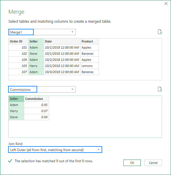
In this example, we add only the Commission column: 
As the result, you get a merged table that consists of the first table, plus the additional columns copied from the other two tables.
Import the merged table to Excel
With the resulting table in the Power Query Editor, there is just one thing left for you to do — load it in your Excel workbook. And it is the easiest part!
- In the Power Query Editor, click the Close & Load drop-down arrow, and choose Close and Load To….
- In the Import Data dialog box, select Table and New Worksheet options.
- Click OK.

A new table combining the data from two or more sources appears in a new worksheet. Congratulations, you did it!
As a finishing touch, you may want to apply the right number format to some columns and maybe change the default table style to your favorite one. After these improvements, my combined table looks very nice: 
Tip. If your tables contain numeric data (e.g. sales numbers or quantity) and you want a quick summary, you can load the resulting table as a PivotTable Report or create a pivot table in the usual way (Insert > PivotTable).
How to join tables based on multiple columns with Power Query
In the previous example, we were combining tables by matching data in one key column. But there is nothing that would prevent you from selecting two or more column pairs. Here’s how:
In the Merge dialog box, hold the Ctrl key and click on the key columns one-by-one to select them. It is important that you click on the columns in the same order in both previews, so the matching columns have the same numbers. For example, Seller is key column 1 and Product is key column 2. Blank cells or rows that Power Query is unable to match show null: 
After that, perform exactly the same steps as described above, and your tables will be merged by matching values in all the key columns.
How to update/refresh the merged table
The best thing about Power Query is that it is a one-time setup. When you make some changes to a source table, you don’t have to repeat the whole process again. Simply, click the Refresh button on the Queries & Connections pane, and the merged table will update at once: 
If the pane has disappeared from your Excel, click the Queries & Connections button on the Data tab to get it back.
Alternatively, you can click the Refresh all button on the Data tab tab or the Refresh button on the Query (this tab activates once you select any cell within a merged table).

Merge Tables Wizard — quick way to join 2 tables in Excel
Now that you are familiar with the inbuilt tool, let me show you our approach to merging tables in Excel.
In this example, we will be combining the same tables that we joined with Power Query a moment ago. I have just added a few more rows to the second table to show you more capabilities of our add-in: 
With the Merge Tables Wizard installed in your Excel, here’s what you need to do:
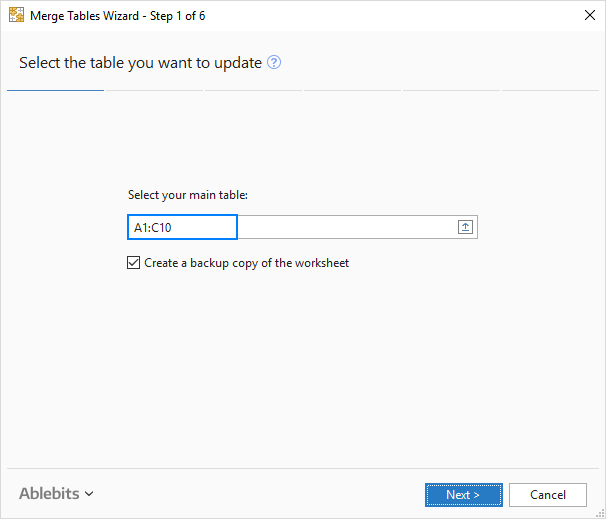
- Select the first table or any cell in it and click the Merge Two Tables button on the Ablebits Data tab:
- Take a quick look at the selected range to make sure the add-in got it right and click Next.
- Select the second table and click Next. Please note that our second table contains 26 rows compared to only 10 rows in the first table:
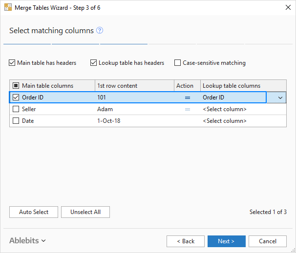
- Choose one or several matching columns and click Next. Since we are joining two tables by one common column, Order ID, we select only that column:
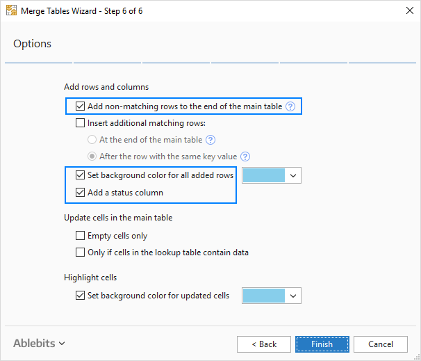
Please notice the Case-sensitive matching box at the top. Select it if you want to treat uppercase and lowercase text in the key columns as different characters. For this example, we don’t need that, so we leave the box unselected. - Select the columns to update in the first table. This step is optional, and if you don’t want any updates, you can click Next without selecting anything here.


We select the Seller column because we have more rows in the second table and we want the new seller names to appear in the existing Seller column: 

In this example, we go with the default options shown in the screenshot below. But I’d like to draw your attention to the following 2 boxes that can prevent overwriting your existing data in case you’ve chosen to update some columns:
- Empty cells only
- Only if cells in the lookup table contain data
Make your choices, click Finish, allow the wizard a few seconds for processing, and examine the results.
With the default options, the wizard highlights the newly added rows and adds the Status column. If you don’t want any of that, clear the corresponding boxes in the last step. 
To join three and more tables, simply repeat the above steps. Just remember to select the result of a previous merge as your main table.
Unlike Power Query, the Merge Tables Wizard does not keep a connection between the resulting and source tables. In some situations, this may be a disadvantage. On the plus side, no matter what you do with the source table — edit, move or even delete — the merged table remains intact.
This example has shown just one scenario that our wizard can handle, but there is much more to it! If you are curious to know other use cases, please check out these examples.
Also, you can download a a trial version of Ultimate Suite for Excel that includes Merge Tables Wizard as well as 70+ other useful tools.
In case you are looking to join tables in some other way, you may find the following resources useful.
Other ways to combine data in Excel:
Merge tables by column headers — join two or more tables based on column names. You can choose to combine all the columns or only the ones you select.
Combine multiple worksheets into one — copy multiple sheets into one summary worksheet. Of course, it’s not manual copy/pasting! You only indicate which worksheets to merge, and our Copy Sheets tool does the rest.
Compare two Excel files — how to compare two tables (worksheets) for differences and merge them into a single sheet.
Источник
Joining or merging two columns together in Excel is something every business owner will need to do eventually. If you’re importing data from another source, like a CSV file containing prospect names and contact information, the information is seldom going to be organized exactly as you need it. To merge data in Excel, including two or more columns, use the CONCAT or CONCATENATE formula. If you just need to merge two empty columns together, use Excel’s Merge option.
CONCAT vs. CONCATENATE in Excel
With Excel 2016, Microsoft replaced the CONCATENATE function with the CONCAT function. You can still use the CONCATENATE function, however Microsoft recommends using CONCAT. CONCATENATE may not be available in future versions of Excel. If you have an Office 365 subscription and can’t use the CONCAT function, update to the latest version of Excel.
Combine 2 Cells in Excel With CONCAT
The CONCAT function gives you the ability to combine the contents from one or more cells with any additional text you want. This usually makes it the perfect function when you want to join the contents of two or more columns.
Before you can combine two columns, you first need to combine the top two cells in each column. Once you have this done, you can quickly combine the rest of each column.
For example, suppose you imported a CSV file into Excel, with the first names in column A and surnames in column B. With CONCAT you can join them and arrange them anyway you want. Simply specify which cell goes first, the text you want (if any) in the middle, inside quotation marks, and then specify the second cell.
Example: A1 = Smith and B1 = John
In this example, the surname is in the first column, so if you want to have the surname after the first name, you need to select cell B1 first. A space needs to be inserted, within quotation marks, followed by cell A1:
John Smith =CONCAT(B1, » «, A1)
If you wanted the surname first, you can join the cells by placing a comma and then a space between the two cells:
Smith, John: =CONCAT(A1,», «, B1)
Combine 3 Cells in Excel With CONCAT
If you want to join three columns together, simply string them together with the text or spaces placed between.
Example: A1 = John, B1 = Smith, C1 = $400
John Smith Owes $400 =CONCAT(B1, » «, A1, » owes $», C1)
Note that in this example, the third column is formatted for currency. Because CONCAT strips the formatting from the cells, you will need to insert the $ yourself.
Combine Columns in Excel With CONCAT
To combine two columns in CONCAT, begin with the first cells in each column as described above. Once the cell appears the way you want it, you can copy it and paste it into the rest of the column.
First, highlight the cell containing the CONCAT formula and press Ctrl-C to copy it. Next, highlight all of the cells below that cell and press Ctrl-V to paste the formula. You’ll notice that Excel automatically changes the cell names in each row.
Once the new column of data has been created, you can delete the
Stripping the CONCAT Formula From a Column
Once the columns have been combined into a new column, you can remove the CONCAT formula and keep only the combined text, or values.
First, highlight the columns containing the source data and the new CONCAT column. Press Ctrl-C to copy.
Next, click the Home tab and then click the arrow below the Paste button in the Clipboard section of the ribbon. Click the «Paste Values» button.
With the formulas stripped from the column, you can now delete the columns you used to create it.
Merge Columns in Excel as Part of Formatting
Excel’s Merge option is useful for merging any group of cells, columns or rows that are adjacent to each other. When using Merge, however, all data except that in the upper-left cell will be deleted. This makes it a good option when you’re formatting a report or a business proposal for esthetic reasons, but not for combining cells that are full of data.
First highlight two or more columns, or rows or group of cells that are adjacent to each other. Then click the Home button and then click the «Merge and Center» button in the toolbar. Select «Merge Cells» from the drop-down options.
If you need to format the columns in addition to merging them, then right-click the highlighted cells, select «Format Cells.» Under the Alignment tab, you will see a checkbox to Merge cells.
If you’re using Excel and have data split across multiple columns that you want to combine, you don’t need to manually do this. Instead, you can use a quick and easy formula to combine columns.
We’re going to show you how to combine two or more columns in Excel using the ampersand symbol or the CONCAT function. We’ll also offer some tips on how to format the data so that it looks exactly how you want it.
How to Combine Columns in Excel
There are two methods to combine columns in Excel: the ampersand symbol and the concatenate formula. In many cases, using the ampersand method is quicker and easier than the concatenate formula. That said, use whichever you feel most comfortable with.
1. How to Combine Excel Columns With the Ampersand Symbol

- Click the cell where you want the combined data to go.
- Type =
- Click the first cell you want to combine.
- Type &
- Click the second cell you want to combine.
- Press the Enter key.
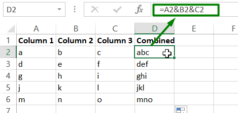
For example, if you wanted to combine cells A2 and B2, the formula would be: =A2&B2
2. How to Combine Excel Columns With the CONCAT Function

- Click the cell where you want the combined data to go.
- Type =CONCAT(
- Click the first cell you want to combine.
- Type ,
- Click the second cell you want to combine.
- Type )
- Press the Enter key.
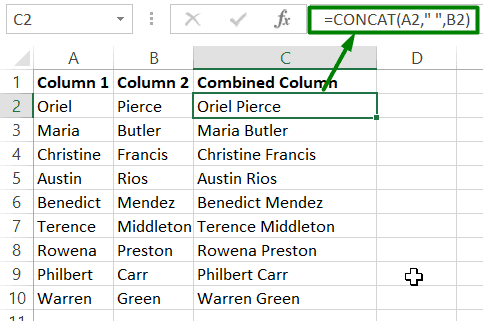
For example, if you wanted to combine cell A2 and B2, the formula would be: =CONCAT(A2,B2)
This formula used to be CONCATENATE, rather than CONCAT. Using the former works to combine two columns in Excel, but it is depreciating, so you should use the latter to ensure compatibility with current and future Excel versions.
How to Combine More Than Two Excel Cells
You can combine as many cells as you want using either method. Simply repeat the formatting like so:
- =A2&B2&C2&D2 … etc.
- =CONCAT(A2,B2,C2,D2) … etc.
How to Combine the Entire Excel Column
Once you have placed the formula in one cell, you can use this to automatically populate the rest of the column. You don’t need to manually type in each cell name that you want to combine.
To do this, double-click the bottom-right corner of the filled cell. Alternatively, left-click and drag the bottom-right corner of the filled cell down the column. It’s an Excel AutoFill trick to build spreadsheets faster.
Tips on How to Format Combined Columns in Excel
Your combined Excel columns could contain text, numbers, dates, and more. As such, it isn’t always suitable to leave the cells combined without formatting them.
To help you out, here are various tips on how to format combined cells. In our examples, we’ll refer to the ampersand method, but the logic is the same for the CONCAT formula.
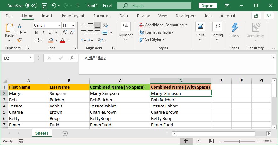
1. How to Put a Space Between Combined Cells
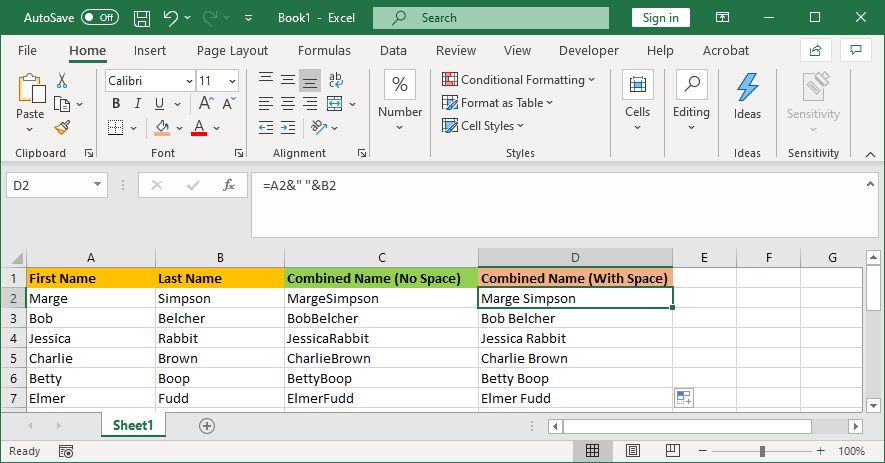
If you had a «First name» column and a «Last name» column, you would want a space between the two cells.
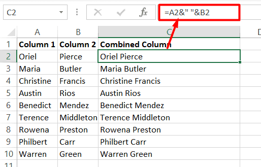
To do this, the formula would be: =A2&» «&B2
This formula says to add the contents of A2, then add a space, then add the contents of B2.
It doesn’t have to be a space. You can put whatever you want between the speech marks, like a comma, a dash, or any other symbol or text.
2. How to Add Additional Text Within Combined Cells
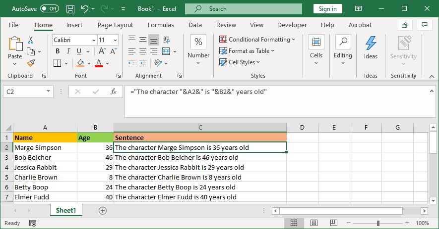
The combined cells don’t just have to contain their original text. You can add whatever additional information you want.
Let’s say cell A2 contains someone’s name (e.g., Marge Simpson) and cell B2 contains their age (e.g., 36). We can build this into a sentence that reads «The character Marge Simpson is 36 years old».
To do this, the formula would be: =»The character «&A2&» is «&B2&» years old»
The additional text is wrapped in speech marks and followed by an &. You don’t need to use speech marks when referencing a cell. Remember to include where the spaces should go; so «The character » with a space at the end.
3. How to Correctly Display Numbers in Combined Cells
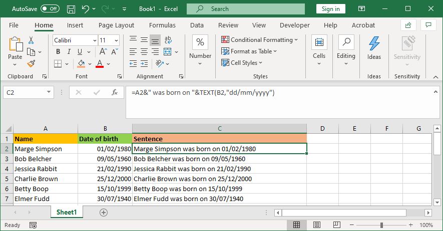
If your original cells contain formatted numbers like dates or currency, you’ll notice that the combined cell strips the formatting.
You can solve this with the TEXT function, which you can use to define the required format.
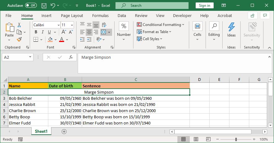
Let’s say cell A2 contains someone’s name (e.g., Marge Simpson) and cell B2 contains their date of birth (e.g., 01/02/1980).
To combine them, you might think to use this formula: =A2&» was born on «&B2
However, that’ll output: Marge Simpson was born on 29252. That’s because Excel converts the correctly formatted date of birth into a plain number.
By applying the TEXT function, you can tell Excel how you want the merged cell to be formatted. Like so: =A2&» was born on «&TEXT(B2,»dd/mm/yyyy»)
That’s slightly more complicated than the other formulas, so let’s break it down:
- =A2 — merge cell A2.
- &» was born on « — add the text «was born on» with a space on both sides.
- &TEXT — add something with the text function.
- (B2,»dd/mm/yyyy») — merge cell B2, and apply the format of dd/mm/yyyy to the contents of that field.
You can switch out the format for whatever the number requires. For example, $#,##0.00 would show currency with a thousand separator and two decimals, # ?/? would turn a decimal into a fraction, H:MM AM/PM would show the time, and so on.
You can find more examples and information on the Microsoft Office TEXT function support page.
How to Remove the Formula From Combined Columns
If you click a cell within the combined column, you’ll notice that it still contains the formula (e.g., =A2&» «&B2) rather than the plain text (e.g., Marge Simpson).
This isn’t a bad thing. It means that whenever the original cells (e.g., A2 and B2) are updated, the combined cell will automatically update to reflect those changes.
However, it does mean that if you delete the original cells or columns then it will break your combined cells. As such, you might want to remove the formula from the combined column and make it plain text.
To do this, right-click the header of the combined column to highlight it, then click Copy.
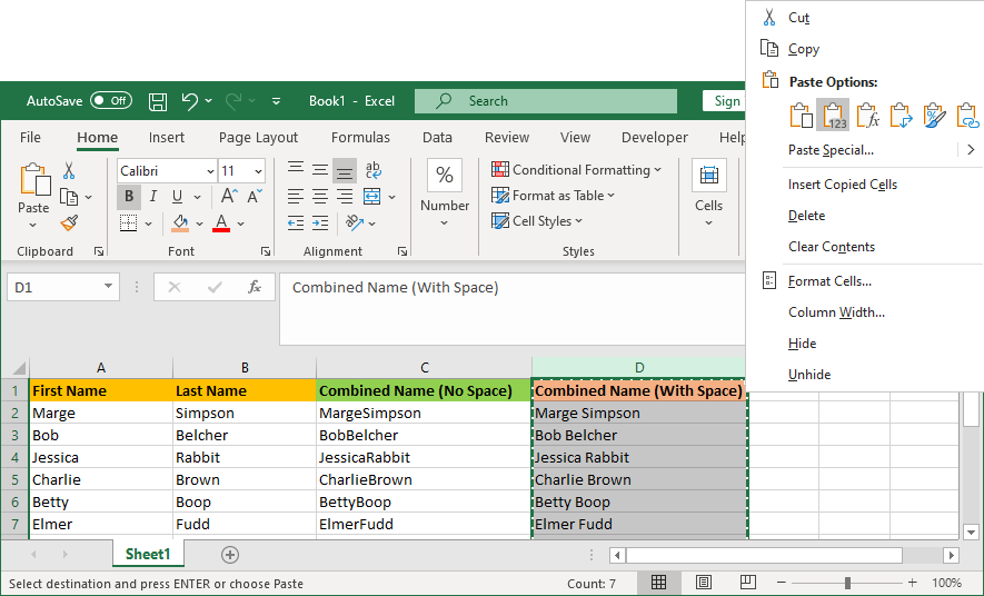
Next, right-click the header of the combined column again—this time, beneath Paste Options, select Values. Now the formula is gone, leaving you with plain text cells that you can edit directly.
How to Merge Columns in Excel
Instead of combining columns in Excel, you can also merge them. This will turn multiple horizontal cells into one cell. Merging cells only keeps the values from the upper-left cell and discards the rest.
To do this, select the cells or columns that you want to merge. In the Ribbon, on the Home tab, click the Merge & Center button (or use the dropdown arrow next to it).
For more information on this, read our article on how to merge and unmerge cells in Excel. You can also merge entire Excel sheets and files together.
Save Time When Using Excel
Now you know how to combine columns in Excel. You can save yourself lots of time—you don’t need to combine them by hand. It’s just one of the many ways that you can use formulas to speed up common tasks in Excel.
Note: This tutorial on how to combine two columns in Excel is suitable for all Excel versions including Office 365.
Manually merging columns in Excel can take a lot of time and effort. Here’s how to combine two columns in Excel the easy way.
In this article, you will learn:
- How to Combine Columns in Excel Sheets?
- How to Combine Two Columns in Excel With the CONCAT Function?
- How to Combine Two Columns in Excel With the Ampersand Symbol?
- How to Combine Multiple Columns in Excel into One column?
- How to Format Combined Columns in Excel?
- How to Insert a Space Between Combined Cells of the Columns?
- How to Correctly Display Dates and Currency in Combined Cells?
- How to Add Additional Text in Combined Cells?
- How to Remove the Formula from the Combined Columns?
- How to Merge Columns in Excel?
Related:
How To Protect Cells In Excel Workbooks-the Easiest Way
Excel Goal Seek—the Easiest Guide (3 Examples)
Create A Pivot Table In Excel—the Easiest Guide
How to Combine Columns in Excel Sheets?
Let’s say, for example, you have two separate columns containing the first and last names of your customers. Now, you want to combine these two columns into a single column that contains the full names of the customers.

There are two methods to go about doing this. You can either use the CONCAT formula method or use the ampersand method. Both of these methods are equally easy to use and I’ll break them down one by one in the following sections.
How to Combine Two Columns in Excel with the CONCAT Function?
- Click on the destination cell where you want to combine the two columns.
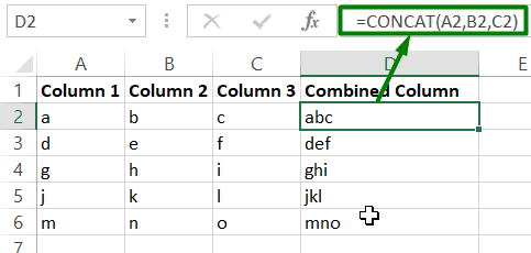
- Enter the formula: =CONCAT(Column 1 Cell, Column 2 Cell).
Here, replace Column 1 Cell with the name of the first cell of column 1 and Column 2 cell
with the name of the first cell of column 2.
In this example, it is going to look like this: =CONCAT(A2,B2)

- Drag the formula to the entire cell range, as long as you need to.
How to Combine Two Columns in Excel with the Ampersand Symbol?
- Click on the destination cell where you want the combined columns to appear.
- Enter the formula, in this format =Column Cell 1&Column Cell 2
Here, replace Column 1 Cell with the name of the first cell of column 1 and Column 2 cell
with the name of the first cell of column 2.
In this example, it is going to look like this: =A2&B2

- Drag the formula to the data entire range.
Also Read:
Excel Conditional Formatting -the Best Guide (Bonus Video)
The Best Excel Project Management Template In 2021
How To Use Excel Countifs: The Best Guide
How to Combine Multiple Columns in Excel into One Column?
If you want to combine multiple columns in Excel into one column using the above two methods, follow these steps:
- If you are using the CONCAT formula, keep adding the cell references from the extra columns inside the formula. For example, if you want to combine the column C along with columns A and B, the formula would be this: =CONCAT(A2, B2, C2)
- If you are using the ampersand method, keep adding the new cell references in the same format. For example, if you want to combine column C along with columns A and B, the formula would be this: =A2&B2&C2
How to Format Combined Columns in Excel?
While the above methods have technically combined the columns, their results are not always accurate. Let’s use the combined full names from the previous example. Let’s say that the first name and last name are not separated by a space. In this section, I’ll show you how to avoid such errors while combining columns in Excel.
How to Insert a Space Between Combined Cells of the Columns?
To insert a space between two cells of the combined columns, just add a dummy space between the cell references in the formula using the character: “ “
For example, if you are using the CONCAT function, it will look like this:
- =CONCAT(A2,“ ”,B2)
Similarly, If you are using the ampersand method, your formula should look like this:
- =A2&“ ”&B2
How to Correctly Display Dates and Currency in Combined Cells?
If the columns you combine contain any special formatting like dates, currency, or accounting, Excel will automatically strip the formatting before it combines the columns.

To avoid this, you can use the TEXT function to convert this special formatting into text before combining them together.
For example, if you want to combine two dates together to form a date range, use either one of the following formulas:
- =TEXT(A2,”dd/mm/yy”)&”-“&TEXT(B2,”dd/mm/yy”)
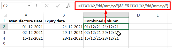
- =CONCAT(TEXT(A2,”dd/mm/yy”),”-“,TEXT(B2,”dd/mm/yy”))

In this example, A2 and B2 contain the original dates in proper date format.
How to Add Additional Text in Combined Cells?
Sometimes, you may need to add additional text in between or after the combined cells. To do this, follow the same technique you followed when you added spaces. Insert your custom text in between double quotes.
For example, if you want to add the phrase “was born on” in-between names and date of birth columns, you can use either one of these two formulas:
=CONCAT(A2,” expires on “,TEXT(B2,”dd/mm/yy”))

=TEXT(A2,”dd/mm/yy”)&”-“&TEXT(B2,”dd/mm/yy”)

How to Remove the Formula from the Combined Columns?
The combined column that you created, using the above methods is going to be dynamic. That means any change in the original values will affect the values in the combined column. To prevent this, copy the values of the combined column and paste them as values in the same column, or even a different column.
How to Merge Columns in Excel?
If you don’t want to combine the values of two columns, but want to just merge two columns into one instead, you can follow these steps:
- Select the cells or columns that you want to merge.
- Click on the “Merge & Centre” option on the “Home” tab.
Excel will merge the selected columns into one column.
Note: Please keep in mind that this will only keep the value from the upper-left corner cell and clear all other values.
Suggested Reads:
Excel Sumifs & Sumif Functions – The No.1 Complete Guide
Create An Excel Dashboard In 5 Minutes – The Best Guide
Dynamic Dropdown Lists In Excel – Top Data Validation Guide
Closing Thoughts
That’s all folks. In this guide, I have shown you how to combine two columns in Excel using the easiest methods. Try using these methods in a practice worksheet and let us know if you have any questions about it.
Want more high-quality guides for Excel? Check out our free Excel resources centre.
Click here to access in-depth Excel training courses and master in-demand advanced Excel skills.
Simon Sez IT has been teaching critical IT software for over ten years. For a low, monthly fee you can get access to 100+ IT training courses by seasoned professionals.
Simon Calder

Chris “Simon” Calder was working as a Project Manager in IT for one of Los Angeles’ most prestigious cultural institutions, LACMA.He taught himself to use Microsoft Project from a giant textbook and hated every moment of it. Online learning was in its infancy then, but he spotted an opportunity and made an online MS Project course — the rest, as they say, is history!