Join cell in excel

Microsoft Excel is the most renowned tool used all over the world to perform data collection, data management, and for analytics. It becomes one of the basic needs to understand how to apply formulas correctly while using Excel. Primarily you collect and analyze data with Excel, however today we will discuss how to join cells in Excel.

Sometimes, you can use shortcuts to collect data because it helps speed up the function. Below you will find some useful hacks that ultimately let you merge two cells in Excel. When it comes to organizing data, merging plays an important role.

Benefits of Merging Two Cells in Excel

When you merge cells in Excel, you will be able to sort out data nicely from multiple strands. You can apply this feature on both horizontal and vertical cells. Once the procedure is done, you will see all merged data in one big cell instead of many columns. It helps to make the spreadsheet presentable and uniform.

CONCATENATE Method to Join Cells

Sometimes, when you organize data, it might be possible that some part of your data is lost. You apply multiple features to maintain data properly, but you end up losing some data unintentionally. For this, you follow the CONCATENATE method to avoid data loss.

To apply this method, add =CONCATENATE(A1.” “,B1) in your dataset.

You always have to enter a space in this method and you can even use the command without a separator as well. in that case, the syntax would be: =CONCATENATE(A1, B1).

How to Join Cells in Excel?

Below you will find some useful steps to follow in order to learn how easily you can merge multiple cells in an Excel sheet.

• Choose the cells that needed to be merged. Highlight these cells with your mouse. Or else you can start from a cell by pressing and holding Shift and then the arrows to select the end.

• Click on the Format Cells button given on the Home ribbon. Or else you can press the CTRL + 1 from the keyboard and it will open up the Format Cells dialog box.

• Click on the Alignment tab given in the Format Cells menu and check the box of Merge Cells.

• Choose the center to put the title in the center and set the background color to make your title look awesome.

How to Join Cells in Excel with Shortcut?

Other than the above method, you can apply some shortcuts as well to merge multiple cells in one large cell. For this, select all the cells that needed to be merged and then enter the following shortcut keys from your keyboard.

Excel Shortcuts for Windows

Press ALT + H + M + M to merge cells.

Press ALT + H + M + C to merge and center cells.

Press ALT + H + M + A to merge across cells

Press ALT + H + M + U to unmerge cells.

Excel Shortcuts for Mac OS

You will not find an ALT key in the Apple devices that’s why you will not be able to apply the above-mentioned shortcuts on Mac OS. For this, you will have to set your own shortcut to merge cells. Here is how you can do it:

• Click the “Tools” option given under the navigation bar.
• Choose “Customize Keyboard.”
• You will see a pop-up and click on “Specify a Command” placed under the header. There are two columns: Categories and Commands. Click on the “Home” tab for Categories columns and choose “Merge Cells” for Commands.
• Now, you will see a text box placed under the “Press new keyboard shortcut” option. Enter the shortcut keys here, such as:

CONTROL + M

• Click OK.

Now the shortcut keys will be functional to merge cells.

Similarly, you can set further shortcuts to merge cells, unmerge cells, merge and center.

Merge and Center Cells

You can merge and center data by following the below-given procedure. Sometimes when you need the title of a spreadsheet document in the center, you will need to set it in the center.

• Choose the cells that needed to be merged.
• Find and click on the “Merge & Center” option from the “Home” tab.
• All the selected cells will be merged and your data will be centered.
• Bear in mind that all the data except left cell data will be removed if the content is in separate cells.

Merge Cells without Losing Data

You must be thinking about how you can merge cells without losing your data. For this, we have a highly reliable method here.

Other than CONCATENATE method, you can use the Ampersand method to merge cells without losing data. CONCATENATE method is explained above; now let’s move on to the Ampersand formula.

• Highlight all the cells in which you need to put the merged data. Type “=”.
• Choose the first cell and enter “&”.
• Make sure you have entered “ “ to keep space between the existing data.
• Now, choose the second cell and add the entire formula. Press Enter key.
• Your data is merged and you will see it in the next cell.

Press and hold the left mouse button to drag the formula down. It will get you the same outcome for further following cells.

Final Thoughts

That’s it!

Now, you can freely merge cells whenever you need. You are now fully aware of multiple methods that can help you in merging cells. Keep trying and one day you will become an expert.

EDIT: If you are using Excel 2019 or Office 365 you can use the TEXTJOIN function to solve this problem. Click here for the new article:

How to Join Text from Several Cells in Excel using TEXTJOIN

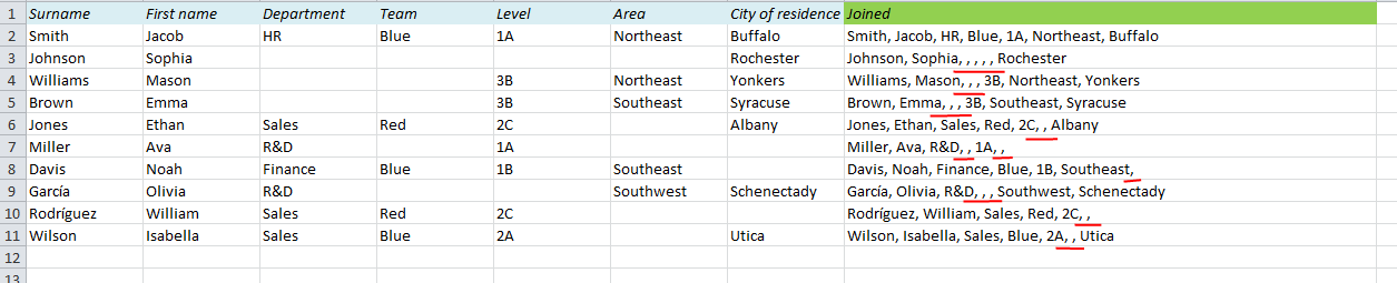
Unclean data can cause a lot of problems in Excel. In this post I will show how you can join data from different columns with a comma between them. That’s the easy part. The problem occurs when you have empty cells in your data, like in the table below. The result of the first row looks fine, but if you look at the rows with empty cells, you get too many commas:

Joining the strings

First, let’s look at how we join the strings. We’ll deal with the commas later.

There are two ways to do this, either with the CONCATENATE function, or with the Ampersand (&)operator. With Ampersand, you start with the first element, add the the “&”, type the next, add another “&”, and so on:

=A2&B2&C2&D2&E2&F2&G2

The result of this formula is “SmithJacobHRBlue1ANortheastBuffalo”, so we have to add the commas (and a space) between the cell references. The comma+space is a text string, and has to be wrapped between double quotes:

=A2&”, “&B2&”, “&C2&”, “&D2&”, “&E2&”, “&F2&”, “&G2

The second way to join cells is the CONCATENATE function. Instead of all the Ampersand symbols, you simply start with the function name, and separate the elements with a comma (or semicolon for some international Excel users):

=CONCATENATE(A2,”, “,B2,”, “,C2,”, “,D2,”, “,E2,”, “,F2,”, “,G2)

Removing the extra commas

As we saw on the picture above, this works fine as long as there are no empty cells in the raw data. However, that is rarely the case, and if we don’t want the extra commas in our result, we have to adjust our formula a little bit.

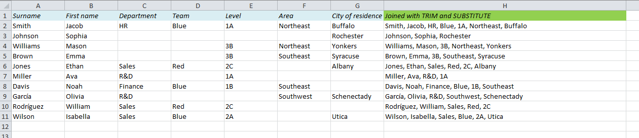
The TRIM function in Excel can be used to get rid of excess spaces in a text string. Unfortunately, there is no function that removes excess commas, so we have to start with a string with spaces instead of commas, then remove excess spaces, and finally replace the spaces with commas. Here are the 3 steps:

• Step 1: Join the cells with a space between each cell
  (The CONCATENATE part)
• Step 2: Wrap the TRIM function around it to get rid of excess spaces
• Step 3: Wrap the SUBSTITUTE function around that to replace the spaces with commas

We end up with this formula: =SUBSTITUTE(TRIM(CONCATENATE(A2,” “,B2,” “,C2,” “,D2,” “,E2,” “,F2,” “,G2)),” “,”, “)

If you are using Excel 2019 or Office 365 you can use the TEXTJOIN function to solve this problem. Click here for the new article:

How to Join Text from Several Cells in Excel using TEXTJOIN

More on text functions:

• How to Join Text from Several Cells in Excel using TEXTJOIN
• Convert text to number with formula
• Create random text strings and line breaks with the CHAR function
• Use Excel to Count Words
• Bahttext
• Use Excel to count characters

Are you using a non-English version of Excel? Click here for translations of the 140 most common functions in 17 different languages:

Catalan
Czech
Danish
Dutch
Finnish
French
Galician
German
Hungarian
Italian
Norwegian
Polish
Portuguese (Brazilian)
Portuguese (European)
Russian
Spanish
Swedish
Turkish

How to merge and center

1. Highlight the cells you want to merge and center.
2. Click on “Merge & Center,” which should be displayed in the “Alignment” section of the toolbar at the top of your screen. The top row of cells here is selected.
3. The cells will now be merged with the data centered in the merged cell.

How do you link two cells in Excel?

Combine data with the Ampersand symbol (&)

1. Select the cell where you want to put the combined data.
2. Type = and select the first cell you want to combine.
3. Type & and use quotation marks with a space enclosed.
4. Select the next cell you want to combine and press enter. An example formula might be =A2&” “&B2.

Can you join cells in Excel?

To merge a group of cells:
Highlight or select a range of cells. Right-click on the highlighted cells and select Format Cells…. Click the Alignment tab and place a checkmark in the checkbox labeled Merge cells.

How do you automatically link cells in Excel?

Go to Sheet2, click in cell A1 and click on the drop-down arrow of Paste button on the Home tab and select Paste Link button. It will generate a link by automatically entering the formula =Sheet1! A1 .

How do you link cells?

Create a link to a worksheet in the same workbook

1. Select the cell or cells where you want to create the external reference.
2. Type = (equal sign).
3. Switch to the worksheet that contains the cells that you want to link to.
4. Select the cell or cells that you want to link to and press Enter.

How do you merge cells in Excel without losing text?

How to merge cells in Excel without losing data

1. Select all the cells you want to combine.
2. Make the column wide enough to fit the contents of all cells.
3. On the Home tab, in the Editing group, click Fill > Justify.
4. Click Merge and Center or Merge Cells, depending on whether you want the merged text to be centered or not.

How do I merge cells in a table in Excel?

Merge cells

1. In the table, drag the pointer across the cells that you want to merge.
2. Click the Layout tab.
3. In the Merge group, click Merge Cells.

How do I enable merge and center in Excel?

Merge and Center Cells in Excel

1. Select the adjacent cells you want a merge.
2. On the Home button, go-to alignment group, click on merge and center cells in excel.
3. Click on merge and center cell in excel to combine the data into one cell.

How do you link cells in sheets?

Link to data in a spreadsheet

1. In Sheets, click the cell you want to add the link to.
2. Click Insert. Link.
3. In the Link box, click Select a range of cells to link.
4. Highlight the cell or range of cells you want to link to.
5. Click OK.
6. (Optional) Change the link text.
7. Click Apply.

Share a workbook in Excel for the web

1. Select File > Share > Share with People (or select Share in the top right).
2. In the Enter a name or email address box, type the email addresses of people you want to share with.

How do I link cells in the same worksheet in Excel?

Select a cell where you want to insert a hyperlink. Right-click on the cell and choose the Hyperlink option from the context menu. The Insert Hyperlink dialog window appears on the screen. Choose Place in This Document in the Link to section if your task is to link the cell to a specific location in the same workbook.

How do I merge rows in Excel without losing data?

Combine rows in Excel with Merge Cells add-in

1. Select the range of cells where you want to merge rows.
2. Go to the Ablebits Data tab > Merge group, click the Merge Cells arrow, and then click Merge Rows into One.
3. This will open the Merge Cells dialog box with the preselected settings that work fine in most cases.

How do I merge rows but not columns?

Select the range of cells containing the values you need to merge, and expand the selection to the right blank column to output the final merged values. Then click Kutools > Merge & Split > Combine Rows, Columns or Cells withut Losing Data. 2.

Can cells be merged in a table?

You can combine two or more table cells located in the same row or column into a single cell.Select the cells that you want to merge. Under Table Tools, on the Layout tab, in the Merge group, click Merge Cells.

How do I merge cells in Excel 2019?

How to merge cells

1. Highlight the cells you want to merge.
2. Click on the arrow just next to “Merge and Center.”
3. Scroll down to click on “Merge Cells”. This will merge both rows and columns into one large cell, with alignment intact.
4. This will merge the content of the upper-left cell across all highlighted cells.

Why won’t Excel let me merge cells?

Actually, there are two conditions that can cause the Merge and Center tool to be unavailable. You should check, first, to see if your worksheet is protected.If you turn off sharing (if it is on) and disable protection (if the worksheet is protected), then the tool should once again be available.

How do you unlock merge cells in Excel?

1. Unlock all cells on the sheet.

1. Press Ctrl + A or click the Select All button.
2. Press Ctrl + 1 to open the Format Cells dialog (or right-click any of the selected cells and choose Format Cells from the context menu).
3. In the Format Cells dialog, switch to the Protection tab, uncheck the Locked option, and click OK.

What is the shortcut key to merge cells in Excel?

How to Merge Cells in Excel Shortcut

1. Merge Cells: ALT H+M+M.
2. Merge & Center: ALT H+M+C.
3. Merge Across: ALT H+M+A.
4. Unmerge Cells: ALT H+M+U.

How do you reference a cell in another worksheet?

To reference a cell or range of cells in another worksheet in the same workbook, put the worksheet name followed by an exclamation mark (!) before the cell address. For example, to refer to cell A1 in Sheet2, you type Sheet2!A1. For example, to refer to cells A1:A10 in Sheet2, you type Sheet2!A1:A10.

Why do you link the spreadsheet data?

✦ Link Worksheet Data – Method Two ✦
As in the example above, we are bringing in the value of cell B6 from the Paris worksheet. The destination worksheet displays the formula value, and the link formula displays in the formula bar (figure 4).

What is a hyperlink in computer?

In a website, a hyperlink (or link) is an item like a word or button that points to another location. When you click on a link, the link will take you to the target of the link, which may be a webpage, document or other online content.