
UsedRange, as the name suggests, are the ranges that do not include the empty cells in the used ranges as some values. So in VBA, used ranges are the property of the range object for those ranges of cells in rows and columns that are not empty and have some values.
Table of contents
- UsedRange in VBA Excel
- Examples of Excel VBA UsedRange Property
- Example #1
- Example #2
- Example #3
- Example #4
- Things to Remember About VBA UsedRange
- Recommended Articles
- Examples of Excel VBA UsedRange Property
UsedRange in VBA Excel
The UsedRange in VBA is a worksheet property that returns a range object representing the range used (all Excel cells used or filled in a worksheet) on a particular worksheet. It is a property representing the area covered or bounded by the top-left used cell and the last right-used cells in a worksheet.
We can describe a ‘Used Cell’ as a cell containing any formula, formatting, value, etc. We can also select the last used cell by pressing the CTRL+END keys on the keyboard.
Following is an illustration of a UsedRange in a worksheet:
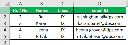
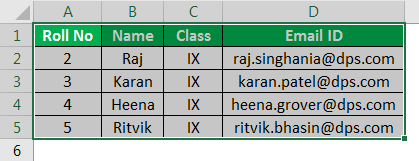
We can see in the above screenshot that the UsedRange is A1:D5.
Examples of Excel VBA UsedRange Property
Let us look at some examples below to see how we can use the UsedRange property in a worksheet to find the used range in VBARange is a property in VBA that helps specify a particular cell, a range of cells, a row, a column, or a three-dimensional range. In the context of the Excel worksheet, the VBA range object includes a single cell or multiple cells spread across various rows and columns.read more:
You can download this VBA UsedRange Excel Template here – VBA UsedRange Excel Template
Example #1
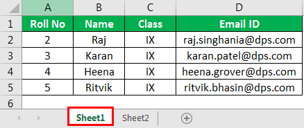
We have an Excel file containing two worksheets, and we wish to find and select the used range on Sheet1.
Let us see what the Sheet1 contains:
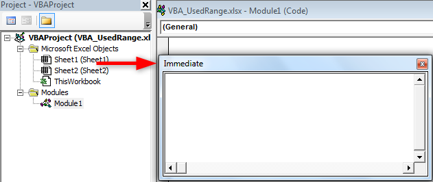
We use the UsedRange property in the VBA immediate window to accomplish this task. VBA immediate window is a tool that helps to get information about Excel files and quickly execute or debug any VBA codeVBA code refers to a set of instructions written by the user in the Visual Basic Applications programming language on a Visual Basic Editor (VBE) to perform a specific task.read more, even if the user is not writing any macros. It is located in the Visual Basic Editor and can be accessed as follows:
- Go to the Developer tab ExcelEnabling the developer tab in excel can help the user perform various functions for VBA, Macros and Add-ins like importing and exporting XML, designing forms, etc. This tab is disabled by default on excel; thus, the user needs to enable it first from the options menu.read more, click on Visual Basic Editor, or press Alt+F11 to open the Visual Basic Editor window.
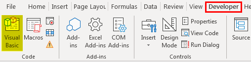
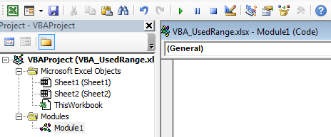
In doing this, a window opens as follows:
- Next, press Ctrl+G to open the immediate window and type the code.
The immediate window looks like this:
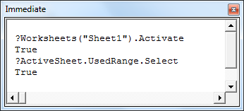
- The following code will select the used range on Sheet1.
Code:
?Worksheets("Sheet1").Activate
True
?ActiveSheet.UsedRange.Select
True
The first statement of the code will activate Sheet1 of the file, and the second statement will select the used range in that active sheet.
On writing this code, we see that the range used in Sheet1 gets selected as follows:
Example #2
In this example, we wish to find the total number of rows used in Sheet1. To do this, we follow the below steps:
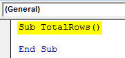
- First, create a Macro name in the module.
Code:
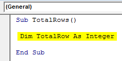
Sub TotalRows()

End Sub
- Define the variable TotalRow as an Integer in VBAIn VBA, an integer is a data type that may be assigned to any variable and used to hold integer values. In VBA, the bracket for the maximum number of integer variables that can be kept is similar to that in other languages. Using the DIM statement, any variable can be defined as an integer variable.read more:
Code:
Sub TotalRows()

 Dim TotalRow As Integer

End Sub
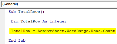
- Now, assign the variable TotalRow with the formula to calculate the total number of rows:
Code:
Sub TotalRows()

 Dim TotalRow As Integer

 TotalRow = ActiveSheet.UsedRange.Rows.Count

End Sub
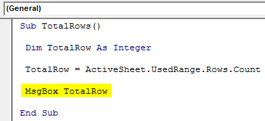
- Now, the resultant value of TotalRow can be displayed and returned using a VBA message boxVBA MsgBox function is an output function which displays the generalized message provided by the developer. This statement has no arguments and the personalized messages in this function are written under the double quotes while for the values the variable reference is provided.read more (MsgBox) as follows:
Code:
Sub TotalRows()

 Dim TotalRow As Integer

 TotalRow = ActiveSheet.UsedRange.Rows.Count

 MsgBox TotalRow

End Sub
- Now, we run this code manually or by pressing F5, and we get the total number of rows used in Sheet1 displayed in a message box as follows:
So, we can see in the above screenshot that ‘5’ is returned in the message box. As shown in Sheet1, the total number of rows in the used range is 5.
Example #3
Similarly, if we wish to find the total number of columns used in Sheet1, we will follow the same steps as above except for a slight change in the code as follows:
Code:
Sub TotalCols()

 Dim TotalCol As Integer

 TotalCol = ActiveSheet.UsedRange.Columns.Count

 MsgBox TotalCol

End Sub
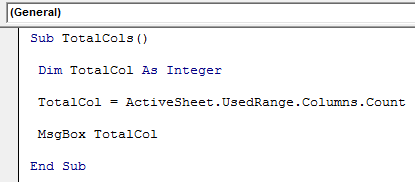
Now, when we run this code manually or by pressing F5, we get the total number of columns used in Sheet1 displayed in a message box as follows:
So, ‘4’ is returned in the message box, and as we can see in Sheet1, the total number of columns in the used range is 4.
Example #4
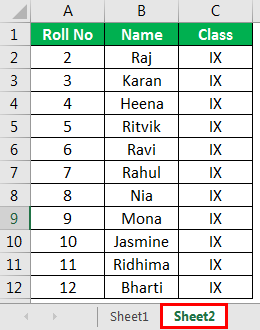
Let’s say we wish to find the last used row and column number in Sheet2 of the file. But, first, let us see what the Sheet2 contains:
To do this, we follow the below steps:
- First, create a Macro name in the module.
Code:
Sub LastRow()

End Sub

- Define the variable LastRow as Integer.
Code:
Sub LastRow()

 Dim LastRow As Integer

End Sub

- Now, assign the variable LastRow with the formula to calculate the last used row number:
Code:
Sub LastRow()

  Dim LastRow As Integer

  LastRow = ActiveSheet.UsedRange.SpecialCells(xlCellTypeLastCell).Row

End Sub
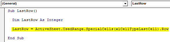
The SpecialCells Method in Excel VBA returns«GoSub» in the GoSub Return Statement signifies that it will go to the indicated line of code and complete a task until it finds the statement «Return.» It’s a lifesaver for those who know the in and out of VBA coding.read more a range object that represents only the types of cells specified. The syntax for the SpecialCells method is:
RangeObject.SpecialCells (Type, Value)
The above code, xlCellTypeLastCell: represents the last cell in the used range.
Note: ‘xlCellType’ will even include empty cells with the default format of any of their cells changed.
- Now, the resultant value of the LastRow number can be displayed and returned using a message box (MsgBox) as follows:
Code:
Sub LastRow()

 Dim LastRow As Integer

 LastRow = ActiveSheet.UsedRange.SpecialCells(xlCellTypeLastCell).Row

 MsgBox LastRow

End Sub
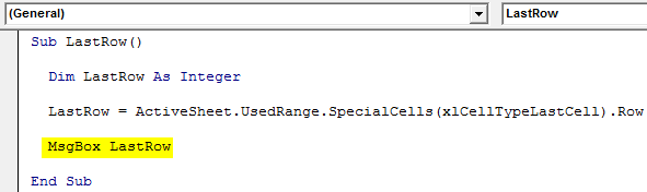
- Now, we run this code manually or by pressing F5, and we get the last used row number in Sheet2 displayed in a message box as follows:
So, we can see in the above screenshot that ‘12’ is returned in the message box. As shown in Sheet2, the last used row number is 12.
Similarly, if we wish to find the last used column number in Sheet2, we will follow the same steps as above except for a slight change in the code as follows:
Code:
Sub LastCol()

  Dim LastCol As Integer

  LastCol = ActiveSheet.UsedRange.SpecialCells(xlCellTypeLastCell).Column

  MsgBox LastCol

End Sub
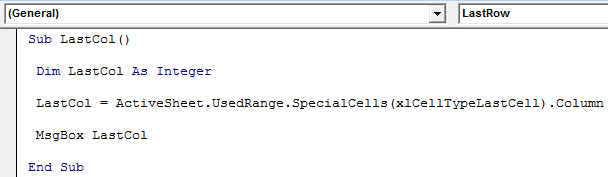
Now, when we run this code manually or by pressing F5, we get the last used column number in Sheet2 displayed in a message box as follows:
So, we can see in the above screenshot that ‘3’ is returned in the message box. As shown in Sheet2, the last used column number is 3.
Things to Remember About VBA UsedRange
- VBA UsedRange is a rectangle range.
- VBA UsedRange includes cells having any data or being formatted etc.
- Excel VBA UsedRange does not necessarily include the top-left cell of the worksheet.
- UsedRange does not necessarily consider the active cell as used.
- UsedRange can be used to find the last used row in VBAThe End(XLDown) method is the most commonly used method in VBA to find the last row, but there are other methods, such as finding the last value in VBA using the find function (XLDown).read more and to reset the used range, etc.
- Pressing the shortcut Excel keysAn Excel shortcut is a technique of performing a manual task in a quicker way.read more CTRL+SHIFT+ENTER on a keyboard can be used to extend the selection from an active cell to the last used cell on a worksheet.
Recommended Articles
This article has been a guide to VBA UsedRange. Here, we will show you how the UsedRange Property in a worksheet finds the used rows and columns in Excel VBA, practical examples, and a downloadable template. Below you can find some useful Excel VBA articles: –
- VBA Filter
- Excel VBA Activate Sheet
- VBA Val
Used Area of an Excel Sheet
There are many situations when we need to perform an action on all rows and columns with data in an Excel sheet. In order to do that, you need to know which row/column of data is the last. In other cases, we need to know the entire used area of a sheet (a combination of rows and columns with data). This area is also called a used range of an Excel sheet. This includes blank rows/columns — or even cells that are within the used range.
Selecting the Whole Used Range
To select the entire used range from a cell, SHIFT + CTRL + END keys can be pressed together after selecting a used cell.
Image of a Used Range
In this image, the highlighted areas are included in the used range though they are blank.
The areas highlighted in red are within the 13 rows and column I. Hence, those cells are included.
The cells highlighted in black were used initially though the data is now deleted. So, all columns up to the last used column and all rows up to the last used row are considered “USED.”

Selecting a Used Range by Row or by Column
SHIFT + CTRL + the arrow key (up/down/left/right) can select the used range by column/by row. But the drawback here is that this will not select the range up to the last used row/column. Instead, it will select the range until the cell just before a blank cell on its way.
For example, SHIFT + CTRL + down arrow from Cell B1 has selected the range of cells as in the image.

But repeated usage of the same keys i.e. pressing the combination of keys (SHIFT + CTRL + down arrow) several times can help in selecting the area until the last used row.

Find the Last Used Cell
To find the last used cell CTRL and END keys have to be used together. This will automatically select the cell which is the intersection of the last used row and last used column.

Used Range in VBA
It is now time to see how you can transfer this concept to VBA.
Here is a small piece of code that first selects a sheet and then highlights/selects the used range of that active sheet.
Sub usedrange_demo()
Sheets("snackbar").Select
ActiveSheet.UsedRange.Select
End Sub
Output: Same as the first image in this article.
Find the Number of Used Rows in a Sheet
This piece of code can help to find the number of rows that are in the used range of a sheet.
Sub usedrange_demo()
Dim rows
Sheets("snackbar").Select
rows = ActiveSheet.UsedRange.rows.Count
MsgBox rows
End Sub

Find the Number of Used Columns in an Active Sheet
Similar to the above code, here is another code snippet that counts the number of columns within the used range of a sheet and displays the result in a message box.
Sub usedrange_demo()
Dim cols
Sheets("snackbar").Select
cols = ActiveSheet.UsedRange.Columns.Count
MsgBox cols
End Sub

Specialcells Method in VBA
SpecialCells is a built in function offered by VBA. It returns a range object which represents only specified types of cells.
Syntax:
RangeObject.SpecialCells (<Type> , <Value>)
Using The Specialcells Function Combined with Used Range to Find the Last Row
Sub usedrange_demo1()
Dim lastrow
Sheets("snackbar").Select
lastrow = ActiveSheet.UsedRange.SpecialCells(xlCellTypeLastCell).Row
MsgBox lastrow
End Sub

Using the Specialcells Function Combined with Used Range to Find the Last Column of Date
Sub usedrange_demo1()
Dim lastcol
Sheets("snackbar").Select
lastcol = ActiveSheet.UsedRange.SpecialCells(xlCellTypeLastCell).Column
MsgBox lastcol
End Sub

Example: Calculate Simple Interest and Maturity Amount for All Rows of Data
In this program there is an Excel sheet with the principal amount, number of years, and age of the customer in different columns of the sheet. We need a program that does not use formulae. The simple interest and maturity amount should be calculated for each row but we do not know how many rows of data are there in the sheet.
| Principal amount | No of yrs | Age of customer | Simple Interest | Maturity Amount |
| 10000 | 5 | 67 | ||
| 340600 | 6 | 45 | ||
| 457800 | 8 | 34 | ||
| 23400 | 3 | 54 | ||
| 12000 | 4 | 23 | ||
| 23545 | 4 | 56 | ||
| 345243 | 2 | 55 | ||
| 34543 | 3 | 24 | ||
| 23223 | 2 | 19 | ||
| 3656 | 1 | 65 |
So, here, used range property is used to fetch the last row number. Then you can use a for loop to iterate through each row, do the calculation, and enter the result in a different column of the same row. Age is a vital information in this example, since the rate of interest is different for senior citizens.
Sub simple_interest_calculation_rows()
' declare all required variables
Dim Prin, no_of_years, cut_age, roi, simple_interest, mat_amt, lastrow
' find the last row of usedrange
lastrow = ActiveSheet.UsedRange.SpecialCells(xlCellTypeLastCell).Row
' iterate through each row in the used range
For i = 2 To lastrow
Prin = Cells(i, 1).Value
no_of_years = Cells(i, 2).Value
cut_age = Cells(i, 3).Value
' Set rate of interest depending on the cut_age of the customer ( varies for senior citizens )
If cut_age &amp;amp;gt; 59 Then
' senior citizens
roi = 10
Else
' non- senior citizens
roi = 8
End If
' Calculate the simple interest and maturity amount
simple_interest = (Prin * no_of_years * roi) / 100
mat_amt = simple_interest + Prin
' Display the calculated output
Cells(i, 4).Value = "The interest amount is " &amp;amp;amp; simple_interest
Cells(i, 5).Value = "The maturity amount is " &amp;amp;amp; mat_amt
Next
End Sub
Output of the Program:
| Principal amount | No of yrs | Age of customer | Simple Interest | Maturity Amount |
| 10000 | 5 | 67 | The interest amount is 5000 | The maturity amount is 15000 |
| 340600 | 6 | 45 | The interest amount is 163488 | The maturity amount is 504088 |
| 457800 | 8 | 34 | The interest amount is 292992 | The maturity amount is 750792 |
| 23400 | 3 | 54 | The interest amount is 5616 | The maturity amount is 29016 |
| 12000 | 4 | 23 | The interest amount is 3840 | The maturity amount is 15840 |
| 23545 | 4 | 56 | The interest amount is 7534.4 | The maturity amount is 31079.4 |
| 345243 | 2 | 55 | The interest amount is 55238.88 | The maturity amount is 400481.88 |
| 34543 | 3 | 24 | The interest amount is 8290.32 | The maturity amount is 42833.32 |
| 23223 | 2 | 19 | The interest amount is 3715.68 | The maturity amount is 26938.68 |
| 3656 | 1 | 65 | The interest amount is 365.6 | The maturity amount is 4021.6 |
Conclusion:
Some Points to Remember About the UsedRange in VBA.
- UsedRange is the used area of an Excel sheet.
- VBA UsedRange includes all cells that currently have data or some formatting .(colors/borders/shading)/earlier had data/cell format.
- The last row/column of data or the number of columns/rows in a used range of a sheet can be found using the UsedRange property in VBA.
- It is not mandatory that the top left cell be a part of the defined UsedRange.
- Selected cells are active cells and are not used cells unless they contain/contained some data/formatting.
Tagged with: Columns, documentation, Excel, Functions, Rows, specialcells, Used Range, UsedRange, VBA, VBA For Excel, VBA UsedRange
Home / VBA / How to use UsedRange Property in VBA in Excel
In VBA, the UsedRange property represents the range in a worksheet that has data in it. The usedrange starts from the first cell in the worksheet where you have value to the last cell where you have value. Just like the following example where you have used range from A1 to C11.

Note: UsedRange property is a read-only property.
Write a Code with UsedRange
Use the following code.
- First, you need to specify the worksheet.
- Then enter a dot (.) and enter “UsedRange”.
- After that, use the property or method that you want to use.
- In the end, run the code.
Sub vba_used_range()
    ActiveSheet.UsedRange.Clear
End Sub
The above code clears everything from the used range from the active sheet.
Copy UsedRange
Use the following code to copy the entire UsedRange.

Sub vba_used_range()

    ActiveSheet.UsedRange.Copy

End Sub
Count Rows and Columns in the UsedRange
There’s a count property that you can use to count rows and columns from the used range.
MsgBox ActiveSheet.UsedRange.Rows.Count
MsgBox ActiveSheet.UsedRange.Columns.Count
The above two lines of code shows a message box with the count of rows and columns that you have in the used range.
Activate the Last Cell from the UsedRange
You can also activate the last cell from the used range (that would be the last used cell in the worksheet). Consider the following code.

Sub vba_used_range()

Dim iCol As Long
Dim iRow As Long

iRow = ActiveSheet.UsedRange.Rows.Count
iCol = ActiveSheet.UsedRange.Columns.Count

ActiveSheet.UsedRange.Select
Selection.Cells(iRow, iCol).Select

End Sub
This code takes the rows and columns count using the UsedRange property and then use those counts to select the last cell from the used range.
Refer to UsedRange in a Different Worksheet
If you are trying to refer to the used range in a worksheet other than the active sheet then VBA will show an error like the following.

So, the worksheet where you are referring must be activated (only then you can use the UsedRange property).
Sub vba_used_range()

    Worksheets("Sheet4").Activate
    Worksheets("Sheet4").UsedRange.Select

End Sub
That means you can’t refer to the used range in a workbook that is closed. But you can use open a workbook first and then, activate the worksheet to use the UsedRange property.
Get the Address of the UsedRange
Use the following line of code to get the address of the used range.
Sub vba_used_range()

 MsgBox ActiveSheet.UsedRange.Address

End Sub
Count Empty Cells from the Used Range
The following code uses the FOR LOOPS (For Each) and loops through all the cells in the used range and counts cells that are empty.
Sub vba_used_range()

Dim iCell As Range
Dim iRange As Range
Dim c As Long
Dim i As Long

Set iRange = ActiveSheet.UsedRange

For Each iCell In ActiveSheet.UsedRange

    c = c + 1

    If IsEmpty(iCell) = True Then
        i = i + 1
    End If

Next iCell

MsgBox "There are total " & c & _
" cell(s) in the range, and out of those " & _
i & " cell(s) are empty."

End Sub
When you run this code, it shows a message box with the total count of cells and how many cells are empty out of that.
More Tutorials
- Count Rows using VBA in Excel
- Excel VBA Font (Color, Size, Type, and Bold)
- Excel VBA Hide and Unhide a Column or a Row
- Excel VBA Range – Working with Range and Cells in VBA
- Apply Borders on a Cell using VBA in Excel
- Find Last Row, Column, and Cell using VBA in Excel
- Insert a Row using VBA in Excel
- Merge Cells in Excel using a VBA Code
- Select a Range/Cell using VBA in Excel
- SELECT ALL the Cells in a Worksheet using a VBA Code
- ActiveCell in VBA in Excel
- Special Cells Method in VBA in Excel
- VBA AutoFit (Rows, Column, or the Entire Worksheet)
- VBA ClearContents (from a Cell, Range, or Entire Worksheet)
- VBA Copy Range to Another Sheet + Workbook
- VBA Enter Value in a Cell (Set, Get and Change)
- VBA Insert Column (Single and Multiple)
- VBA Named Range | (Static + from Selection + Dynamic)
- VBA Range Offset
- VBA Sort Range | (Descending, Multiple Columns, Sort Orientation
- VBA Wrap Text (Cell, Range, and Entire Worksheet)
- VBA Check IF a Cell is Empty + Multiple Cells
⇠ Back to What is VBA in Excel
Helpful Links – Developer Tab – Visual Basic Editor – Run a Macro – Personal Macro Workbook – Excel Macro Recorder – VBA Interview Questions – VBA Codes
|
Serge Пользователь Сообщений: 11308 |
Всем привет. Записываю макрос создания сводной: Sub Макрос1() ‘ Что не нравится? То что диапазон задаётся абсолютный «Лист1!R1C1:R2C2», но в следующий раз диапазон будет другим. Да и лист может по другому называться. Как сделать, что бы макрос сам определял кол-во заполненных строк и столбцов АКТИВНОГО листа и использовал их при создании сводной? Кроме того, сводная, по умолчанию, создаётся с названием «СводнаяТаблица1», но если сводная с таким названием уже есть в этом файле, то макрос выдаст ошибку. Как этого избежать? ЗЫ На самом деле важен только первый пункт, второй — это исключение из правил |

|
Юрий М  Модератор Сообщений: 60581 Контакты см. в профиле |
Может именованный (динамический) использовать? |
|
flash Пользователь Сообщений: 13 |
может так Range(«A1»).CurrentRegion.Address он же [A1].CurrentRegion.Address |
|
Серёг, а может примерчик выложишь в Excel’e ? А мы поиграемся |
|
|
Serge Пользователь Сообщений: 11308 |
{quote}{login=Юрий М}{date=16.11.2011 11:37}{thema=}{post}Может именованный (динамический) использовать?{/post}{/quote}Не, как это формулами сделать, я знаю. |
|
Serge Пользователь Сообщений: 11308 |
{quote}{login=}{date=16.11.2011 11:40}{thema=}{post}Серёг, а может примерчик выложишь в Excel’e ? А мы поиграемся{/post}{/quote}А какой пример? |

|
Serge Пользователь Сообщений: 11308 |
{quote}{login=Flash}{date=16.11.2011 11:39}{thema=}{post}может так Range(«A1»).CurrentRegion.Address он же [A1].CurrentRegion.Address{/post}{/quote} |
|
Serge Пользователь Сообщений: 11308 |
{quote}{login=}{date=16.11.2011 11:40}{thema=}{post}Серёг, а может примерчик выложишь в Excel’e ? А мы поиграемся{/post}{/quote}Паш, ты что-ли опять? |
|
Сводная всегда создаётся на основе каких-то данных. Конечно, эти данные могут начинаться и с C50, а не с А1. Это уже тонкости в которые мы вдаваться не будем, т.к. у вас вопросы по другой теме. Нам нужен пример ваших данных, на основе которых вы создаёте Сводную. Мы тоже хотим макросом попробовать создать сводную и посмотреть, что у нас получится и если получится дать ответ на форум. P.S. [A1].CurrentRegion.Address сувать в SourceData, только ещё название листа надо подставить |
|
|
эх, я, Серёг, я ) Я тут уже в своих никах запутался, поэтому иногда вообще ничего не пушу )) |
|
|
Kuzmich Пользователь Сообщений: 7998 |
Dim WSD As Worksheet ‘ Задать диапазон исходных данных и создать |

|
Serge Пользователь Сообщений: 11308 |
{quote}{login=}{date=16.11.2011 11:49}{thema=}{post}Сводная всегда создаётся на основе каких-то данных.{/post}{/quote}Ага. И эти данные (и их расположение)заранее не известны. |
|
Юрий М Модератор Сообщений: 60581 Контакты см. в профиле |
{quote}{login=Serge 007}{date=16.11.2011 11:41}{thema=Re: }{post}{quote}{login=Юрий М}{date=16.11.2011 11:37}{thema=}{post}Может именованный (динамический) использовать?{/post}{/quote}Не, как это формулами сделать, я знаю. Интересно именно на ВБА.{/post}{/quote}А где я говорил, что формулами? |
|
Serge Пользователь Сообщений: 11308 |
{quote}{login=хто-то}{date=16.11.2011 11:51}{thema=}{post} |
|
Serge Пользователь Сообщений: 11308 |
{quote}{login=Юрий М}{date=17.11.2011 12:02}{thema=Re: Re: }{post}А где я говорил, что формулами?{/post}{/quote}А что, можно динамический диапазон на ВБА? |
|
Serge Пользователь Сообщений: 11308 |
{quote}{login=Kuzmich}{date=16.11.2011 11:59}{thema=Re}{post}Dim WSD As Worksheet ‘ Задать диапазон исходных данных и создать |
|
Kuzmich Пользователь Сообщений: 7998 |
Это кусочек макроса, |
|
А так Activesheet.UsedRange.Address — это адрес заполненного диапазона ) Мимо не промахнётся )) |
|
|
Serge Пользователь Сообщений: 11308 |
{quote}{login=Kuzmich}{date=17.11.2011 12:10}{thema=Re}{post}Это кусочек макроса, |
|
Серёг, нельзя написать макрос, не видя структуру таблицы. Либо обходиться общими путями, как я уже писал Activesheet.UsedRange.Address |
|
|
Либо искать его границы, например, так Последний заполненный столбец в 1-ой строке FinalCol = Cells(1, Columns.Count).End(xlToLeft).Column последняя заполненная строка в 1-м столбце iLastRow = Cells(Rows.Count, «A»).End(xlUp).Row |
|
|
Serge Пользователь Сообщений: 11308 |
{quote}{login=хто-то}{date=17.11.2011 12:15}{thema=}{post}Серёг, нельзя написать макрос, не видя структуру таблицы.{/post}{/quote}Паш, ну нет этой структуры… Формулами это просто, но надо именно макросом… |
|
Кстати, могу выложить книгу в PDF формате, Создание сводных таблиц с помощью VBA.pdf http://webfile.ru/5673436 |
|
|
Kuzmich Пользователь Сообщений: 7998 |
Пример из книги Билла Джелена |
|
Юрий М Модератор Сообщений: 60581 Контакты см. в профиле |
Серж, я не спец. по сводным, но вот я о чём — у тебя в коде указываются конкретные ячейки диапазона: |
|
Serge Пользователь Сообщений: 11308 |
Сегодня я уже пас, завтра отвечу. |
|
KuklP Пользователь Сообщений: 14868 E-mail и реквизиты в профиле. |
Серег, мы с Алексом на твоем форуме выкладываи в «Файл распух…»: Я сам — дурнее всякого примера! … |
|
Serge Пользователь Сообщений: 11308 |
Спасибо, попробую разобраться. |
|
Serge Пользователь Сообщений: 11308 |
Только что получил решение. На первый взгляд то что нужно. http://www.excelworld.ru/forum/2-1005-1#11188 |
|
ZVI  Пользователь Сообщений: 4328 |
#30 17.11.2011 11:59:14 Еще такой вариант: Sub CreatePT() Dim PT As PivotTable, Rng As Range, Sh As Worksheet, UsedRng As Range ‘ Задать лист, на котором предполагется создать сводную ‘ Удалить все сводные с листа (для примера) ‘ Определить диапазон используемых ячеек листа полсле удаления сводных ‘ Задать динамический диапазон ячеек, примыкающих к первой ячейке данных ‘ Проверить, что не промахнулись ‘ Создать новую таблицу правее диапазона на 1 столбец ‘ Активировать 1-ю ячейку созданной сводной таблицы ‘ Сообщить End Sub |
Присвоение диапазона ячеек объектной переменной в VBA Excel. Адресация ячеек в переменной диапазона и работа с ними. Определение размера диапазона. Примеры.
Присвоение диапазона ячеек переменной
Чтобы переменной присвоить диапазон ячеек, она должна быть объявлена как Variant, Object или Range:
|
Dim myRange1 As Variant Dim myRange2 As Object Dim myRange3 As Range |
Чтобы было понятнее, для чего переменная создана, объявляйте ее как Range.
Присваивается переменной диапазон ячеек с помощью оператора Set:
|
Set myRange1 = Range(«B5:E16») Set myRange2 = Range(Cells(3, 4), Cells(26, 18)) Set myRange3 = Selection |
В выражении Range(Cells(3, 4), Cells(26, 18)) вместо чисел можно использовать переменные.
Для присвоения диапазона ячеек переменной можно использовать встроенное диалоговое окно Application.InputBox, которое позволяет выбрать диапазон на рабочем листе для дальнейшей работы с ним.
Адресация ячеек в диапазоне
К ячейкам присвоенного диапазона можно обращаться по их индексам, а также по индексам строк и столбцов, на пересечении которых они находятся.
Индексация ячеек в присвоенном диапазоне осуществляется слева направо и сверху вниз, например, для диапазона размерностью 5х5:
| 1 | 2 | 3 | 4 | 5 |
| 6 | 7 | 8 | 9 | 10 |
| 11 | 12 | 13 | 14 | 15 |
| 16 | 17 | 18 | 19 | 20 |
| 21 | 22 | 23 | 24 | 25 |
Индексация строк и столбцов начинается с левой верхней ячейки. В диапазоне этого примера содержится 5 строк и 5 столбцов. На пересечении 2 строки и 4 столбца находится ячейка с индексом 9. Обратиться к ней можно так:
|
‘обращение по индексам строки и столбца myRange.Cells(2, 4) ‘обращение по индексу ячейки myRange.Cells(9) |
Обращаться в переменной диапазона можно не только к отдельным ячейкам, но и к части диапазона (поддиапазону), присвоенного переменной, например,
обращение к первой строке присвоенного диапазона размерностью 5х5:
|
myRange.Range(«A1:E1») ‘или myRange.Range(Cells(1, 1), Cells(1, 5)) |
и обращение к первому столбцу присвоенного диапазона размерностью 5х5:
|
myRange.Range(«A1:A5») ‘или myRange.Range(Cells(1, 1), Cells(5, 1)) |
Работа с диапазоном в переменной
Работать с диапазоном в переменной можно точно также, как и с диапазоном на рабочем листе. Все свойства и методы объекта Range действительны и для диапазона, присвоенного переменной. При обращении к ячейке без указания свойства по умолчанию возвращается ее значение. Строки
|
MsgBox myRange.Cells(6) MsgBox myRange.Cells(6).Value |
равнозначны. В обоих случаях информационное сообщение MsgBox выведет значение ячейки с индексом 6.
Важно: если вы планируете работать только со значениями, используйте переменные массивов, код в них работает значительно быстрее.
Преимущество работы с диапазоном ячеек в объектной переменной заключается в том, что все изменения, внесенные в переменной, применяются к диапазону (который присвоен переменной) на рабочем листе.
Пример 1 — работа со значениями
Скопируйте процедуру в программный модуль и запустите ее выполнение.
|
1 2 3 4 5 6 7 8 9 10 11 12 13 14 15 16 17 18 19 20 21 22 23 24 25 |
Sub Test1() ‘Объявляем переменную Dim myRange As Range ‘Присваиваем диапазон ячеек Set myRange = Range(«C6:E8») ‘Заполняем первую строку ‘Присваиваем значение первой ячейке myRange.Cells(1, 1) = 5 ‘Присваиваем значение второй ячейке myRange.Cells(1, 2) = 10 ‘Присваиваем третьей ячейке ‘значение выражения myRange.Cells(1, 3) = myRange.Cells(1, 1) _ * myRange.Cells(1, 2) ‘Заполняем вторую строку myRange.Cells(2, 1) = 20 myRange.Cells(2, 2) = 25 myRange.Cells(2, 3) = myRange.Cells(2, 1) _ + myRange.Cells(2, 2) ‘Заполняем третью строку myRange.Cells(3, 1) = «VBA» myRange.Cells(3, 2) = «Excel» myRange.Cells(3, 3) = myRange.Cells(3, 1) _ & » « & myRange.Cells(3, 2) End Sub |
Обратите внимание, что ячейки диапазона на рабочем листе заполнились так же, как и ячейки в переменной диапазона, что доказывает их непосредственную связь между собой.
Пример 2 — работа с форматами
Продолжаем работу с тем же диапазоном рабочего листа «C6:E8»:
|
Sub Test2() ‘Объявляем переменную Dim myRange As Range ‘Присваиваем диапазон ячеек Set myRange = Range(«C6:E8») ‘Первую строку выделяем жирным шрифтом myRange.Range(«A1:C1»).Font.Bold = True ‘Вторую строку выделяем фоном myRange.Range(«A2:C2»).Interior.Color = vbGreen ‘Третьей строке добавляем границы myRange.Range(«A3:C3»).Borders.LineStyle = True End Sub |
Опять же, обратите внимание, что все изменения форматов в присвоенном диапазоне отобразились на рабочем листе, несмотря на то, что мы непосредственно с ячейками рабочего листа не работали.
Пример 3 — копирование и вставка диапазона из переменной
Значения ячеек диапазона, присвоенного переменной, передаются в другой диапазон рабочего листа с помощью оператора присваивания.
Скопировать и вставить диапазон полностью со значениями и форматами можно при помощи метода Copy, указав место вставки (ячейку) на рабочем листе.
В примере используется тот же диапазон, что и в первых двух, так как он уже заполнен значениями и форматами.
|
1 2 3 4 5 6 7 8 9 10 11 12 13 14 15 16 17 18 |
Sub Test3() ‘Объявляем переменную Dim myRange As Range ‘Присваиваем диапазон ячеек Set myRange = Range(«C6:E8») ‘Присваиваем ячейкам рабочего листа ‘значения ячеек переменной диапазона Range(«A1:C3») = myRange.Value MsgBox «Пауза» ‘Копирование диапазона переменной ‘и вставка его на рабочий лист ‘с указанием начальной ячейки myRange.Copy Range(«E1») MsgBox «Пауза» ‘Копируем и вставляем часть ‘диапазона из переменной myRange.Range(«A2:C2»).Copy Range(«E11») End Sub |
Информационное окно MsgBox добавлено, чтобы вы могли увидеть работу процедуры поэтапно, если решите проверить ее в своей книге Excel.
Размер диапазона в переменной
При получении диапазона с помощью метода Application.InputBox и присвоении его переменной диапазона, бывает полезно узнать его размерность. Это можно сделать следующим образом:
|
Sub Test4() ‘Объявляем переменную Dim myRange As Range ‘Присваиваем диапазон ячеек Set myRange = Application.InputBox(«Выберите диапазон ячеек:», , , , , , , 8) ‘Узнаем количество строк и столбцов MsgBox «Количество строк = « & myRange.Rows.Count _ & vbNewLine & «Количество столбцов = « & myRange.Columns.Count End Sub |
Запустите процедуру, выберите на рабочем листе Excel любой диапазон и нажмите кнопку «OK». Информационное сообщение выведет количество строк и столбцов в диапазоне, присвоенном переменной myRange.