Is unique function in excel

The UNIQUE function returns a list of unique values in a list or range. 

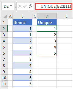
Return unique values from a list of values

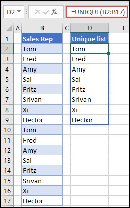
Return unique names from a list of names

=UNIQUE(array,[by_col],[exactly_once])

The UNIQUE function has the following arguments:

Argument	Description
array Required	The range or array from which to return unique rows or columns
[by_col] Optional	The by_col argument is a logical value indicating how to compare. TRUE will compare columns against each other and return the unique columns FALSE (or omitted) will compare rows against each other and return the unique rows
[exactly_once] Optional	The exactly_once argument is a logical value that will return rows or columns that occur exactly once in the range or array. This is the database concept of unique. TRUE will return all distinct rows or columns that occur exactly once from the range or array FALSE (or omitted) will return all distinct rows or columns from the range or array

Notes: 

• An array can be thought of as a row or column of values, or a combination of rows and columns of values. In the examples above, the arrays for our UNIQUE formulas are range D2:D11, and D2:D17 respectively.

• The UNIQUE function will return an array, which will spill if it’s the final result of a formula. This means that Excel will dynamically create the appropriate sized array range when you press ENTER. If your supporting data is in an Excel Table, then the array will automatically resize as you add or remove data from your array range if you’re using Structured References. For more details, see this article on Spilled Array Behavior.

• Excel has limited support for dynamic arrays between workbooks, and this scenario is only supported when both workbooks are open. If you close the source workbook, any linked dynamic array formulas will return a #REF! error when they are refreshed.

Examples

Example 1

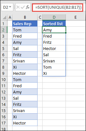
This example uses SORT and UNIQUE together to return a unique list of names in ascending order.

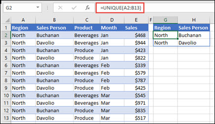
Example 2

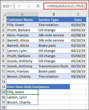
This example has the exactly_once argument set to TRUE, and the function returns only those customers who have had service one time. This can be useful if you want to identify people who have not returned for additional service, so you can contact them.

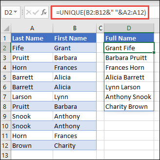
Example 3

This example uses the ampersand (&) to concatenate last name and first name into a full name. Note that the formula references the entire range of names in A2:A12 and B2:B12. This allows Excel to return an array of all names.

Tips: 

• If you format the range of names as an Excel table, then the formula will automatically update when you add or remove names.

• If you want to sort the list of names, you can add the SORT function: =SORT(UNIQUE(B2:B12&» «&A2:A12))

Example 4

This example compares two columns and returns only the unique values between them.

Need more help?

You can always ask an expert in the Excel Tech Community or get support in the Answers community.

See Also

FILTER function

RANDARRAY function

SEQUENCE function

SORT function

SORTBY function

#SPILL! errors in Excel

Dynamic arrays and spilled array behavior

Implicit intersection operator: @

I can’t even begin to count the number of times I have created a unique list in Excel. I have performed it manually using remove duplicates from the ribbon, using PivotTables and with complex formulas, but that is now a thing of the past. When Microsoft announced changes to Excel’s calculation engine in September 2018, they also announced a host of new functions, one of which was the UNIQUE function in Excel.

At the time of writing, the UNIQUE function is only available for Microsoft 365, Excel Online and Excel 2021. It will not be available in Excel 2019 or earlier versions.

Download the example file: Click the link below to download the example file used for this post:

Watch the video:

Watch the video on YouTube

The arguments of the UNIQUE function

The UNIQUE function is straightforward to apply, as shown by the animation below.

UNIQUE has just three arguments. The last two are optional arguments and quite obscure, so you will only use them occasionally.

=UNIQUE(array, [by_col], [exactly_once])

• array: the range or array to return values from.
• [by_col]: an optional argument where:
  • FALSE = compare by row
  • TRUE = compare by column.
  If excluded, the argument defaults to FALSE. The impact of this is demonstrated in Example 4.
• [exactly_once]: This argument depends on your interpretation of the word unique. If you want a list that includes only the items that appear once, then use TRUE for this argument. If you want a list that contains one instance of each item (i.e., a distinct list), then use FALSE. This is an optional argument and if excluded, will default to FALSE. The impact of this is demonstrated in Example 1.

Examples of using the UNIQUE function

The following examples illustrate how to use the UNIQUE function in Excel.

Example 1 – The difference between unique and distinct

The last argument of the UNIQUE function determines if it returns a distinct or unique list.

Distinct list

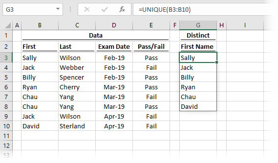
The formula in cell C3 is:

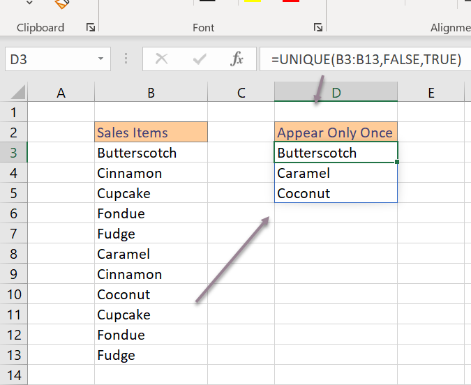
=UNIQUE(B3:B10)

As the third argument has not been used, exactly_once has defaulted to FALSE and therefore shows a list of distinct results. Sally, Jack, Billy, Ryan, Chau and David all appear in cells B3-B10; therefore, we get a list of all those names.

Unique list (exactly once)

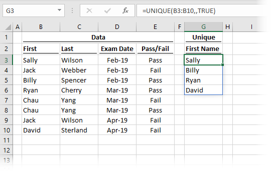
The formula in cell G3 is:

=UNIQUE(B3:B10,,TRUE)

The third argument is TRUE, therefore UNIQUE return the results which appear only once in the array. Sally, Billy, Ryan, and David all appear only once within cells B3-B10. Jack and Chau appear twice and are therefore excluded from the result.

The difference between distinct and unique lists

When using the exactly_once argument, this is an important difference to understand:

• FALSE or empty = a distinct list
• TRUE = a list of items occurring only once

My guess is that in most situations, we will be using the distinct version of UNIQUE, which is the default option anyway.

Example 2 – UNIQUE linked to an Excel table

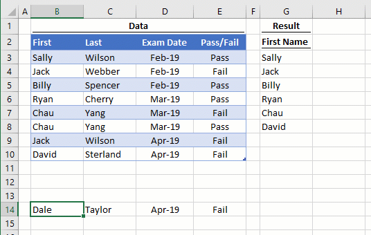
Example 2 shows how UNIQUE responds when linked to an Excel table. When a new record is added, UNIQUE automatically expands to include the additional value in the spill range. Notice that the spill range of the UNIQUE function updates as soon as new items are added to the table.

The formula in cell G3 is:

=UNIQUE(tblExam[First])

As the UNIQUE function is referencing the entire column, when the column expands or retracts, so does the result of the formula.

Example 3 – UNIQUE across multiple columns

UNIQUE is not restricted to a single column, it can assess the unique combination of multiple columns.

Method 1

This returns the unique list and retains the same number of columns as included in the first argument.

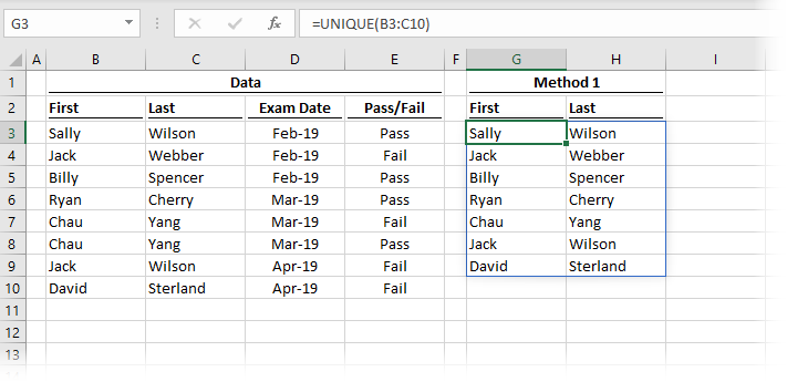
The formula in cell G3 is:

=UNIQUE(B3:C10)

This includes the First and Last name columns in the array and returns both in the result. One instance of Chau Yang has been excluded as it appears twice in the source data.

Method 2

The second method uses functionality from the new calculation engine to concatenate columns before applying the UNIQUE function. As a result, only a single column of values is returned.

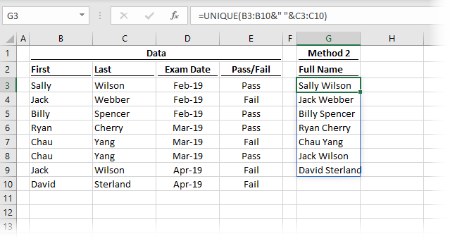
The formula in cell G3 is:

=UNIQUE(B3:B10&" "&C3:C10)

Again, one instance of Chau Yang has been removed to provide a unique list within a single column.

Method 3

Sometimes we want a unique list with two columns that are not next to each other. In this circumstance, we can use the CHOOSE or CHOOSECOLS (only available in Excel 365) functions to reorder the columns.

The example below uses the CHOOSE function and is available in Excel 2021 and Excel 365.

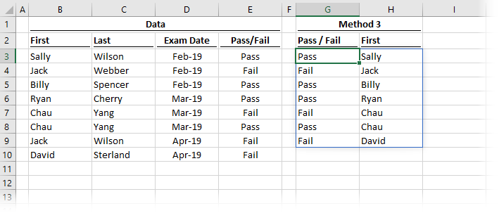
The formula in cell G3 is:

=UNIQUE(CHOOSE({1,2},E3:E10,B3:B10))

By using CHOOSE, we have defined the first array as E3-E10 and the second array as B3-B10. These are the ranges that have been returned within the spill range.

If we have Excel 365 we could use either of the following alternative formulas which use CHOOSECOLS to achieve the same result:

=CHOOSECOLS(UNIQUE(B3:E10),4,1)

=CHOOSECOLS(UNIQUE(B3:E10),{4,1})

Example 4 – Using UNIQUE across columns

By default, Excel assumes UNIQUE should be applied on a vertical list. However, it can also work on a horizontal list.

Horizontal list

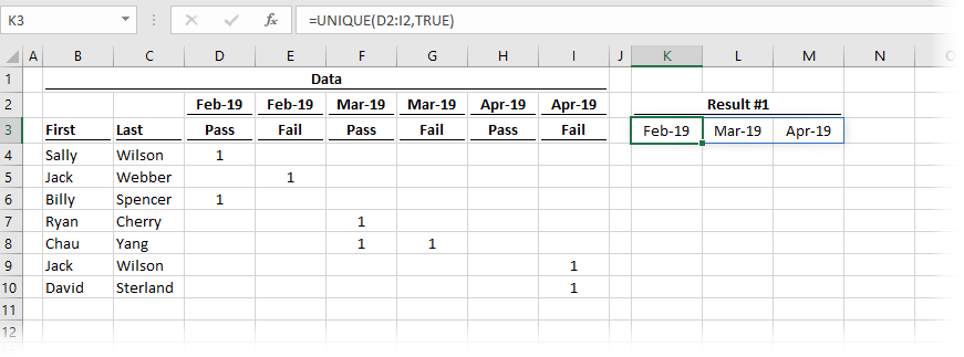
In the example above, cell K3 contains the following formula.

=UNIQUE(D2:I2,TRUE)

The second argument in UNIQUE of [by_col] is set to TRUE. This tells the function that the data is in a horizontal format.

Use TRANSPOSE to convert horizontal & vertical (and vice versa)

If we had a vertical or horizontal list that we wanted to flip, we could use the TRANSPOSE function.

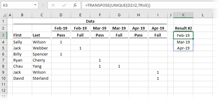
The formula in cell K3 is:

=TRANSPOSE(UNIQUE(D2:I2,TRUE))

TRANSPOSE is used to change our horizontal UNIQUE list so the output is vertical.

Example 5 – Combining UNIQUE with SORT in a data validation list

Example 5 demonstrates how to combine the UNIQUE and SORT functions together.

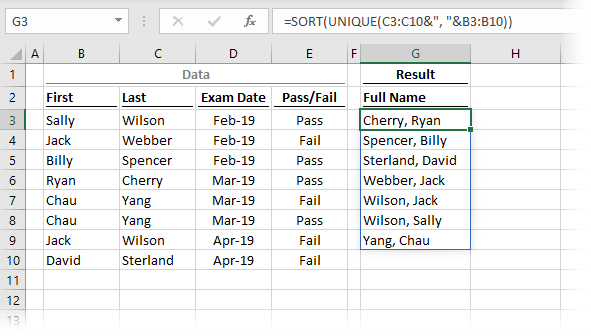
The formula in cell G3 is:

=SORT(UNIQUE(C3:C10&", "&B3:B10))

The formula returns an alphabetically sorted unique list based on the Last and First names combined.

Often the purpose of a unique sorted list is for use within a data validation drop-down list. To do this, we can use the # symbol after the cell reference to refer to the entire spill range.

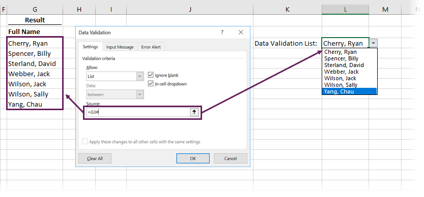
In the screenshot above, the formula is contained in cell G3. Therefore =G3# is used as the source for a data validation list. When the spill range increases or decreases in size, so does the drop-down list. It’s like magic!

Example 6 – Simple formula based Pivot Report

As a final example, we can create a simple Pivot Report using UNIQUE combined with some other common functions.

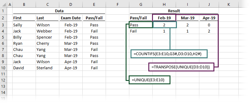
The formula in cell G3 is:

=UNIQUE(E3:E10)

This is the standard UNIQUE function applied to the Pass/Fail column.

The formula in cell H2 is:

=TRANSPOSE(UNIQUE(D3:D10))

TRANSPOSE switches the output of UNIQUE from displaying in rows to displaying in columns. The 3 distinct dates in the Exam Date column are now listed as column headers.

The formula in H3 is:

=COUNTIFS(E3:E10,G3#,D3:D10,H2#)

The COUNTIFS function includes the # references, so it automatically spills in the same way as the cells it is dependent upon.

With these 3 simple formulas, we have created a complete report – amazing! Remember, if the source is an Excel table, the output will expand as new data is added – even more amazing!!

Want to learn more?

There is a lot to learn about dynamic arrays and the new functions. Check out our other posts here to learn more:

• Introduction to dynamic arrays – learn how the excel calculation engine has changed.
• UNIQUE – to list the unique values in a range
• SORT – to sort the values in a range
• SORTBY – to sort values based on the order of other values
• FILTER – to return only the values which meet specific criteria
• SEQUENCE – to return a sequence of numbers
• RANDARRAY – to return an array of random numbers
• Using dynamic arrays with other Excel features – learn to use dynamic arrays with charts, PivotTables, pictures etc.
• Advanced dynamic array formula techniques – learn the advanced techniques for managing dynamic arrays

The Excel UNIQUE function extracts a list of unique values from a range or array. The result is a dynamic array of unique values. If this array is the final result (i.e. not handed off to another function), array values will «spill» onto the worksheet into a range that automatically updates when new uniques values are added or removed from the source range.

The UNIQUE function takes three arguments: array, by_col, and exactly_once. The first argument, array, is the array or range from which to extract unique values. This is the only required argument. The second argument, by_col, controls whether UNIQUE will extract unique values by rows or by columns. By default, UNIQUE will extract unique values in rows. To force UNIQUE to extract unique values by columns, set by_col to TRUE or 1. The last argument, exactly_once, sets behavior for values that appear more than once. By default, UNIQUE will extract all unique values, regardless of how many times they appear in array. To extract unique values that appear only once in array, set exactly_once to TRUE or 1.

Note: the UNIQUE function is not case-sensitive. UNIQUE will treat «APPLE», «Apple», and «apple» as the same text.

Basic example

The UNIQUE function extracts unique values from a range or array:

=UNIQUE({"A";"B";"C";"A";"B"}) // returns {"A";"B";"C"}

To return unique values from in the range A1:A10, you can use a formula like this:

=UNIQUE(A1:A10)

By column

By default, UNIQUE will extract unique values in rows:

=UNIQUE({1;1;2;2;3}) // returns {1;2;3}

UNIQUE will not handle the same values organized in columns:

=UNIQUE({1,1,2,2,3}) // returns {1,1,2,2,3}

To handle the horizontal array above, set the set the by_col argument to TRUE or 1:

=UNIQUE({1,1,2,2,3},1) // returns {1,2,3}

To return unique values from the horizontal range A1:E1, set the by_col argument to TRUE or 1:

=UNIQUE(A1:E1,1) // extract unique from horizontal array

Exactly once

The UNIQUE function has an optional argument called exactly_once that controls how the function deals with repeating values. By default, exactly_once is FALSE. This means UNIQUE will extract unique values regardless of how many times they appear in the source data:

=UNIQUE({1;1;2;2;3}) // returns {1;2;3}

Set exactly_once to TRUE or 1 to extract unique values that appear just once in the source data: 

=UNIQUE({1;1;2;2;3},0,1) // returns {3}

Notice the above formula also sets the by_col argument to zero (0), the default value. The same formula could also be written like this:

=UNIQUE({1;1;2;2;3},,1) // returns {3}
=UNIQUE({1;1;2;2;3},,TRUE) // returns {3}
=UNIQUE({1;1;2;2;3},FALSE,TRUE) // returns {3}

Unique with criteria

To extract unique values that meet specific criteria, you can use UNIQUE together with the FILTER function. The generic formula, where rng2=A1 represents a logical test, looks like this:

=UNIQUE(FILTER(rng1,rng2=A1))

For more details, see the complete explanation here.

Hello Excellers, welcome to another #Excel #FormulaFriday blog post in my Excel series.  Today let’s explore the UNIQUE function in Excel.  This newly released function is part of the DYNAMIC Array functions announced by Microsoft back in 2018.  At that time these array functions were only beta release available to a portion of Office insiders.  A few days ago, Microsoft announced these awesome new Excel functions are now available to the Excel monthly Channel.  So without any delay let’s get down to using the UNIQUE function.

What Does The Unique Function Do?

This new function in Excel will return a list of unique values or a list of values that occur only once from an array.  What is an Array?. In Excel, this is just a list of items or a structure that holds a collection of values.  These values can be text, dates, numbers etc.

First, let’s go over the arguments that construct the UNIQUE function. =UNIQUE(Array,[By_Col],[Exactly_Once]) Where Array – This is the range or array from which you want to return unique row or columns. By_Col – this is an optional argument, as it has the [] brackets. This is a logical value, compare rows against each other and return unique rows = FALSE or is omitted; compare columns against each other and return the unique columns = TRUE. Exactly_Once – this is also a logical value and another optional argument. Returns rows or columns that occur exactly once from the array = TRUE; to return all distinct rows or columns from the array = FALSE or omit

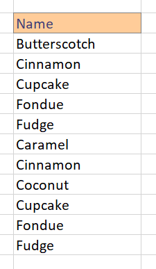
For example, take a look at my list of items below

.

It is easy with the Excel Unique Function to now return a list of Unique names from this list. The formula =UNIQUE(B3:B13) .  As illustrated below.

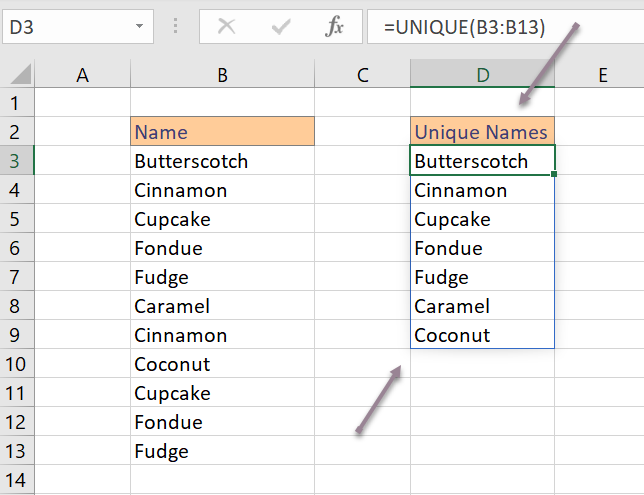
Excel will ‘spill’ the unique names and create a new array for you.

Extracting Unique Values From COLUMN Array.

Do note, however, that by not using the optional argument of By_Col, the argument has defaulted to FALSE which will return unique ROWS. If my array was in columns then I would simply adjust the formula to set the By_Col to TRUE. I have adjusted the array to COLUMNS. 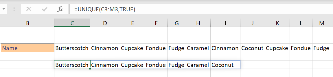So, as you can see it is really easy to extract our UNIQUE values. There is one other argument which is also optional which can give us another flavor of the Function. It is the Exactly_Once argument. What is that?. Well, this option will determine how the function deals with repeating values. By leaving the default to FALSE, Excel will extract unique values regardless of how many times they appear in the array or source of data. If we set this optional argument to FALSE then this now changes things a LOT. The UNIQUE function will extract ONLY VALUES THAT APPEAR ONCE.

Finally, let’s test this out with our data set.  Moving back to my example column of data.  If we want to return only those values that appear once then the formula is

=UNIQUE(B3:B13,FALSE,TRUE)

How easy is that?.   An Excel array function that is now available to most Excel users.  It is part of a new release of array functions.  

What Next? Want More Tips?

So, if you want more tips then sign up for my Monthly Newsletter where I share three Excel tips every month and receive my free Ebook, 50 Excel Tips.

Do You Need Help With An Excel Problem?.

Finally, I am pleased to announce I have teamed up with Excel Rescue, where you can get help FAST.  All you need to do is choose the Excel task that most closely describes what you need to be done.  Above all, there is a money-back guarantee and similarly Security and Non-Disclosure Agreements.  Try It!.  Need Help With An Excel VBA Macro?.  Of course, you don’t need to ask how to list all files in a directory as it is right here for free.  

Author: Oscar Cronquist Article last updated on January 26, 2023

The UNIQUE function is a very versatile Excel function, it lets you extract both unique and unique distinct values and also compare columns to columns or rows to rows.

The UNIQUE function is in the Lookup and reference category and is only available to Excel 365 subscribers.

1. UNIQUE Function Syntax

UNIQUE(array,[by_col],[exactly_once])

2. UNIQUE Function Arguments

Argument	Text
array	Required. Cell range or array.
[by_col]	Optional. Boolean value: True or False. True — Compares columns. False (default) — Compares rows.
[exactly_once]	Optional. Boolean value: True or False. True — Unique rows or columns False — Unique distinct rows or columns.

3. UNIQUE Function example

Formula in cell D3:

=UNIQUE(B3:B16)

4.0 Unique distinct values

Unique distinct values are all values except that duplicate values are merged into one distinct value.

Formula in cell D3:

=UNIQUE(B3:B5)

The UNIQUE function returns unique distinct values if you only use the first argument with a single-column cell range. The second and third arguments are optional.

Why does the UNIQUE function return a #NAME? error?

First, make sure you spelled the UNIQUE function correctly. If the UNIQUE function still returns a #NAME? error you probably own an earlier Excel version and can’t use it unless you upgrade to Excel 365.

There is a small formula you can use if you don’t have access to the UNIQUE function, check it out here: How to extract unique distinct values from a column [Formula]

Is the UNIQUE function available for Excel 2003, 2007, 2010, 2013, 2016, and 2019 users?

No, only Excel 365 subscribers have it. However, I made a small formula that works fine, check it out here: How to extract unique distinct values from a column [Formula]

Why does the UNIQUE function return a #SPILL! error?

The UNIQUE function returns an array of values and tries to automatically use the appropriate cell range needed to show all values. If one or more cells are occupied with other values the UNIQUE function returns #SPILL! error.

You have two options, delete or move the values that cause the error or deploy the UNIQUE function in another cell that has adjacent cells below empty.

Why does the UNIQUE function return a #CALC! error?

The UNIQUE function returns a #CALC! error if the output result has no values.

Can I use the UNIQUE function with an Excel Table and structured references?

Yes, you can. The UNIQUE function recalculates the output automatically if you add, edit or delete values in the Excel Table. It works fine with filtered Excel Tables as well.

Is the UNIQUE function case sensitive?

No, it is not case sensitive. Read theses articles if you need a case sensitive formula:

• Extract unique distinct values (case sensitive) [Formula]
• How to extract a case sensitive unique list from a column

Back to top

4.1 Extract unique distinct values sorted from A to Z

Formula in cell D3:

=UNIQUE(SORT(B3:B16))

Check out this article if you own an earlier Excel version and the SORT and UNIQUE functions are not available: Create a unique distinct alphabetically sorted list

Back to top

Explaining formula in cell D3

Step 1 — Sort values

The SORT function has the following arguments:
SORT(array,[sort_index],[sort_order],[by_col])

The first argument is required, the list is sorted from A to Z if the sort order is omitted.

SORT(B3:B16)

becomes

SORT({«Federer, Roger «; «Djokovic, Novak «; «Murray, Andy «; «Davydenko, Nikolay «; «Roddick, Andy «; «Del Potro, Juan Martin «; «Djokovic, Novak «; «Federer, Roger «; «Verdasco, Fernando «; «Murray, Andy «; «Del Potro, Juan Martin «; «Verdasco, Fernando «; «Djokovic, Novak «; «Roddick, Andy «})

and returns

{«Davydenko, Nikolay «;»Del Potro, Juan Martin «;»Del Potro, Juan Martin «;»Djokovic, Novak «;»Djokovic, Novak «;»Djokovic, Novak «;»Federer, Roger «;»Federer, Roger «;»Murray, Andy «;»Murray, Andy «;»Roddick, Andy «;»Roddick, Andy «;»Verdasco, Fernando «;»Verdasco, Fernando «}

Step 2 — Extract unique values

UNIQUE(SORT(B3:B16))

becomes

UNIQUE({«Davydenko, Nikolay «;»Del Potro, Juan Martin «;»Del Potro, Juan Martin «;»Djokovic, Novak «;»Djokovic, Novak «;»Djokovic, Novak «;»Federer, Roger «;»Federer, Roger «;»Murray, Andy «;»Murray, Andy «;»Roddick, Andy «;»Roddick, Andy «;»Verdasco, Fernando «;»Verdasco, Fernando «})

and returns

{«Davydenko, Nikolay «; «Del Potro, Juan Martin «; «Djokovic, Novak «; «Federer, Roger «; «Murray, Andy «; «Roddick, Andy «; «Verdasco, Fernando «}

The UNIQUE function may return an array if more than one value is returned. This will make the formula expand automatically to adjacent cells as far as needed.

Back to top

How do I return a unique distinct list sorted from Z to A?

Formula in cell D3:

=UNIQUE(SORT(B3:B16,,-1))

Back to top

4.2 Extract unique distinct values ignoring blanks

Formula in cell D3:

=UNIQUE(FILTER(B3:B16,B3:B16<>»»))

Check out this article if you own an earlier Excel version and the FILTER and UNIQUE functions are not available: Extract a unique distinct list and ignore blanks

Explaining formula in cell D3

Step 1 — Filter non-empty values

The FILTER function is available for Excel 365 subscribers, it has the following arguments:
FILTER(array,include,[if_empty])

The first argument is the cell range to be filtered, the second argument is the condition or criteria.

FILTER(B3:B16,B3:B16<>»»)

becomes

FILTER({«Federer, Roger «; «Djokovic, Novak «; «»; «Davydenko, Nikolay «; «Roddick, Andy «; «Del Potro, Juan Martin «; «Djokovic, Novak «; «Federer, Roger «; «»; «Murray, Andy «; «Del Potro, Juan Martin «; «Verdasco, Fernando «; «Djokovic, Novak «; «Roddick, Andy «},B3:B16<>»»)

becomes

FILTER({«Federer, Roger «; «Djokovic, Novak «; «»; «Davydenko, Nikolay «; «Roddick, Andy «; «Del Potro, Juan Martin «; «Djokovic, Novak «; «Federer, Roger «; «»; «Murray, Andy «; «Del Potro, Juan Martin «; «Verdasco, Fernando «; «Djokovic, Novak «; «Roddick, Andy «},{«Federer, Roger «; «Djokovic, Novak «; «»; «Davydenko, Nikolay «; «Roddick, Andy «; «Del Potro, Juan Martin «; «Djokovic, Novak «; «Federer, Roger «; «»; «Murray, Andy «; «Del Potro, Juan Martin «; «Verdasco, Fernando «; «Djokovic, Novak «; «Roddick, Andy «}<>»»)

becomes

FILTER{«Federer, Roger «; «Djokovic, Novak «; «»; «Davydenko, Nikolay «; «Roddick, Andy «; «Del Potro, Juan Martin «; «Djokovic, Novak «; «Federer, Roger «; «»; «Murray, Andy «; «Del Potro, Juan Martin «; «Verdasco, Fernando «; «Djokovic, Novak «; «Roddick, Andy «},{TRUE; TRUE; FALSE; TRUE; TRUE; TRUE; TRUE; TRUE; FALSE; TRUE; TRUE; TRUE; TRUE; TRUE})

and returns

{«Federer, Roger «;»Djokovic, Novak «;»Davydenko, Nikolay «;»Roddick, Andy «;»Del Potro, Juan Martin «;»Djokovic, Novak «;»Federer, Roger «;»Murray, Andy «;»Del Potro, Juan Martin «;»Verdasco, Fernando «;»Djokovic, Novak «;»Roddick, Andy «}

Step 2 — Extract unique distinct values

UNIQUE(FILTER(B3:B16,B3:B16<>»»))

becomes

UNIQUE({«Federer, Roger «;»Djokovic, Novak «;»Davydenko, Nikolay «;»Roddick, Andy «;»Del Potro, Juan Martin «;»Djokovic, Novak «;»Federer, Roger «;»Murray, Andy «;»Del Potro, Juan Martin «;»Verdasco, Fernando «;»Djokovic, Novak «;»Roddick, Andy «})

and returns

{«Federer, Roger «; «Djokovic, Novak «; «Davydenko, Nikolay «; «Roddick, Andy «; «Del Potro, Juan Martin «; «Murray, Andy «; «Verdasco, Fernando «}

Back to top

4.3 Extract unique distinct values sorted from A to Z ignoring blanks

Formula in cell D3:

=SORT(UNIQUE(FILTER(B3:B16,B3:B16<>»»)))

Check out this article if you own an earlier Excel version and the FILTER and UNIQUE functions are not available:
Create a unique distinct sorted list containing both numbers text removing blanks

Explaining formula in cell D3

Step 1 — Filter non-empty values

The FILTER function is available for Excel 365 subscribers, it has the following arguments:
FILTER(array,include,[if_empty])

The first argument is the cell range to be filtered, the second argument is the condition or criteria.

FILTER(B3:B16,B3:B16<>»»)

becomes

FILTER({«Federer, Roger «; «Djokovic, Novak «; «»; «Davydenko, Nikolay «; «Roddick, Andy «; «Del Potro, Juan Martin «; «Djokovic, Novak «; «Federer, Roger «; «»; «Murray, Andy «; «Del Potro, Juan Martin «; «Verdasco, Fernando «; «Djokovic, Novak «; «Roddick, Andy «},B3:B16<>»»)

becomes

FILTER({«Federer, Roger «; «Djokovic, Novak «; «»; «Davydenko, Nikolay «; «Roddick, Andy «; «Del Potro, Juan Martin «; «Djokovic, Novak «; «Federer, Roger «; «»; «Murray, Andy «; «Del Potro, Juan Martin «; «Verdasco, Fernando «; «Djokovic, Novak «; «Roddick, Andy «},{«Federer, Roger «; «Djokovic, Novak «; «»; «Davydenko, Nikolay «; «Roddick, Andy «; «Del Potro, Juan Martin «; «Djokovic, Novak «; «Federer, Roger «; «»; «Murray, Andy «; «Del Potro, Juan Martin «; «Verdasco, Fernando «; «Djokovic, Novak «; «Roddick, Andy «}<>»»)

becomes

FILTER{«Federer, Roger «; «Djokovic, Novak «; «»; «Davydenko, Nikolay «; «Roddick, Andy «; «Del Potro, Juan Martin «; «Djokovic, Novak «; «Federer, Roger «; «»; «Murray, Andy «; «Del Potro, Juan Martin «; «Verdasco, Fernando «; «Djokovic, Novak «; «Roddick, Andy «},{TRUE; TRUE; FALSE; TRUE; TRUE; TRUE; TRUE; TRUE; FALSE; TRUE; TRUE; TRUE; TRUE; TRUE})

and returns

{«Federer, Roger «;»Djokovic, Novak «;»Davydenko, Nikolay «;»Roddick, Andy «;»Del Potro, Juan Martin «;»Djokovic, Novak «;»Federer, Roger «;»Murray, Andy «;»Del Potro, Juan Martin «;»Verdasco, Fernando «;»Djokovic, Novak «;»Roddick, Andy «}

Step 2 — Extract unique distinct values

UNIQUE(FILTER(B3:B16,B3:B16<>»»))

becomes

UNIQUE({«Federer, Roger «;»Djokovic, Novak «;»Davydenko, Nikolay «;»Roddick, Andy «;»Del Potro, Juan Martin «;»Djokovic, Novak «;»Federer, Roger «;»Murray, Andy «;»Del Potro, Juan Martin «;»Verdasco, Fernando «;»Djokovic, Novak «;»Roddick, Andy «})

and returns

{«Federer, Roger «; «Djokovic, Novak «; «Davydenko, Nikolay «; «Roddick, Andy «; «Del Potro, Juan Martin «; «Murray, Andy «; «Verdasco, Fernando «}

Step 3 — Sort values

The SORT function has the following arguments: SORT(array,[sort_index],[sort_order],[by_col])

The first argument is required, the list is sorted from A to Z if the sort order is omitted.

SORT(UNIQUE(FILTER(B3:B16,B3:B16<>»»)))

becomes

SORT({«Federer, Roger «; «Djokovic, Novak «; «Davydenko, Nikolay «; «Roddick, Andy «; «Del Potro, Juan Martin «; «Murray, Andy «; «Verdasco, Fernando «})

and returns

{«Davydenko, Nikolay «; «Del Potro, Juan Martin «; «Djokovic, Novak «; «Federer, Roger «; «Murray, Andy «; «Roddick, Andy «; «Verdasco, Fernando «}

Back to top

4.4 Count unique distinct values

Formula in cell F3:

=ROWS(UNIQUE(B3:B16))

The formula above works fine if your cell range doesn’t contain any blank cells, the formula below takes care of blanks.

Formula in cell F3:

=ROWS(UNIQUE(FILTER(B3:B16,B3:B16<>»»)))

The ROWS function counts the number of rows that the UNIQUE function returns, that number is how many distinct values there are in cell range B3:B16.

This article explains a formula that works for earlier Excel versions: Count unique distinct values

Back to top

5.0 Unique values

Unique values are values that exist only once in a list. The image above shows a list in column B. Item «AA» has a duplicate and is not unique, however, item «BB» exists only once and is unique.

5.1 Extract unique values

Formula in cell D3:

=UNIQUE(B3:B15,,TRUE)

UNIQUE(array, [by_col], [exactly_once])

The third argument takes logical values True or False. True means unique value, in other words, values that only exist once in the list. False means extracting unique distinct values.

There are only two different values that exist once in cell range B3:B15. All other values have duplicates.

Check out this article if you own an earlier Excel version and the UNIQUE function is not available:
How to filter unique values from a list [Formula]

Back to top

5.2 Extract unique values sorted from A to Z

Formula in cell D3:

=SORT(UNIQUE(B3:B14,,TRUE))

Check out this article if you own an earlier Excel version and the UNIQUE function is not available: Filter unique values sorted from A to Z

Explaining formula in cell D3

Step 1 — Extract unique values

The UNIQUE function has the following arguments:
UNIQUE(array,[by_col],[exactly_once])

UNIQUE(B3:B14,,TRUE)

becomes

UNIQUE({«Federer, Roger «; «Djokovic, Novak «; «Murray, Andy «; «Davydenko, Nikolay «; «Roddick, Andy «; «Del Potro, Juan Martin «; «Djokovic, Novak «; «Verdasco, Fernando «; «Murray, Andy «; «Del Potro, Juan Martin «; «Djokovic, Novak «; «Roddick, Andy «},,TRUE)

and returns

{«Federer, Roger «;»Davydenko, Nikolay «;»Verdasco, Fernando «}

Step 2 — Sort values

The SORT function has the following arguments:
SORT(array,[sort_index],[sort_order],[by_col])

The first argument is required, the list is sorted from A to Z if the sort order is omitted.

SORT(UNIQUE(B3:B14,,TRUE))

becomes

SORT({«Federer, Roger «;»Davydenko, Nikolay «;»Verdasco, Fernando «})

and returns

{«Davydenko, Nikolay «; «Federer, Roger «; «Verdasco, Fernando «}

Back to top

5.3 Extract unique values ignoring blanks

The UNIQUE function returns 0 (zero) if there is exactly one blank in the list, however, it disappears if there are two or more blanks in the list.

To remove the blank use the following formula.

Formula in cell D3:

=UNIQUE(FILTER(B3:B16, B3:B16<>»»), , TRUE)

Check out this article if you own an earlier Excel version and the UNIQUE function is not available: How to filter unique values from a list [Formula] It works fine with blanks.

Explaining formula in cell D3

Step 1 — Filter non-empty values

The FILTER function is available for Excel 365 subscribers, it has the following arguments:
FILTER(array,include,[if_empty])

The first argument is the cell range to be filtered, the second argument is the condition or criteria.

FILTER(B3:B16,B3:B16<>»»)

becomes

FILTER({«Federer, Roger «; «Djokovic, Novak «; «Murray, Andy «; «Davydenko, Nikolay «; «Roddick, Andy «; «Del Potro, Juan Martin «; «Djokovic, Novak «; «»; «Verdasco, Fernando «; «Murray, Andy «; «Del Potro, Juan Martin «; «Verdasco, Fernando «; «Djokovic, Novak «; «Roddick, Andy «},{«Federer, Roger «; «Djokovic, Novak «; «Murray, Andy «; «Davydenko, Nikolay «; «Roddick, Andy «; «Del Potro, Juan Martin «; «Djokovic, Novak «; «»; «Verdasco, Fernando «; «Murray, Andy «; «Del Potro, Juan Martin «; «Verdasco, Fernando «; «Djokovic, Novak «; «Roddick, Andy «}<>»»)

becomes

FILTER({«Federer, Roger «; «Djokovic, Novak «; «Murray, Andy «; «Davydenko, Nikolay «; «Roddick, Andy «; «Del Potro, Juan Martin «; «Djokovic, Novak «; «»; «Verdasco, Fernando «; «Murray, Andy «; «Del Potro, Juan Martin «; «Verdasco, Fernando «; «Djokovic, Novak «; «Roddick, Andy «}, {«Federer, Roger «; «Djokovic, Novak «; «Murray, Andy «; «Davydenko, Nikolay «; «Roddick, Andy «; «Del Potro, Juan Martin «; «Djokovic, Novak «; «»; «Verdasco, Fernando «; «Murray, Andy «; «Del Potro, Juan Martin «; «Verdasco, Fernando «; «Djokovic, Novak «; «Roddick, Andy «}<>»»)

and returns

{«Federer, Roger «;»Djokovic, Novak «;»Murray, Andy «;»Davydenko, Nikolay «;»Roddick, Andy «;»Del Potro, Juan Martin «;»Djokovic, Novak «;»Verdasco, Fernando «;»Murray, Andy «;»Del Potro, Juan Martin «;»Verdasco, Fernando «;»Djokovic, Novak «;»Roddick, Andy «}

Step 2 — Extract unique values

The UNIQUE function has the following arguments:
UNIQUE(array,[by_col],[exactly_once])

UNIQUE(FILTER(B3:B16,B3:B16<>»»),,TRUE)

becomes

UNIQUE({«Federer, Roger «;»Djokovic, Novak «;»Murray, Andy «;»Davydenko, Nikolay «;»Roddick, Andy «;»Del Potro, Juan Martin «;»Djokovic, Novak «;»Verdasco, Fernando «;»Murray, Andy «;»Del Potro, Juan Martin «;»Verdasco, Fernando «;»Djokovic, Novak «;»Roddick, Andy «},,TRUE)

and returns

{«Federer, Roger «;»Davydenko, Nikolay «}

Back to top

5.4 Extract unique values sorted from A to Z ignoring blanks

Formula in cell D3:

=SORT(UNIQUE(FILTER(B3:B16,B3:B16<>»»),,TRUE))

Check out this article if you own an earlier Excel version and the UNIQUE function is not available: Filter unique values sorted from A to Z It seems to work fine with blanks.

Explaining formula in cell D3

Step 1 — Filter non-empty values

The FILTER function is available for Excel 365 subscribers, it has the following arguments:
FILTER(array,include,[if_empty])

The first argument is the cell range to be filtered, the second argument is the condition or critera.

FILTER(B3:B16,B3:B16<>»»)

becomes

FILTER({«Federer, Roger «; «Djokovic, Novak «; «Murray, Andy «; «Davydenko, Nikolay «; «Roddick, Andy «; «Del Potro, Juan Martin «; «Djokovic, Novak «; «»; «Verdasco, Fernando «; «Murray, Andy «; «Del Potro, Juan Martin «; «Verdasco, Fernando «; «Djokovic, Novak «; «Roddick, Andy «},{«Federer, Roger «; «Djokovic, Novak «; «Murray, Andy «; «Davydenko, Nikolay «; «Roddick, Andy «; «Del Potro, Juan Martin «; «Djokovic, Novak «; «»; «Verdasco, Fernando «; «Murray, Andy «; «Del Potro, Juan Martin «; «Verdasco, Fernando «; «Djokovic, Novak «; «Roddick, Andy «}<>»»)

becomes

FILTER({«Federer, Roger «; «Djokovic, Novak «; «Murray, Andy «; «Davydenko, Nikolay «; «Roddick, Andy «; «Del Potro, Juan Martin «; «Djokovic, Novak «; «»; «Verdasco, Fernando «; «Murray, Andy «; «Del Potro, Juan Martin «; «Verdasco, Fernando «; «Djokovic, Novak «; «Roddick, Andy «}, {«Federer, Roger «; «Djokovic, Novak «; «Murray, Andy «; «Davydenko, Nikolay «; «Roddick, Andy «; «Del Potro, Juan Martin «; «Djokovic, Novak «; «»; «Verdasco, Fernando «; «Murray, Andy «; «Del Potro, Juan Martin «; «Verdasco, Fernando «; «Djokovic, Novak «; «Roddick, Andy «}<>»»)

and returns

{«Federer, Roger «;»Djokovic, Novak «;»Murray, Andy «;»Davydenko, Nikolay «;»Roddick, Andy «;»Del Potro, Juan Martin «;»Djokovic, Novak «;»Verdasco, Fernando «;»Murray, Andy «;»Del Potro, Juan Martin «;»Verdasco, Fernando «;»Djokovic, Novak «;»Roddick, Andy «}

Step 2 — Extract unique values

The UNIQUE function has the following arguments: UNIQUE(array,[by_col],[exactly_once])

UNIQUE(FILTER(B3:B16,B3:B16<>»»),,TRUE)

becomes

UNIQUE({«Federer, Roger «;»Djokovic, Novak «;»Murray, Andy «;»Davydenko, Nikolay «;»Roddick, Andy «;»Del Potro, Juan Martin «;»Djokovic, Novak «;»Verdasco, Fernando «;»Murray, Andy «;»Del Potro, Juan Martin «;»Verdasco, Fernando «;»Djokovic, Novak «;»Roddick, Andy «},,TRUE)

and returns

{«Federer, Roger «;»Davydenko, Nikolay «}

Step 3 — Sort values

The SORT function has the following arguments:
SORT(array,[sort_index],[sort_order],[by_col])

The first argument is required, the list is sorted from A to Z if the sort order is omitted.

SORT(UNIQUE(FILTER(B3:B16,B3:B16<>»»),,TRUE))

becomes

SORT({«Federer, Roger «;»Davydenko, Nikolay «})

and returns

{«Davydenko, Nikolay»; Federer, Roger «}

Back to top

6.0 Unique distinct rows

Unique distinct rows are all rows except that duplicate rows are merged to one value.

Back to top

6.1 Extract unique distinct rows

Formula in cell E3:

=UNIQUE(B3:C6)

Check out this article if you own an earlier Excel version and the UNIQUE function returns a #NAME! error:
Filter unique distinct records

The UNIQUE function recognizes automatically a multicolumn cell range and returns unique distinct rows. The image above shows the UNIQUE function returning three rows, row 4 and 6 are merged into one row.

Back to top

6.2 Extract unique distinct rows ignoring blank rows

Formula in cell E3:

=UNIQUE(FILTER(B3:C6, (C3:C6<>»») * (B3:B6<>»»)))

Check out this article if you own an earlier Excel version and the UNIQUE function returns a #NAME! error:
Filter unique distinct row ignore blanks

Explaining formula in cell E3

Step 1 — Filter non-empty rows

The FILTER function is available for Excel 365 subscribers, it has the following arguments:
FILTER(array, include, [if_empty])

The first argument is the cell range to be filtered, the second argument is the condition or criteria.

FILTER(B3:C6, (C3:C16<>»») * (B3:B6<>»»)

becomes

FILTER({«AA», 1; «BB», 2; «AA», 2; «», «»; «BB», 2}, ({1; 2; 2; «»; 2}<>»»)*({«AA»; «BB»; «AA»; «»; «BB»}<>»»))

becomes

FILTER({«AA», 1; «BB», 2; «AA», 2; «», «»; «BB», 2}, {1;1;1;0;1})

and returns

{«AA», 1; «BB», 2; «AA», 2; «BB», 2}

Step 2 — Extract unique distinct rows

UNIQUE(FILTER(B3:C16,(C3:C16<>»»)*(B3:B16<>»»)))

becomes

UNIQUE({«AA», 1; «BB», 2; «AA», 2; «BB», 2})

and returns

{«AA», 1; «BB», 2; «AA», 2}

Back to top

6.3 Extract unique distinct rows sorted from A to Z ignoring blank rows

Formula in cell E3:

=LET(x, UNIQUE(FILTER(B3:C7, (C3:C7<>»»)*(B3:B7<>»»)), FALSE), SORTBY(x, INDEX(x, 0, 1), , INDEX(x, 0, 2), ))

This formula sorts the array based on the first column and then on the second column.

Explaining formula in cell E3

Step 1 — Filter non-empty rows

The FILTER function is available for Excel 365 subscribers, it has the following arguments: FILTER(array, include, [if_empty])

The first argument is the cell range to be filtered, the second argument is the condition or criteria.

FILTER(B3:C7, (C3:C7<>»»)*(B3:B7<>»»))

becomes

FILTER({«AA», 1; «BB», 2; «AA», 2; «», «»; «BB», 2}, ({1; 2; 2; «»; 2}<>»»)*({«AA»; «BB»; «AA»; «»; «BB»}<>»»))

becomes

FILTER({«AA», 1; «BB», 2; «AA», 2; «», «»; «BB», 2}, {1;1;1;0;1})

and returns

{«AA», 1; «BB», 2; «AA», 2; «BB», 2}

Step 2 — Extract unique distinct rows

UNIQUE(FILTER(B3:C7, (C3:C7<>»»)*(B3:B7<>»»)))

becomes

UNIQUE({«AA», 1; «BB», 2; «AA», 2; «BB», 2})

and returns

{«AA», 1; «AA», 2; «BB», 2}

Step 3 — Sort array

The SORTBY function lets you sort a multicolumn cell range based on the order of columns you define.

SORTBY(UNIQUE(FILTER(B3:C7, (C3:C7<>»»)*(B3:B7<>»»)), INDEX(UNIQUE(FILTER(B3:C7, (C3:C7<>»»)*(B3:B7<>»»)), 0, 1), , INDEX(UNIQUE(FILTER(B3:C7, (C3:C7<>»»)*(B3:B7<>»»)), 0, 2), )

becomes

SORTBY({«AA», 1; «BB», 2; «AA», 2}, INDEX({«AA», 1; «BB», 2; «AA», 2}, 0, 1), , INDEX({«AA», 1; «BB», 2; «AA», 2}, 0, 2), )

becomes

SORTBY({«AA», 1; «BB», 2; «AA», 2}, {«AA»;»BB»;»AA»}, , {1;2;2}, )

and returns

{«AA»,1;»AA»,2;»BB»,2}

Step 4 — Shorten formula

The LET function lets you name an expression that is repeated often in the formula, this allows you to shorten the formula considerably.

SORTBY(UNIQUE(FILTER(B3:C7, (C3:C7<>»»)*(B3:B7<>»»)), INDEX(UNIQUE(FILTER(B3:C7, (C3:C7<>»»)*(B3:B7<>»»)), 0, 1), , INDEX(UNIQUE(FILTER(B3:C7, (C3:C7<>»»)*(B3:B7<>»»)), 0, 2), )

x — UNIQUE(FILTER(B3:C7, (C3:C7<>»»)*(B3:B7<>»»)), FALSE)

LET(x, UNIQUE(FILTER(B3:C7, (C3:C7<>»»)*(B3:B7<>»»)), FALSE), SORTBY(x, INDEX(x, 0, 1), , INDEX(x, 0, 2), ))

Back to top

7.0 Unique rows

Unique rows are rows that exist only once in a cell range. The image above shows that B4:C4 and B6:D6 are duplicates and are not in the result in cell range E3:F4.

Back to top

7.1 Extract unique rows

Formula in cell E3:

=UNIQUE(B3:C6,,TRUE)

The third argument in the UNIQUE function determines if rows that exist exactly once should be extracted.
UNIQUE(array,[by_col],[exactly_once]) Default is False. The formula above is entered as a regular formula.

The following array formula works for older Excel versions than Excel 365.

Array formula in cell E3:

=INDEX($B$3:$C$6, SMALL(IF(COUNTIFS($B$3:$B$6, $B$3:$B$6, $C$3:$C$6, $C$3:$C$6)=1, MATCH(ROW($B$3:$B$6), ROW($B$3:$B$6)), «»), ROWS($A$1:A1)), COLUMNS($A$1:A1))

How to enter an array formula

These steps are for earlier Excel versions.

1. Copy the above array formula.
2. Double-press with left mouse button on cell E3.
3. Paste array formula.
4. Press and hold CTRL + SHIFT simultaneously.
5. Press Enter.
6. Release all keys.

Back to top

7.2 Extract unique rows ignoring blank rows

Formula in cell E3:

=UNIQUE(FILTER(B3:C8, (C3:C8<>»»)*(B3:B8<>»»)), FALSE, TRUE)

The formula above is entered as a regular formula.

The following array formula works for older Excel versions than Excel 365.

Array formula in cell E3:

=INDEX($B$3:$C$6, SMALL(IF(COUNTIFS($B$3:$B$6, $B$3:$B$6, $C$3:$C$6, $C$3:$C$6)=1, MATCH(ROW($B$3:$B$6), ROW($B$3:$B$6)), «»), ROWS($A$1:A1)), COLUMNS($A$1:A1))

How to enter an array formula

1. Copy the above array formula.
2. Double-press with left mouse button on cell E3.
3. PAste array formula.
4. Press and hold CTRL + SHIFT simultaneously.
5. Press Enter.
6. Release all keys.

Explaining Excel 365 formula in cell E3

Step 1 — Filter non-empty values

The FILTER function is available for Excel 365 subscribers, it has the following arguments:
FILTER(array, include, [if_empty])

The first argument is the cell range to be filtered, the second argument is the condition or criteria.

FILTER(B3:C8,(C3:C8<>»»)*(B3:B8<>»»))

becomes

FILTER({«AA», 1; «BB», 2; «», «»; «AA», 2; «BB», 2; «», «»},({1; 2; «»; 2; 2; «»}<>»»)*({«AA»; «BB»; «»; «AA»; «BB»; «»}<>»»))

becomes

FILTER({«AA», 1; «BB», 2; «», «»; «AA», 2; «BB», 2; «», «»}, {1;1;0;1;1;0})

and returns

{«AA», 1; «BB», 2; «AA», 2; «BB», 2}

Step 2 — Extract unique rows

The third argument in the UNIQUE function determines if rows that exist exactly once should be extracted.
UNIQUE(array,[by_col],[exactly_once]) Default is False meaning distinct values (not unique).

UNIQUE(FILTER(B3:C8, (C3:C8<>»»)*(B3:B8<>»»)), FALSE, TRUE)

becomes

UNIQUE({«AA», 1; «BB», 2; «AA», 2; «BB», 2}, FALSE, TRUE)

and returns

{«AA», 1; «AA», 2}

Back to top

7.3 Extract unique rows sorted from A to Z ignoring blank rows

This formula sorts the data set based on the first column (B) and the on the second column (C).

Formula in cell E3:

=LET(x, UNIQUE(FILTER(B3:C8, (C3:C8<>»»)*(B3:B8<>»»)), , TRUE), SORTBY(x, INDEX(x, 0, 1), , INDEX(x, 0, 2), ))

The formula above is entered as a regular formula.

Explaining formula in cell E3

Step 1 — Filter non-empty values

The FILTER function is available for Excel 365 subscribers, it has the following arguments:
FILTER(array, include, [if_empty])

The first argument is the cell range to be filtered, the second argument is the condition or criteria.

FILTER(B3:C8, (C3:C8<>»»)*(B3:B8<>»»))

becomes

FILTER({«AA», 2; «BB», 2; 0, 0; «AA», 1; «BB», 2; 0, 0}, ({2;2;0;1;2;0}<>»»)*({«AA»;»BB»;0;»AA»;»BB»;0}<>»»))

becomes

FILTER({«AA», 2; «BB», 2; 0, 0; «AA», 1; «BB», 2; 0, 0},{1;1;0;1;1;0})

and returns

{«AA», 2; «BB», 2; «AA», 1; «BB», 2}

Step 2 — Extract unique rows

The third argument in the UNIQUE function determines if rows that exist exactly once should be extracted.
UNIQUE(array,[by_col],[exactly_once]) Default is False meaning distinct values (not unique).

UNIQUE(FILTER(B3:C8, (C3:C8<>»»)*(B3:B8<>»»)), , TRUE)

becomes

UNIQUE({«AA», 2; «BB», 2; «AA», 1; «BB», 2}, , TRUE)

and returns

{«AA», 2; «AA», 1}

Step 3 — Sort array

The SORTBY function lets you sort a multicolumn cell range based on the order of columns you define.
SORTBY(array, by_array1, [sort_order1], [by_array2, sort_order2],…)

SORTBY(UNIQUE(FILTER(B3:C8, (C3:C8<>»»)*(B3:B8<>»»)), , TRUE), INDEX(UNIQUE(FILTER(B3:C8, (C3:C8<>»»)*(B3:B8<>»»)), , TRUE), 0, 1), , INDEX(UNIQUE(FILTER(B3:C8, (C3:C8<>»»)*(B3:B8<>»»)), , TRUE), 0, 2), )

becomes

SORTBY({«AA», 2; «AA», 1}, INDEX({«AA», 2; «AA», 1}, 0, 1), , INDEX({«AA», 2; «AA», 1}, 0, 2), )

becomes

SORTBY({«AA», 2; «AA», 1}, {«AA»; «AA»}, , {2; 1}, )

and returns

{«AA», 1; «AA», 2}

Step 4 — Shrink formula

The LET function lets you name an expression that is repeated often in the formula, this allows you to shorten the formula considerably.

SORTBY(UNIQUE(FILTER(B3:C8, (C3:C8<>»»)*(B3:B8<>»»)), , TRUE), INDEX(UNIQUE(FILTER(B3:C8, (C3:C8<>»»)*(B3:B8<>»»)), , TRUE), 0, 1), , INDEX(UNIQUE(FILTER(B3:C8, (C3:C8<>»»)*(B3:B8<>»»)), , TRUE), 0, 2), )

This part: UNIQUE(FILTER(B3:C8, (C3:C8<>»»)*(B3:B8<>»»)), , TRUE) is repeated three times in the formula.

x — UNIQUE(FILTER(B3:C8, (C3:C8<>»»)*(B3:B8<>»»)), , TRUE)

LET(x, UNIQUE(FILTER(B3:C8, (C3:C8<>»»)*(B3:B8<>»»)), , TRUE), SORTBY(x, INDEX(x, 0, 1), , INDEX(x, 0, 2), ))

Back to top

8.0 Unique and unique distinct columns

Back to top

8.1 Extract unique distinct columns

Formula in cell E3:

=UNIQUE(C2:F3,TRUE)

The formula above is entered as a regular formula.

Back to top

8.2 Extract unique columns

Formula in cell E3:

=UNIQUE(C2:F3,TRUE,TRUE)

The formula above is entered as a regular formula.

Back to top

9.0 Get Excel file

Back to top