
Return value
A logical value (TRUE or FALSE)
Usage notes
The ISNUMBER function returns TRUE when a cell contains a number, and FALSE if not. You can use ISNUMBER to check that a cell contains a numeric value, or that the result of another function is a number.
The ISNUMBER function takes one argument, value, which can be a cell reference, a formula, or a hardcoded value. Typically, value is entered as a cell reference like A1. When value is a number, the ISNUMBER function will return TRUE. Otherwise, ISNUMBER will return FALSE.
Examples
The ISNUMBER function returns TRUE if value is numeric:
=ISNUMBER("apple") // returns FALSE
=ISNUMBER(100) // returns TRUE
If cell A1 contains the number 100, ISNUMBER returns TRUE:
=ISNUMBER(A1) // returns TRUE
If a cell contains a formula, ISNUMBER checks the result of the formula:
=ISNUMBER(2+2) // returns TRUE
=ISNUMBER(2^3) // returns TRUE
=ISNUMBER(10 &" apples") // returns FALSE
Note: the ampersand (&) is the concatenation operator in Excel. When values are concatenated, the result is text.
Count numeric values
To count cells in a range that contain numbers, you can use the SUMPRODUCT function like this:
=SUMPRODUCT(--ISNUMBER(range))
The double negative coerces the TRUE and FALSE results from ISNUMBER into 1s and 0s and SUMPRODUCT sums the result.
Notes
- ISNUMBER will return TRUE for Excel dates and times since they are numeric.
- ISNUMBER will return FALSE for empty cells and errors.
Checks if a cell contains a number or not
What is the Excel ISNUMBER Function?
The Excel ISNUMBER Function[1] is categorized under Information functions. The function checks if a cell in Excel contains a number or not. It will return TRUE if the value is a number and if not, a FALSE value. For example, if the given value is a text, date, or time, it will return FALSE.
As a financial analyst, when dealing with large amounts of data, ISNUMBER Excel function helps in testing if a given result of a formula is a number or not.
Formula
=ISNUMBER(value)
The Excel ISNUMBER function uses the following arguments:
- Value (required argument) – This is the expression or value that needs to be tested. It is generally provided as a cell address.
The ISNUMBER Excel function will return a logical value, which is TRUE or FALSE.
How to use the ISNUMBER Excel Function?
To understand the uses of the ISNUMBER Excel function, let’s consider a few examples:
Example 1
Let’s first understand how the function behaves using the following set of data:
| Data | Formula | Result | Remark |
|---|---|---|---|
| 1 | =ISNUMBER(1) | TRUE | The value provided is a number, so the function returned TRUE. |
| TEXT | =ISNUMBER(TEXT) | FALSE | The function returns FALSE for text values. |
| 10/20 | =ISNUMBER(10/20) | TRUE | The formula will return a number, so the function returned TRUE. |
| #NAME? | =ISNUMBER(#NAME?) | FALSE | The function returned FALSE for formula errors. |
| =ISNUMBER( ) | FALSE | The result is FALSE, as it is not a number. |
Example 2 – Check if Excel contains a number in a cell
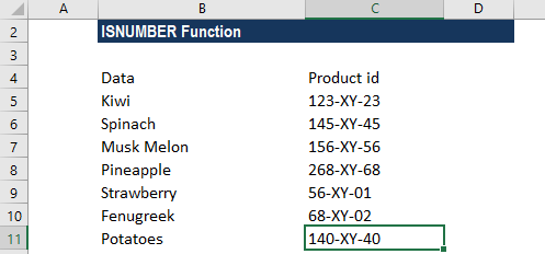
Suppose we wish to allow values that contain the text string XY. Using ISNUMBER along with data validation, we can check if Excel contains “XY” in the cell. Suppose we are given the following data:
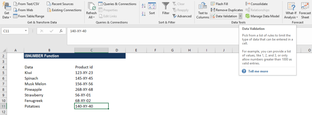
To allow only values that contain a specific text string, we can use data validation with a customized formula based on the FIND and ISNUMBER Excel functions. Essentially, it checks if Excel contains a number in the cell or not. To do this, we will apply data validation to C4:C11 cells. To apply the data validation, click on the Data tab, go to Data Tools, and click on Data Validation, as shown below:
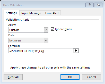
Now, select Data validation and click on Settings. As shown below, enter the formula =ISNUMBER(FIND(“XY”,C4)). To activate the formula cell, you need to choose Validation criteria – Allow – Custom.
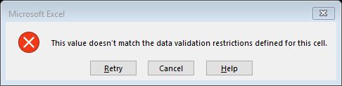
When someone tries to change XY into something else, data validation rules are triggered, particularly when a user adds or changes a cell value.
The FIND function is shaped to search for the text “XY” in cell C4. If found, FIND will return a numeric position (e.g., 2, 4, 5, etc.) for the starting point of the text in the cell. If the text is not found, FIND will return an error. For C4, FIND will return 5, since “XY” starts at character 5.
The result from using the FIND function above is then evaluated by the ISNUMBER Excel function. For any numeric result returned by FIND, ISNUMBER will return TRUE and validation will succeed. When text is not found, FIND will return an error, ISNUMBER will return FALSE, and the input will fail validation.
A few notes about the ISNUMBER Function
- The function is part of the IS functions that return the logical values TRUE or FALSE.
- The function doesn’t return any error such as #NAME!, #N/A!, etc., as it just evaluates data.
- The function was introduced in MS Excel 2000.
Click here to download the sample Excel file
Additional Resources
Thanks for reading CFI’s guide to important Excel functions! By taking the time to learn and master these functions, you’ll significantly speed up your financial analysis. To learn more, check out these additional CFI resources:
- Excel Functions for Finance
- Advanced Excel Formulas Course
- Advanced Excel Formulas You Must Know
- Excel Shortcuts for PC and Mac
- See all Excel resources
ISNUMBER Function in Excel
ISNUMBER function in excel is an information function that checks if the referred cell value is numeric or non-numeric. Its output is a boolean value (“True,” if the “value” parameter is numeric or “False” if the “value” parameter is non-numeric)
Syntax
The ISNUMBER formula is stated as follows:
You are free to use this image on your website, templates, etc, Please provide us with an attribution linkArticle Link to be Hyperlinked
For eg:
Source: ISNUMBER in Excel (wallstreetmojo.com)
The ISNUMBER formula has only one parameter, the “value.”
- Value: It is a flexible parameter. It can be another function or formula, a cell, or value that needs testing if it is numeric or not.
The ISNUMBER formula returns the following logical values:
- “True,” if the “value” parameter is numeric.
- “False,” if the “value” parameter is non-numeric.
The formula is represented in the following format.
“=ISNUMBER(Reference Cell)”
The argument “reference cell” refers to the cell which we want to check or identify.
Let us consider the following ISNUMBER formula.
“=ISNUMBER(T1XT)”
The output is “false,” as the argument T1XT does not have numbers in it.
Table of contents
- ISNUMBER Function in Excel
- Syntax
- Characteristics of ISNUMBER Function
- How to Use the ISNUMBER Function in Excel?
- How to use Excel ISNUMBER Function and the SEARCH Function?
- Frequently Asked Questions (FAQs)
- ISNUMBER in Excel Video
- Recommended Articles
Characteristics of ISNUMBER Function
- It returns a Boolean value (“true” or “false”).
- It finds its usage as a worksheet (WS) function.
- It is a part of IS functions group of Excel.
How to Use the ISNUMBER Function in Excel?
Let us understand the uses of this function with few examples of actual data.
You can download this ISNUMBER Function Excel Template here – ISNUMBER Function Excel Template
Let us enter a few values given in the table below and test the behavior of the ISNUMBER function.

How to use Excel ISNUMBER Function and the SEARCH Function?
The ISNUMBER function, together with the SEARCH function, checks if a cell contains a specific sub-string among the text string.
SEARCH function in ExcelSearch function gives the position of a substring in a given string when we give a parameter of the position to search from. As a result, this formula requires three arguments. The first is the substring, the second is the string itself, and the last is the position to start the search.read more will return the position (or index) of a specified substring within a text string. It belongs to the Excel TEXT functions category. It allows running a case-insensitive search on text and supports the usage of wild cards.
We will understand how the ISNUMBER function works together with the SEARCH function in the following example.
Let us use other functions (e.g., SEARCH function) as parameters for the ISNUMBER function and test its behavior (as shown in the table below).
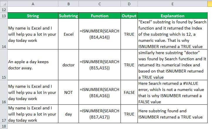
Consider the ISNUMBER formula mentioned in the table,
“=ISNUMBER(SEARCH(B14,A14))”
Now, we will observe how this formula works,
- At first, the SEARCH function looks for the substring “Excel” (B14) in the specified cell (A14). It returns the position of the substring as 12. If the substring is not found, it returns an error value (#VALUE).
- Then, the ISNUMBER function checks whether the SEARCH function returns a numeric value; if yes, the output is “true.” If the SEARCH shows an error value (non-numeric), then ISNUMBER returns “false.”
Frequently Asked Questions (FAQs)
What is the Excel ISNUMBER function?
The ISNUMBER function checks if a cell contains a number or not. It returns “true” if the value is numeric, and if not, it returns a “false.”
How to use ISNUMBER in Excel?
We use the ISNUMBER function to test if a value is a number. It will return “true” when the value is numeric and “false” when non-numeric.
Let us consider the syntax “=ISNUMBER(G1).” It returns “true” if the argument “G1” contains a number or a formula that returns a numeric value. It returns “false” if the argument “G1” contains the text.
How do ISNUMBER and ISTEXT functions differ?
The ISNUMBER function helps to check whether a value in a cell or a value resulting from another formula is a number. The output of ISNUMBER is either “true” or “false.”
The ISTEXT function checks whether a value is a text or not. The result of this function is also either “true” or “false.” Moreover, using this function, you can find if a value in a cell is a numeric value entered as text.
• The ISNUMBER function is an information function used to find if the cell value in reference is a numerical value or not. It returns values as “true” or “false.”
• The formula for the ISNUMBER function is “=ISNUMBER (value).”
• It is a worksheet (WS) function in Excel.
• It is a Boolean function of Excel which gives the output as “true” or “false.”
• The ISNUMBER function along with the Excel SEARCH function, checks if a cell contains a specific text among the content of the cell.
ISNUMBER in Excel Video
Recommended Articles
This is a guide to the ISNUMBER function in Excel. In this article, we have discussed how to use this function along with step-by-step examples and a downloadable template. You may also look at the below useful functions in Excel –
- Excel Auto NumberThere are two approaches for auto numbering. To begin, fill the first two cells with the series you wish to insert and drag it to the table’s end. Second, use the =ROW() formula to get the number, and then drag it to the table’s end.read more
- Numbering in ExcelNumbering in excel means providing a cell with numbers which are like serial numbers to some table, obviously it can also be done manually by filling first two cells with numbers and drag down to the end to table which excels will automatically fill the series.read more
- MAX in ExcelThe MAX Formula in Excel is used to calculate the maximum value from a set of data/array. It counts numbers but ignores empty cells, text, the logical values TRUE and FALSE, and text values.read more
- SUMPRODUCT Function in ExcelThe SUMPRODUCT excel function multiplies the numbers of two or more arrays and sums up the resulting products.read more
- Excel Shortcut Paste ValuesPasting values is a common procedure that allows us to eliminate any formatting and formulas from the copied cell and paste them into the pasted cell. «Alt + E + S + V» is the shortcut key for pasting values.read more
В учебнике объясняется, что такое ISNUMBER в Excel, и приводятся примеры базового и расширенного использования.
Концепция функции ЕЧИСЛО в Excel очень проста — она просто проверяет, является ли заданное значение числом или нет. Важным моментом здесь является то, что практическое использование функции выходит далеко за рамки ее основной концепции, особенно в сочетании с другими функциями в более крупных формулах.
Функция ЕЧИСЛО в Excel проверяет, содержит ли ячейка числовое значение или нет. Он относится к группе функций ИС.
Функция доступна во всех версиях Excel для Office 365, Excel 2019, Excel 2016, Excel 2013, Excel 2010, Excel 2007 и более ранних версиях.
Синтаксис ISNUMBER требует только одного аргумента:
=ЧИСЛО(значение)
Где ценность это значение, которое вы хотите проверить. Обычно он представлен ссылкой на ячейку, но вы также можете указать реальное значение или вложить другую функцию в ISNUMBER для проверки результата.
Если ценность является числовым, функция возвращает ИСТИНА. Для всего остального (текстовые значения, ошибки, пробелы) ISNUMBER возвращает FALSE.
В качестве примера, давайте проверим значения в ячейках с A2 по A6, и мы обнаружим, что первые 3 значения являются числами, а последние два — текстом:
2 вещи, которые вы должны знать о функции ISNUMBER в Excel
Здесь следует отметить несколько интересных моментов:
- Во внутреннем представлении Excel даты и время являются числовыми значениями, поэтому формула ЕЧИСЛО возвращает для них ИСТИНА (см. B3 и B4 на снимке экрана выше).
- Для чисел, сохраненных в виде текста, функция ЕЧИСЛО возвращает ЛОЖЬ (см. этот пример).
Примеры формулы ЕЧИСЛО в Excel
В приведенных ниже примерах показано несколько распространенных и несколько нетривиальных способов использования ISNUMBER в Excel.
Проверить, является ли значение числом
Если у вас есть множество значений на листе и вы хотите знать, какие из них являются числами, ISNUMBER — это правильная функция для использования.
В этом примере первое значение находится в A2, поэтому мы используем приведенную ниже формулу, чтобы проверить его, а затем перетащите формулу вниз на столько ячеек, сколько необходимо:
=ЧИСЛО(A2)
Обратите внимание, хотя все значения выглядят как числа, формула ЕЧИСЛО вернула ЛОЖЬ для ячеек A4 и A5, что означает, что эти значения являются числовыми строками, т. е. числами, отформатированными как текст. Для этого могут быть разные причины, например ведущие нули, предшествующий апостроф и т. д. Какой бы ни была причина, Excel не распознает такие значения как числа. Итак, если ваши значения не вычисляются правильно, первое, что вам нужно проверить, это действительно ли они являются числами с точки зрения Excel, а затем преобразовать текст в число, если это необходимо.
формула ПОИСК ISNUMBER в Excel
Помимо определения чисел функция ЕЧИСЛО Excel также может проверять, содержит ли ячейка определенный текст как часть содержимого. Для этого используйте ISNUMBER вместе с функцией SEARCH.
В общем виде формула выглядит следующим образом:
IНОМЕР(ПОИСК(подстрока, клетка))
Где подстрока это текст, который вы хотите найти.
В качестве примера давайте проверим, содержит ли строка в A3 определенный цвет, скажем, красный:
=ISNUMBER(ПОИСК(«красный», A3))
Эта формула хорошо работает для одной ячейки. Но поскольку наша примерная таблица (см. ниже) содержит три разных цвета, написание отдельной формулы для каждого из них было бы пустой тратой времени. Вместо этого мы будем ссылаться на ячейку, содержащую интересующий цвет (B2).
=ISNUMBER(ПОИСК(B$2, $A3))
Чтобы формула корректно копировалась вниз и вправо, обязательно зафиксируйте следующие координаты знаком $:
- В подстрока ссылку, заблокируйте строку (B$2), чтобы скопированные формулы всегда выбирали подстроки в строке 2. Ссылка на столбец является относительной, поскольку мы хотим, чтобы она корректировалась для каждого столбца, т. е. когда формула копируется в C3, ссылка на подстроку будет изменить на 2 канадских доллара.
- в исходная ячейка ссылку, заблокируйте столбец ($A3), чтобы все формулы проверяли значения в столбце A.
На скриншоте ниже показан результат:
ISNUMBER FIND — формула с учетом регистра
Так как функция ПОИСК без учета регистра, приведенная выше формула не различает прописные и строчные символы. Если вы ищете формулу с учетом регистра, используйте функцию НАЙТИ, а не ПОИСК.
IЧИСЛО(НАЙТИ(подстрока, клетка))
Для нашего примера набора данных формула будет иметь следующий вид:
=ЧИСЛО(НАЙТИ(B$2, $A3))
Как работает эта формула
Логика формулы вполне очевидна и проста для понимания:
- Функция ПОИСК/НАЙТИ ищет подстроку в указанной ячейке. Если подстрока найдена, возвращается позиция первого символа. Если подстрока не найдена, функция выдает ошибку #ЗНАЧ! ошибка.
- Функция ISNUMBER берет его оттуда и обрабатывает числовые позиции. Таким образом, если подстрока найдена и ее позиция возвращается в виде числа, ISNUMBER выводит TRUE. Если подстрока не найдена и #VALUE! возникает ошибка, ISNUMBER выводит FALSE.
ЕСЛИ ЕСЛИ ЕСЛИ ЧИСЛО формула
Если вы хотите получить формулу, которая выводит что-то отличное от ИСТИНА или ЛОЖЬ, используйте ЕСЛИЧИСЛО вместе с функцией ЕСЛИ.
Пример 1. Ячейка содержит какой текст
Продолжая предыдущий пример, предположим, что вы хотите пометить цвет каждого элемента знаком «x», как показано в таблице ниже.
Для этого просто оберните Формула ПОИСКА НОМЕРА в оператор ЕСЛИ:
=ЕСЛИ(ЧИСЛО(ПОИСК(B$2, $A3)), «x», «»)
Если ISNUMBER возвращает TRUE, функция ЕСЛИ выводит «x» (или любое другое значение, которое вы указываете для значение_если_истина аргумент). Если ISNUMBER возвращает FALSE, функция ЕСЛИ выводит пустую строку («»).
Пример 2. Первый символ в ячейке — число или текст
Представьте, что вы работаете со списком буквенно-цифровых строк и хотите знать, является ли первый символ строки цифрой или буквой.
Чтобы построить такую формулу, нам понадобятся 4 разные функции:
- Функция LEFT извлекает первый символ из начала строки, скажем, в ячейке A2:
ВЛЕВО(A2, 1)
- Поскольку LEFT относится к категории текстовых функций, ее результатом всегда является текстовая строка, даже если она содержит только числа. Поэтому перед проверкой извлеченного символа нам нужно попробовать преобразовать его в число. Для этого используйте либо функцию ЗНАЧ, либо двойной унарный оператор:
ЗНАЧЕНИЕ(ЛЕВО(A2, 1)) или (—ЛЕВО(A2, 1))
- Функция ISNUMBER определяет, является ли извлеченный символ числовым или нет:
IЧИСЛО(ЗНАЧЕНИЕ(ЛЕВО(A2, 1)))
- В зависимости от результата ISNUMBER (ИСТИНА или ЛОЖЬ) функция ЕСЛИ возвращает «Число» или «Букву» соответственно.
Предполагая, что мы тестируем строку в A2, полная формула принимает следующий вид:
=ЕСЛИ(ЧИСЛО(ЗНАЧЕНИЕ(ЛЕВО(A2, 1))), «Число», «Буква»)
или же
=ЕСЛИ(ЧИСЛО(—ЛЕВО(A2, 1)), «Число», «Буква»)
Функция ISNUMBER также удобна для извлечения чисел из строки. Вот пример: Получить число из любой позиции в строке.
Проверить, не является ли значение числом
Хотя в Microsoft Excel есть специальная функция ISNONTEXT, позволяющая определить, не является ли значение ячейки текстом, аналогичная функция для чисел отсутствует.
Простое решение — использовать ISNUMBER в сочетании с NOT, которое возвращает противоположное логическому значению. Другими словами, когда ISNUMBER возвращает TRUE, NOT преобразует его в FALSE, и наоборот.
Чтобы увидеть его в действии, обратите внимание на результаты следующей формулы:
=НЕ(ЧИСЛО(A2))
Другой подход заключается в совместном использовании функций ЕСЛИ и ЕСЛИЧИСЛО:
=ЕСЛИ(ЧИСЛО(A2), «», «Не число»)
Если A2 является числовым, формула ничего не возвращает (пустая строка). Если A2 не является числом, формула говорит об этом заранее: «Не число».
Если вы хотите выполнить некоторые вычисления с числами, поместите уравнение или другую формулу в поле значение_если_истина аргумент вместо пустой строки. Например, приведенная ниже формула будет умножать числа на 10 и давать «Не число» для нечисловых значений:
=ЕСЛИ(ЧИСЛО(A2), A2*10, «Не число»)
Проверьте, содержит ли диапазон какое-либо число
В ситуации, когда вы хотите проверить весь диапазон чисел, используйте функцию ЕСЧИСЛО в сочетании с СУММПРОИЗВ следующим образом:
СУММПРОИЗВ(—ЧИСЛО(диапазон))>0
СУММПРОИЗВ(ЧИСЛО(диапазон)*1)>0
Например, чтобы узнать, содержит ли диапазон A2:A5 какое-либо числовое значение, формулы будут выглядеть следующим образом:
=СУММПРОИЗВ(—ЧИСЛО(A2:A5))>0
=СУММПРОИЗВ(ЧИСЛО(A2:A5)*1)>0
Если вы хотите вывести «Да» и «Нет» вместо ИСТИНА и ЛОЖЬ, используйте оператор IF в качестве «оболочки» для приведенных выше формул. Например:
=ЕСЛИ(СУММПРОИЗВ(—ЧИСЛО(A2:A5))>0, «Да», «Нет»)
Как работает эта формула
В основе формулы функция ЕЧИСЛО оценивает каждую ячейку указанного диапазона, скажем, B2:B5, и возвращает ИСТИНА для чисел и ЛОЖЬ для всего остального. Поскольку диапазон содержит 4 ячейки, массив имеет 4 элемента:
{ИСТИНА; ЛОЖЬ; ЛОЖЬ; ЛОЖЬ}
Операция умножения или двойной унарный (—) преобразует ИСТИНА и ЛОЖЬ в 1 и 0 соответственно:
{1;0;0;0}
Функция СУММПРОИЗВ складывает элементы массива. Если результат больше нуля, это означает, что в диапазоне есть хотя бы одно число. Итак, вы используете «> 0», чтобы получить окончательный результат ИСТИНА или ЛОЖЬ.
ISNUMBER в условном форматировании для выделения ячеек, содержащих определенный текст
Если вы хотите выделить ячейки или целые строки, содержащие определенный текст, создайте правило условного форматирования на основе ПОИСК ПО НОМЕРУ (без учета регистра) или НАЙТИ НОМЕР (с учетом регистра) формула.
В этом примере мы собираемся выделить строки на основе значения в столбце A. Точнее, мы выделим элементы, содержащие слово «красный». Вот как:
- Выберите все строки данных (в этом примере A2: C6) или только столбец, в котором вы хотите выделить ячейки.
- На Дом вкладка, в Стили группа, нажмите Новое правило > Используйте формулу, чтобы определить, какие ячейки нужно отформатировать.
- в Форматировать значения, где эта формула верна введите приведенную ниже формулу (обратите внимание, что координата столбца заблокирована знаком $):
=ISNUMBER(ПОИСК(«красный», $A2))
- Нажмите на Формат кнопку и выберите нужный формат.
- Нажмите ОК дважды.
Если у вас мало опыта работы с условным форматированием Excel, вы можете найти подробные шаги со снимками экрана в этом руководстве: Как создать правило условного форматирования на основе формулы.
В результате подсвечиваются все элементы красного цвета:
Вместо «жесткого кодирования» цвета в правиле условного форматирования вы можете ввести его в предопределенную ячейку, скажем, E2, и ссылаться на эту ячейку в своей формуле (обратите внимание на абсолютную ссылку на ячейку $E$2). Кроме того, вам нужно проверить, не пуста ли ячейка ввода:
=И(ISNUMBER(ПОИСК($E$2, $A2)), $E$2<>«»)
В результате вы получите более гибкое правило, которое выделяет строки на основе вашего ввода в E2:
Вот как можно использовать функцию ЕЧИСЛО в Excel. Я благодарю вас за чтение и надеюсь увидеть вас в нашем блоге на следующей неделе!
Доступные загрузки
Примеры формулы ЕЧИСЛО в Excel