Is like excel formula

Операторы сравнения чисел и строк, ссылок на объекты (Is) и строк по шаблону (Like), использующиеся в VBA Excel. Их особенности, примеры вычислений.

Операторы сравнения чисел и строк

Операторы сравнения чисел и строк представлены операторами, состоящими из одного или двух математических знаков равенства и неравенства:

• <   – меньше;
• <= – меньше или равно;
• >   – больше;
• >= – больше или равно;
• =   – равно;
• <> – не равно.

Синтаксис:

Результат = Выражение1 Оператор Выражение2

• Результат – любая числовая переменная;
• Выражение – выражение, возвращающее число или строку;
• Оператор – любой оператор сравнения чисел и строк.

Если переменная Результат будет объявлена как Boolean (или Variant), она будет возвращать значения False и True. Числовые переменные других типов будут возвращать значения 0 (False) и -1 (True).

Операторы сравнения чисел и строк работают с двумя числами или двумя строками. При сравнении числа со строкой или строки с числом, VBA Excel сгенерирует ошибку Type Mismatch (несоответствие типов данных):

Sub Primer1() On Error GoTo Instr Dim myRes As Boolean ‘Сравниваем строку с числом   myRes = «пять» > 3 Instr: If Err.Description <> «» Then   MsgBox «Произошла ошибка: « & Err.Description End If End Sub

Сравнение строк начинается с их первых символов. Если они оказываются равны, сравниваются следующие символы. И так до тех пор, пока символы не окажутся разными или одна или обе строки не закончатся.

Значения буквенных символов увеличиваются в алфавитном порядке, причем сначала идут все заглавные (прописные) буквы, затем строчные. Если необходимо сравнить длины строк, используйте функцию Len.

myRes = «семь» > «восемь» ‘myRes = True myRes = «Семь» > «восемь» ‘myRes = False myRes = Len(«семь») > Len(«восемь») ‘myRes = False

Оператор Is – сравнение ссылок на объекты

Оператор Is предназначен для сравнения двух переменных со ссылками на объекты.

Синтаксис:

Результат = Объект1 Is Объект2

• Результат – любая числовая переменная;
• Объект – переменная со ссылкой на любой объект.

Если обе переменные Объект1 и Объект2 ссылаются на один и тот же объект, Результат примет значение True. В противном случае результатом будет False.

Set myObj1 = ThisWorkbook Set myObj2 = Sheets(1) Set myObj3 = myObj1 Set myObj4 = Sheets(1) myRes = myObj1 Is myObj2 ‘myRes = False myRes = myObj1 Is myObj3 ‘myRes = True myRes = myObj2 Is myObj4 ‘myRes = True

По-другому ведут себя ссылки на диапазоны ячеек. При присвоении ссылок на один и тот же диапазон нескольким переменным, в памяти создаются уникальные записи для каждой переменной.

Set myObj1 = Range(«A1:D4») Set myObj2 = Range(«A1:D4») Set myObj3 = myObj1 myRes = myObj1 Is myObj2 ‘myRes = False myRes = myObj1 Is myObj3 ‘myRes = True

Оператор Like – сравнение строк по шаблону

Оператор Like предназначен для сравнения одной строки с другой по шаблону.

Синтаксис:

Результат = Выражение Like Шаблон

• Результат – любая числовая переменная;
• Выражение – любое выражение, возвращающее строку;
• Шаблон – любое строковое выражение, которое может содержать знаки подстановки.

Строка, возвращенная аргументом Выражение, сравнивается со строкой, возвращенной аргументом Шаблон. Если обе строки совпадают, переменной Результат присваивается значение True, иначе – False.

myRes = «восемь» Like «семь»  ‘myRes = False myRes = «восемь» Like «*семь»  ‘myRes = True myRes = «Куда идет король» Like «идет»  ‘myRes = False myRes = «Куда идет король» Like «*идет*»  ‘myRes = True

Со знаками подстановки для оператора Like вы можете ознакомиться в статье Знаки подстановки для шаблонов.

• Введение в VBA Like

Введение в VBA Like

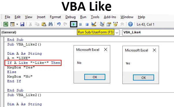
VBA Like используется, когда у нас есть некоторые специальные символы, пробелы в строке, и нам нужно получить точный или наиболее релевантный вывод этого слова. VBA Like позволяет сопоставлять шаблон в алфавитном порядке, так что если любое слово содержит некоторые специальные символы, то с помощью VBA Like мы можем завершить слово. Мы также можем определить, имеет ли эта строка правильный формат или нет.

В VBA Like у нас есть некоторые условия, на которых мы можем определить, что нам нужно получить и как нам нужно заполнить пространство пропущенных пустых слов.

• Вопросительный знак (?) — этим мы можем сопоставить только один символ из строки. Предположим, у нас есть строка «TAT» и шаблон «T? T», тогда VBA Like вернет TRUE. Если у нас есть строка «TOILET» и шаблон по-прежнему «T? T», тогда VBA Like вернет FALSE.
• Звездочка (*) — этим мы можем сопоставить 0 или более символов. Предположим, у нас есть строка «L ** K», тогда VBA Like вернет TRUE.
• (Char-Char) — этим мы можем сопоставить любой отдельный символ в диапазоне Char-Char.
• (! Char) — этим мы можем сопоставить любой отдельный символ, но не в списке.
• (! Char-Char) — этим мы можем сопоставить любой отдельный символ, но не в Char-Char.

Как использовать функцию VBA Like в Excel?

Мы научимся использовать функцию VBA Like на нескольких примерах в Excel.

Вы можете скачать этот шаблон VBA Like Excel здесь — Шаблон VBA Like Excel

Пример №1 — VBA Like

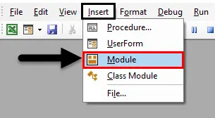
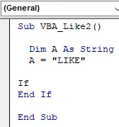
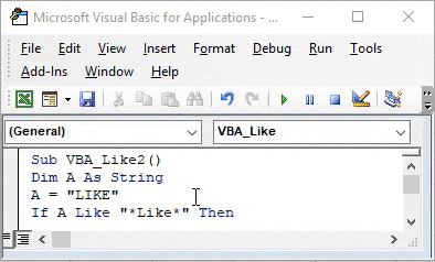
Чтобы узнать, является ли доступная строка ИСТИНА или ЛОЖЬ для VBA Как и прежде всего, нам нужен модуль. Для этого,

Шаг 1: Перейдите в меню « Вставка» и выберите « Модуль» из списка, как показано ниже.

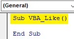
Шаг 2: Теперь в открывшемся окне Module в VBA напишите подкатегорию VBA Like, как показано ниже.

Код:

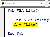
 Sub VBA_Like () End Sub 

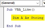
Шаг 3: Теперь сначала мы определим переменную A как String, как показано ниже. Здесь мы можем использовать переменную Long, так как она также позволяет хранить в ней любое текстовое значение.

Код:

 Sub VBA_Like () Dim A As String End Sub 

Шаг 4: Далее мы назначим слово переменной A. Давайте рассмотрим это слово как «LIKE».

Код:

 Sub VBA_Like () Dim A As String A = "Like" End Sub 

Шаг 5: Теперь с помощью цикла If-End If мы создадим условие VBA Like.

Код:

 Sub VBA_Like () Dim A As String A = "Like", если End End End End 

Мы будем использовать приведенный выше код и в следующем примере напрямую.

Шаг 6: Теперь в цикле If-End If записать условие как переменную A, например «L? KE», является ИСТИННЫМ условием, а затем дать нам « Да» в окне сообщения или же « Нет» в окне сообщения для ЛОЖЬ .

Код:

 Sub VBA_Like () Dim A As String A = "Like" Если A Like "L? KE", то MsgBox "Yes" Else MsgBox "No" End If End Sub 

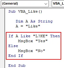
Мы сохранили знак вопроса на второй позиции. Но это может быть сохранено где угодно в целой строке.

Шаг 7: Теперь скомпилируйте код и запустите его, нажав кнопку Play, которая доступна под строкой меню.

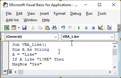
Мы получим окно сообщения как НЕТ. Это означает, что слово, выбравшее «LIKE» в переменной A, может иметь другие алфавиты вместо знака вопроса и вместо «I».

Пример № 2 — VBA Like

В этом примере мы будем реализовывать Asterisk (*)

Шаг 1: Теперь мы будем использовать ту же структуру кода, которую мы видели в примере 1, с тем же словом « LIKE ».

Код:

 Sub VBA_Like2 () Dim A As String A = "LIKE" If End If End Sub 

Шаг 2: Поскольку мы знаем, что с Asterisk у нас есть совпадение 0 или более символов из любой строки. Таким образом, в цикле If-End If мы напишем: если VBA Like соответствует «* Like *», это TRUE, тогда мы получим сообщение как Yes, иначе мы получим No, если это FALSE .

Код:

 Sub VBA_Like2 () Dim A As String A = "LIKE" Если A Like "* Like *", то MsgBox "Yes" Else MsgBox "No" End If End Sub 

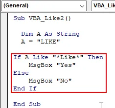
Шаг 3: Снова скомпилируйте полный код и запустите его. Мы получим сообщение как НЕТ, потому что VBA Like не соответствует ни одному алфавиту, кроме определенной строки « Like ».

Шаг 4: Теперь, если мы изменим строку A с «Like» на «Like Wise» и попытаемся сопоставить любую букву из строки, скажем, это «W» в звездочке, тогда что мы получим?

Как сказано выше, мы использовали «LIKE WISE» в качестве нашей новой строки.

Код:

 Sub VBA_Like2 () Dim A As String A = "LIKE WISE" Если A Like "* W *", то MsgBox "Да", иначе MsgBox "Нет" End If End Sub 

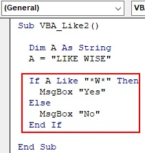
Шаг 5: Теперь скомпилируйте код и запустите его снова. Мы получим сообщение как ДА. Это означает, что VBA Like может соответствовать любому алфавиту из нашей строки «LIKE WISE».

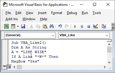
Таким же образом, если мы сопоставим любое другое письмо от «LIKE WISE», мы можем получить те же результаты.

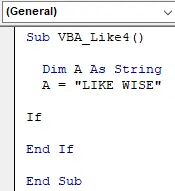
Пример № 3 — VBA Like

В этом примере мы увидим, как Char-Char работает в сопоставлении строк символов.

Шаг 1: Для этого мы также будем использовать тот же кадр кода, который мы видели в примере 2 для определенной переменной A как «LIKE WISE».

Код:

 Sub VBA_Like4 () Dim A As String A = "LIKE WISE" If End If End Sub 

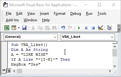
Шаг 2: В цикле if-End If напишите условие VBA Like, совпадающее с буквами от I до K ( в Asterisk и Char ), тогда оно будет TRUE и даст нам сообщение как YES . Если нет, то это будет ЛОЖЬ, и мы получим сообщение как НЕТ .

Код:

 Sub VBA_Like4 () Dim A As String A = "LIKE WISE" Если A Like "* (IK) *" Тогда MsgBox "Да" Иначе MsgBox "Нет" End If End Sub 

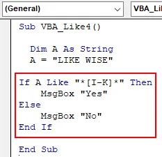
Шаг 3: Снова скомпилируйте код и запустите его. Мы увидим, что VBA Like способен сопоставлять символы от буквы I до K и дал нам сообщение как YES .

Плюсы и минусы VBA Like

• В наборе баз данных, где такие специальные символы встречаются довольно часто, использование VBA Like позволит нам создавать скрытые слова.
• Поскольку он имеет очень ограниченное применение, поэтому он очень редко используется.

То, что нужно запомнить

• Мы можем сравнивать и сопоставлять только строки. Любые другие переменные, такие как целые числа, нельзя использовать double.
• Не рекомендуется записывать макрос на VBA Like. Поскольку мы не знаем никакой функции Excel на нем. Кроме того, выполнение этого процесса другими способами может привести к получению неверных результатов матча.
• Хотя VBA Like используется очень редко, но вид вывода, который он выдает, может быть не совсем точно задан другими функциями и командами того же типа.
• Сохранить файл в макросе Включить только формат файла Excel. Этот формат в основном используется при создании любого макроса.

Рекомендуемые статьи

Это руководство к VBA Like. Здесь мы обсудим, как использовать функцию Excel VBA Like вместе с практическими примерами и загружаемым шаблоном Excel. Вы также можете просмотреть наши другие предлагаемые статьи —

1. VBA InStr объяснил с помощью примеров
2. Целочисленный тип данных VBA
3. Как выбрать ячейку, используя код VBA?
4. Транспонировать диапазон в VBA

I work as a data analyst in a clinic and we’re currently working on determining how many patients saw their assigned provider at their last visit. I typically run the reports and then export them to Excel for easier filtering. Previously, I was using a report that showed all the visit information along with RenderingProviderID and PrimaryCareProviderID, the former being the provider that actually saw the patient during the visit and the latter being the provider the patient was actually assigned to. It was easy to just add a column containing a formula to just look and see whether the IDs matched and then show a flag if they didn’t.

Now I’m using a different table where, instead of provider IDs, the result columns use their names. Better yet, the new Rendering Provider field just displays the last name while the PCP field shows full name and credentials. Results end up looking like this:

Visit ID      Rendering Provider      Primary Care Provider
---------------------------------------------------------------
00001         Smith                   Smith, John MD
00002         Smith                   Doe, Jane MD

Is there a formula I can use to find partial text matches in those two columns? I know what I want/need to do but I don’t know the syntax. I used to just add an extra column containing some form of IF statement and copy the formula all the way down — I’d usually just write it to leave the row blank for any matches and then display some sort of text for cases like the second example above where the RP and PCP didn’t match.

borro Пользователь Сообщений: 198 Регистрация: 01.01.1970	Здравствуйте! Потребовалось в ячейку вставить функцию, которая бы определяла соответствует ли ячейка,скажем, слева от неё шаблону, который используется для оператора like в VBA. Но не нашел, что написать. Например надо в столбце значений найти все ФИО, которые соответствуют шаблону «*  ?. ?.» для оператора like. Есть ли такая стандартная функция в Excel 2016?

	ПОИСК Даже самый простой вопрос можно превратить в огромную проблему. Достаточно не уметь формулировать вопросы…

borro Пользователь Сообщений: 198 Регистрация: 01.01.1970	Простите, вот пример значений

borro Пользователь Сообщений: 198 Регистрация: 01.01.1970

borro Пользователь Сообщений: 198 Регистрация: 01.01.1970	А для этой задачи ПОИСК уже не подойдёт? В этой задаче нужна чувствительность к регистру, к его смене.

vikttur Пользователь Сообщений: 47199 Регистрация: 15.09.2012

borro Пользователь Сообщений: 198 Регистрация: 01.01.1970	vikttur, НАЙТИ не учитывает подстановочные знаки при поиске

ответ элементарно НАЙТИ, если искать ответ, а не строчить вопросы в форумы реально, сомнительно какой метод эффективнее по времени: ждать пока кто-то ответит или настойчиво искать ответ самому думаете все, кто тут отвечает уже родились, знания ответы на эти вопросы? или может быть думаете, что я не пользуюсь поиском при ответах на некоторые вопросы? Программисты — это люди, решающие проблемы, о существовании которых Вы не подозревали, методами, которых Вы не понимаете!

Сергей Пользователь Сообщений: 11251 Регистрация: 01.01.1970	borro, а каким подстановочным знаком вы определяете регистр Лень двигатель прогресса, доказано!!!

Jack Famous Пользователь Сообщений: 10846 Регистрация: 07.11.2014 OS: Win 8.1 Корп. x64 | Excel 2016 x64: | Browser: Chrome

#11 20.03.2019 17:03:46 borro, макрофункция из приёмов Код Function MaskCompare(txt As String, mask As String, CaseSensitive As Boolean) If Not CaseSensitive Then txt = UCase$(txt): mask = UCase$(mask) If txt Like mask Then MaskCompare = True End Function P.S: не увидел, что нужен аналог из штатных, но пусть уж будет… Изменено: Jack Famous — 20.03.2019 17:10:24 Во всех делах очень полезно периодически ставить знак вопроса к тому, что вы с давних пор считали не требующим доказательств (Бертран Рассел) ►Благодарности сюда◄

borro Пользователь Сообщений: 198 Регистрация: 01.01.1970	Сергей, для like есть возможность поймать смену регистра с помощью шаблона вида «*[а-яё][А-ЯЁ].*», что и хотелось бы применить с помощью пользовательских функций, не прибегая к VBA

_Boroda_ Пользователь Сообщений: 1496 Регистрация: 27.07.2013 Контакты см. в профиле	#13 20.03.2019 17:29:02 Хороший вопрос, но плохой файл-пример В примере нужно 4 Вами заполненных столбца — Где_ищем Что_ищем Требуемый_результат Пояснение_к_результату И побольше вариантов, не три, два из которых по сути одинаковы, а штук 20 хотя бы Скажи мне, кудесник, любимец ба’гов…

Author: Oscar Cronquist Article last updated on February 07, 2023

The LIKE operator allows you to match a string to a pattern using Excel VBA. The image above demonstrates a macro that uses the LIKE operator to match a string to a given pattern.

The pattern is built on specific characters that I will demonstrate below.

Excel VBA Function Syntax

result = string Like pattern

Arguments

result	Required. Any number.
string	Required. A string.
pattern	Required. A string that meets the required pattern characters described below.

1. What characters can you use as a pattern in the LIKE operator?

The following characters are specifically designed to assist you in building a pattern:

Character	Desc	Text
?	question mark	Matches any single character.
*	asterisk	Matches zero or more characters.
#	number or hash sign	Any single digit.

A1A* — You can also use a string combined with the characters above to build a pattern. This matches a string beginning with A1A or is equal to A1A. The asterisk matches zero characters as well.

Characters	Desc	Text
[abc]	brackets	Characters enclosed in brackets allow you to match any single character in the string.
[!abc]	exclamation mark	The exclamation mark (!)  matches any single character not in the string.
[A-Z]	hyphen	The hyphen lets you specify a range of characters.

Back to top

1.1 How to make the LIKE operator case insensitive?

Add Option compare binary or Option compare text before any macros or custom functions in your code module to change how string evaluations are made.

The default setting is Option compare binary. Use Option compare text to make the comparison case-insensitive but put the code in a separate module so other macros/functions are not affected.

Setting	Desc
Option compare binary	Default.
Option compare text	Case-insensitive evaluations.

To learn more, read this article: Option Compare Statement

Back to top

1.2 What does the LIKE operator return?

The image above shows a macro in the Visual Basic Editor that returns either TRUE or FALSE depending on if the pattern matches the string or not.

Pattern *1* matches 552513256 and the macro above shows a message box containing value True.

result = string Like pattern

The LIKE operator returns a boolean value, TRUE or FALSE depending on if the pattern is a match or not. You can save the boolean value to a variable, the line above stores the boolean value in the variable result.

Back to top

2. Compare a cell value to a pattern

This simple User Defined Function (UDF) lets you specify a pattern and compare it to a cell value. If there is a match, the function returns TRUE. If not, FALSE. I am going to use this UDF in the examples below.

'Name User Defined Function
'Parameter c declared data type Range
'Parameter pttrn declared data type String
Function Compare(c As Range, pttrn As String) As Boolean

'Evaluate string in variable c with pattern saved to variable pttrn
'Return the result to the User Defined Function
Compare = c Like pttrn
End Function

Copy the code above and paste it to a code module in the VB Editor, if you want to use it. Where to put the code?

We are going to use this User Defined Function to compare patterns with strings located on a worksheet, read the next section.

Back to top

2.1 How to use the question mark (?) character

The picture above demonstrates the User Defined Function we created in section 2. It takes the string in column B and compares it to the pattern in column D. A boolean value True or False is returned to column E.

UDF syntax: Compare(string, pattern)

A question mark (?) matches any single character.

Formula in cell E6:

=Compare(B6, D6)

Value in cell B6 ABC matches A?C specified in cell D6, TRUE is returned to cell E6.

Formula in cell E7:

=Compare(B7, D7)

Value in cell B7 ABCD does not match pattern A?D. BC are two characters, a question mark matches any single character. FALSE is returned in cell E3.

Formula in cell E8:

=Compare(B8, D8)

Value in cell B8 ABCD matches the pattern specified in cell D8, ?BC?. TRUE is returned to cell E8.

Back to top

2.2 How to use the asterisk (*) character

The image above demonstrates the User Defined Function (UDF) described in section 2, it evaluates if a pattern matches a string using the LIKE operator. If so returns True. If not, False.

The UDF is entered in cell E9, E10, and E11. The first argument in the Compare UDF is a cell reference to the string and the second argument is a cell reference to the pattern.

Let’s begin with the formula in cell E9:

=Compare(B9, D9)

The pattern tells you that the first three characters must be AAA and then the * (asterisk) matches zero or more characters. AAAC is a match to pattern AAA* and the UDF returns TRUE in cell E9.

Formula in cell E10:

=Compare(B10, D10)

aaa* does not match pattern AAAC. aaa is not equal to AAA. LIKE operator is case sensitive unless you change settings to Option Compare Text.

Formula in cell E11:

=Compare(B10, D10)

(*) matches zero or more characters, DDC23E matches DD*E.

Back to top

2.3 How to use the number sign or hashtag (#) character

The image above shows  patterns in column D and strings in column B, the hashtag character # matches a single digit. To match multiple digits use multiple #.

Formula in cell E3:

=Compare(B3, D3)

String 123 in cell B3 matches pattern 12#, TRUE is returned in cell E3.

Formula in cell E4:

=Compare(B4, D4)

String 123 in cell B4 does not match pattern 1# in cell D4, the hashtag character matches any single digit only.

Formula in cell E5:

=Compare(B5, D5)

String 123 in cell B5 matches the pattern in cell D5 #2#.

Back to top

2.4 Combining pattern characters

The following three examples use asterisks, question marks, and number signs combined.

Formula in cell E12:

=Compare(B12, D12)

Pattern *##?? in cell D12 matches string AA23BB in cell B12, the formula returns True in cell E12. The asterisk matches 0 (zero) to any number of characters, the hashtag matches any single digit.

Note that there are two hashtags in the pattern. The ? question mark matches any single character.

Formula in cell E13:

=Compare(B13, D13)

The string in cell B13 AA23BB does not match pattern *##? specified in cell D13. There must be one character after the digits, the string has two characters after the digits.

Formula in cell E14:

=Compare(B13, D13)

The string AA23BB in cell B14 matches the pattern in cell D14 *##*. The asterisk matches 0 (zero) to any number of characters, the hashtags match two single digits and the last pattern character is the asterisk.

Back to top

2.5 How to use brackets with the LIKE operator

Brackets match any single character you specify. A hyphen lets you compare a range of letters, however, they must be sorted from A to Z. [A-C] is a valid range but [C-A] is not valid.

Formula in cell E15:

=Compare(B15, D15)

The formula in cell E15 evaluates the string ABCD to pattern [A]* and returns TRUE. The first character in the string must be A or a, the number of remaining characters can be zero or any number in length.

Formula in cell E16:

=Compare(B16, D16)

The formula in cell E16 evaluates the string ABCD to pattern [A] and returns FALSE. The string must be only one character and that character must be A or a.

Formula in cell E17:

=Compare(B17, D17)

The formula in cell E17 compares the string ABCD to pattern [!A]* and returns FALSE. The first character in the string must be anything but character A and the number of remaining characters can be 0 (zero) or any number in length.

Formula in cell E18:

=Compare(B18, D18)

The formula in cell E18 compares the string C22R to pattern [A-Z]##? and returns TRUE. The first character in the string must be a letter between A to Z, then any two digits, and lastly a question mark that matches any single character.

Formula in cell E19:

=Compare(B19, D19)

The formula in cell E19 compares the string C22R to pattern [A-Z]##[A-Z] and returns TRUE. The string begins with any letter between A to Z, then any two digits, and lastly, any letter between A to Z.

Formula in cell E20:

=Compare(B20, D20)

The formula in cell E20 compares the string C222 to pattern [A-Z]##[A-Z] and returns FALSE. The string begins with any letter between A to Z, then any two digits, and lastly, any letter between A to Z. The string has a digit as the last character which isn’t a match.

Back to top

3. Search for a regex pattern in column and get matching values (UDF)

The following user-defined function allows you to extract cell values using the LIKE operator and a pattern specified on the worksheet.

The formula is entered in cell D6 as an array formula, it returns multiple values to cells below if the pattern matches multiple values.

The example pattern used is in cell D3 «?B?». The question mark matches a single character, the UDF returns all values containing three letters and the middle letter is B.

Array formula in cell D6:D9:

=SearchPattern(B3:B16, D3)

How to enter an array formula

'Name User-defined Function
Function SearchPattern(c As Range, pttrn As String)

'Dimension variables and declare data types
Dim d as String

'Iterate through each cell in c
For Each cell In c

'Check if string matches pttrn, if so concatenate cell value and comma to variable d
If cell Like pttrn Then d = d & cell & ","

'Continue with next cell
Next cell

'Split string in variable d using comma character then transpose array and return values to UDF SearchPattern
SearchPattern = Application.Transpose(Split(d, ","))
End Function

Where to put the code?

Back to top

4. Search for a pattern and return values in an adjacent column (UDF)

This User Defined Function allows you to look for a pattern in a column and return the corresponding value in another column.

The UDF returns a value from column C if the corresponding value in column B on the same row matches the regex pattern specified in cell E3.

Array formula in cell E6:E9:

=SearchCol(B3:B16, C3:C16, E3)

How to enter an array formula

'Name User Defined Function (UDF)
Function SearchCol(b As Range, c As Range, pttrn As String)

'Dimension variables and declare data types
Dim a As Long, d as String

'Count cells in cell range b
a = b.Cells.CountLarge

'For ... Next statement meaning iterate lines in between a times
For i = 1 To a

'Check if cell matches pattern, if so add c and a comma to variable d
If b.Cells(i) Like pttrn Then d = d & c.Cells(i) & ","
Next i

'Split values in variable d and return array to worksheet
SearchCol = Application.Transpose(Split(d, ","))
End Function

Where to put the code?

Back to top

5. Extract words that match a regex pattern from cell range (UDF)

The image above demonstrates a User Defined Function (UDF) that extracts words that match a given regex pattern. This means that the UDF may extract multiple words from the same cell.

You can use this UDF to extract phone numbers, zip codes, email addresses, html code, or pretty much anything from cells that contain a lot of data.

Array formula in cell D5:

=ExtractWords(B3:B10,E2)

If you want to split the data using a different character change the space character in the VBA code below to any delimiting character or characters.

5.1 How to enter an array formula

1. Select the cell range you want to use.
2. Press with left mouse button on in the formula bar.
3. Paste array formula to the formula bar.
4. Press and hold CTRL + SHIFT simultaneously.
5. Press Enter once.
6. Release all keys.

Your formula is now an array formula, you recognize array formulas by the beginning and ending curly brackets in the formula bar. {=array_formula}

Don’t enter these characters yourself, they appear automatically.

5.2 VBA code

'Name User Defined Function (UDF)
Function ExtractWords(c As Range, pttrn As String)

'Iterate through each cell in cell range c
For Each cell In c

    'Split cell contents into an array using space as a delimiting character
    Arr = Split(cell, " ")

    'Iterate through each value in array Arr
    For Each a In Arr

        'Check if string in variable a matches pattern in variable pttrn
        If a Like pttrn Then

            'Add string a and a comma to variable d
            d = d & a & ","
        End If
    Next
    
Next cell

'Split variable d using comma as a delimiting character and return array to UDF
ExtractWords = Application.Transpose(Split(d, ","))

End Function

6. Where to put the code?

1. Press Alt+F11 to open the Visual Basic Editor (VBE).
2. Press with mouse on «Insert» on the top menu, see image above.
3. A popup menu appears. Press with left mouse button on «Module» to insert a module to your workbook.
4. Copy the VBA code.
5. Paste to the code window.
6. Return to Excel.

Note, save your workbook with file extension *.xlsm (macro-enabled workbook) to attach the code. This step is important.

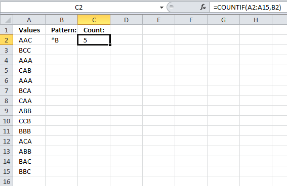
Did you know?

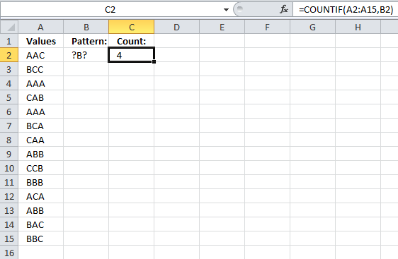
You can use the question (?)  mark and asterisk (*) characters in many Excel functions. The COUNTIF function in cell C2 demonstrated in the image above counts cells in cell range A2:A15 using the pattern in cell B2.

If you need to use even more complicated patterns Excel allows you to use regular expressions, see this thread:
How to use Regular Expressions (Regex) in Microsoft Excel both in-cell and loops

Back to top

Back to top