Overview of formulas in Excel
Get started on how to create formulas and use built-in functions to perform calculations and solve problems.
Important: The calculated results of formulas and some Excel worksheet functions may differ slightly between a Windows PC using x86 or x86-64 architecture and a Windows RT PC using ARM architecture. Learn more about the differences.
Important: In this article we discuss XLOOKUP and VLOOKUP, which are similar. Try using the new XLOOKUP function, an improved version of VLOOKUP that works in any direction and returns exact matches by default, making it easier and more convenient to use than its predecessor.
Create a formula that refers to values in other cells
-
Select a cell.
-
Type the equal sign =.
Note: Formulas in Excel always begin with the equal sign.
-
Select a cell or type its address in the selected cell.
-
Enter an operator. For example, – for subtraction.
-
Select the next cell, or type its address in the selected cell.
-
Press Enter. The result of the calculation appears in the cell with the formula.
See a formula
-
When a formula is entered into a cell, it also appears in the Formula bar.
-
To see a formula, select a cell, and it will appear in the formula bar.
Enter a formula that contains a built-in function
-
Select an empty cell.
-
Type an equal sign = and then type a function. For example, =SUM for getting the total sales.
-
Type an opening parenthesis (.
-
Select the range of cells, and then type a closing parenthesis).
-
Press Enter to get the result.
Download our Formulas tutorial workbook
We’ve put together a Get started with Formulas workbook that you can download. If you’re new to Excel, or even if you have some experience with it, you can walk through Excel’s most common formulas in this tour. With real-world examples and helpful visuals, you’ll be able to Sum, Count, Average, and Vlookup like a pro.
Formulas in-depth
You can browse through the individual sections below to learn more about specific formula elements.
A formula can also contain any or all of the following: functions, references, operators, and constants.
Parts of a formula
1. Functions: The PI() function returns the value of pi: 3.142…
2. References: A2 returns the value in cell A2.
3. Constants: Numbers or text values entered directly into a formula, such as 2.
4. Operators: The ^ (caret) operator raises a number to a power, and the * (asterisk) operator multiplies numbers.
A constant is a value that is not calculated; it always stays the same. For example, the date 10/9/2008, the number 210, and the text «Quarterly Earnings» are all constants. An expression or a value resulting from an expression is not a constant. If you use constants in a formula instead of references to cells (for example, =30+70+110), the result changes only if you modify the formula. In general, it’s best to place constants in individual cells where they can be easily changed if needed, then reference those cells in formulas.
A reference identifies a cell or a range of cells on a worksheet, and tells Excel where to look for the values or data you want to use in a formula. You can use references to use data contained in different parts of a worksheet in one formula or use the value from one cell in several formulas. You can also refer to cells on other sheets in the same workbook, and to other workbooks. References to cells in other workbooks are called links or external references.
-
The A1 reference style
By default, Excel uses the A1 reference style, which refers to columns with letters (A through XFD, for a total of 16,384 columns) and refers to rows with numbers (1 through 1,048,576). These letters and numbers are called row and column headings. To refer to a cell, enter the column letter followed by the row number. For example, B2 refers to the cell at the intersection of column B and row 2.
To refer to
Use
The cell in column A and row 10
A10
The range of cells in column A and rows 10 through 20
A10:A20
The range of cells in row 15 and columns B through E
B15:E15
All cells in row 5
5:5
All cells in rows 5 through 10
5:10
All cells in column H
H:H
All cells in columns H through J
H:J
The range of cells in columns A through E and rows 10 through 20
A10:E20
-
Making a reference to a cell or a range of cells on another worksheet in the same workbook
In the following example, the AVERAGE function calculates the average value for the range B1:B10 on the worksheet named Marketing in the same workbook.
1. Refers to the worksheet named Marketing
2. Refers to the range of cells from B1 to B10
3. The exclamation point (!) Separates the worksheet reference from the cell range reference
Note: If the referenced worksheet has spaces or numbers in it, then you need to add apostrophes (‘) before and after the worksheet name, like =’123′!A1 or =’January Revenue’!A1.
-
The difference between absolute, relative and mixed references
-
Relative references A relative cell reference in a formula, such as A1, is based on the relative position of the cell that contains the formula and the cell the reference refers to. If the position of the cell that contains the formula changes, the reference is changed. If you copy or fill the formula across rows or down columns, the reference automatically adjusts. By default, new formulas use relative references. For example, if you copy or fill a relative reference in cell B2 to cell B3, it automatically adjusts from =A1 to =A2.
Copied formula with relative reference
-
Absolute references An absolute cell reference in a formula, such as $A$1, always refer to a cell in a specific location. If the position of the cell that contains the formula changes, the absolute reference remains the same. If you copy or fill the formula across rows or down columns, the absolute reference does not adjust. By default, new formulas use relative references, so you may need to switch them to absolute references. For example, if you copy or fill an absolute reference in cell B2 to cell B3, it stays the same in both cells: =$A$1.
Copied formula with absolute reference
-
Mixed references A mixed reference has either an absolute column and relative row, or absolute row and relative column. An absolute column reference takes the form $A1, $B1, and so on. An absolute row reference takes the form A$1, B$1, and so on. If the position of the cell that contains the formula changes, the relative reference is changed, and the absolute reference does not change. If you copy or fill the formula across rows or down columns, the relative reference automatically adjusts, and the absolute reference does not adjust. For example, if you copy or fill a mixed reference from cell A2 to B3, it adjusts from =A$1 to =B$1.
Copied formula with mixed reference
-
-
The 3-D reference style
Conveniently referencing multiple worksheets If you want to analyze data in the same cell or range of cells on multiple worksheets within a workbook, use a 3-D reference. A 3-D reference includes the cell or range reference, preceded by a range of worksheet names. Excel uses any worksheets stored between the starting and ending names of the reference. For example, =SUM(Sheet2:Sheet13!B5) adds all the values contained in cell B5 on all the worksheets between and including Sheet 2 and Sheet 13.
-
You can use 3-D references to refer to cells on other sheets, to define names, and to create formulas by using the following functions: SUM, AVERAGE, AVERAGEA, COUNT, COUNTA, MAX, MAXA, MIN, MINA, PRODUCT, STDEV.P, STDEV.S, STDEVA, STDEVPA, VAR.P, VAR.S, VARA, and VARPA.
-
3-D references cannot be used in array formulas.
-
3-D references cannot be used with the intersection operator (a single space) or in formulas that use implicit intersection.
What occurs when you move, copy, insert, or delete worksheets The following examples explain what happens when you move, copy, insert, or delete worksheets that are included in a 3-D reference. The examples use the formula =SUM(Sheet2:Sheet6!A2:A5) to add cells A2 through A5 on worksheets 2 through 6.
-
Insert or copy If you insert or copy sheets between Sheet2 and Sheet6 (the endpoints in this example), Excel includes all values in cells A2 through A5 from the added sheets in the calculations.
-
Delete If you delete sheets between Sheet2 and Sheet6, Excel removes their values from the calculation.
-
Move If you move sheets from between Sheet2 and Sheet6 to a location outside the referenced sheet range, Excel removes their values from the calculation.
-
Move an endpoint If you move Sheet2 or Sheet6 to another location in the same workbook, Excel adjusts the calculation to accommodate the new range of sheets between them.
-
Delete an endpoint If you delete Sheet2 or Sheet6, Excel adjusts the calculation to accommodate the range of sheets between them.
-
-
The R1C1 reference style
You can also use a reference style where both the rows and the columns on the worksheet are numbered. The R1C1 reference style is useful for computing row and column positions in macros. In the R1C1 style, Excel indicates the location of a cell with an «R» followed by a row number and a «C» followed by a column number.
Reference
Meaning
R[-2]C
A relative reference to the cell two rows up and in the same column
R[2]C[2]
A relative reference to the cell two rows down and two columns to the right
R2C2
An absolute reference to the cell in the second row and in the second column
R[-1]
A relative reference to the entire row above the active cell
R
An absolute reference to the current row
When you record a macro, Excel records some commands by using the R1C1 reference style. For example, if you record a command, such as clicking the AutoSum button to insert a formula that adds a range of cells, Excel records the formula by using R1C1 style, not A1 style, references.
You can turn the R1C1 reference style on or off by setting or clearing the R1C1 reference style check box under the Working with formulas section in the Formulas category of the Options dialog box. To display this dialog box, click the File tab.
Top of Page
Need more help?
You can always ask an expert in the Excel Tech Community or get support in the Answers community.
See Also
Switch between relative, absolute and mixed references for functions
Using calculation operators in Excel formulas
The order in which Excel performs operations in formulas
Using functions and nested functions in Excel formulas
Define and use names in formulas
Guidelines and examples of array formulas
Delete or remove a formula
How to avoid broken formulas
Find and correct errors in formulas
Excel keyboard shortcuts and function keys
Excel functions (by category)
Need more help?
This post will guide you how to convert a string into a formula in Excel. How do I turn test strings to a formula for calculation.
Assuming that you have a list of data in range C1:C4, which contains text string (Actually, they are all formulas, but they are shown as text string format), and you want to convert those test string into a formula for calculation. How to do it. You can create your own Excel Functions with VBA Code. It is also called as a User Defined Function. And it work the same way as Excel’s build-in standard functions. Just do the following steps:
#1 open your excel workbook and then click on “Visual Basic” command under DEVELOPER Tab, or just press “ALT+F11” shortcut.
#2 then the “Visual Basic Editor” window will appear.
#3 click “Insert” ->”Module” to create a new module.
#4 paste the below VBA code into the code window. Then clicking “Save” button.
Function EvaluateString(strTextString As String)
     Application.Volatile
     EvaluateString = Evaluate(strTextString)
End Function
#5 back to the current worksheet, then type the following formula in a blank cell, and then press Enter key. And drag the AutoFill Handle over to other cells.
=EvaluateString(C1)
You would notice that all strings in range C1:C4 have been converted as formulas.
my initial problem was to extract all numbers except the first one from an equation and sum in another cell: A1: «=6+5+4». A2: «9». Maybe it can be solved without VBA?
You could try (assuming only addition):
Formula in B1:
=SUM(FILTERXML("<t><s>"&SUBSTITUTE(MID(A1,2,LEN(A1)),"+","</s><s>")&"</s></t>","//s[position()>1]"))
In fact, if you don’t want to use the 1st number we could also discard taking ‘=’ into account:
=SUM(FILTERXML("<t><s>"&SUBSTITUTE(A1,"+","</s><s>")&"</s></t>","//s[position()>1]"))
And since SUM() will ignore text in the final answer, we can now even further simplify this (thanks @JosWoolley):
=SUM(FILTERXML("<t><s>"&SUBSTITUTE(A1,"+","</s><s>")&"</s></t>","//s"))
How to Create a Formula in Excel: Beginner Tutorial (2023)
Excel is all about running calculations! And so creating and operating a formula in Excel is simple.
An Excel formula is a combination of operators and operands. For example, 2 + 2 = 4 is a formula where 2s are the operands, plus sign (+) is the operator, and 4 is the answer to the formula.
Only if you know the basics to write a formula in Excel – there’s a high chance you’d solve most of your Excel problems. This article explains the basics of creating Excel formulas.
So let’s dive right in.
As you scroll down, download our free sample workbook here to practice the examples used in the guide below. 😀
How to create formulas in Excel
Creating Excel formulas is easy as pie.
For example, what is 10 divided by 2? Can you calculate this in Excel?
1. Start by activating a cell.
2. Write an equal sign.

It is very important to start any formula with an equal sign. If you do not start with an equal sign, Excel wouldn’t recognize it as a formula but as a text string.
3. Input the simple mathematical operation of 10 divided by 2.
= 10 / 2

4. Hit enter, and you’re good to go!

You can create the same above formula with a slight variation.
For example, if you have the operands as cell values.

1. Write the formula using cell references as follows.
= A2 / B2

The above formula translates to ‘A2 divided by A3’.
Where A2 has the numeric value 10, and A3 has the numeric value 2.
2. The results remain the same as in the above example.

Creating a formula using cell references and values
The same formula can also be created using a combination of cell references and values.
Write the following formula using cell references and values.
= A2 / 2

The above formula translates to ‘A2 divided by 2’.
Where A2 has the numeric value 10, and 2 is a value.
1. The results look as follows.

Pro Tip!
Using cell references is better than using absolute values. This is because if sometime later you change the cell value – the formula would automatically update.
How to add, subtract, multiply, and divide?
There are four basic mathematical operations – add, subtract, multiply, and divide.
Let’s now see how to perform each of these operations in Excel.
How to make a SUM formula (addition)
Adding things up in Excel can take different forms.
Excel has an in-built function for performing addition i.e. the SUM function. Here’s how you can bring it to action.
1. Write the SUM function beginning with an equal sign as follows.
= SUM (5, 5)
Every argument of the SUM function separated by a comma represents the value to be added.
Excel adds 5 into 5 to give the results below.

Easy enough? You can use the SUM function for cell references too. 🤩
2. Write the SUM function as follows.
= SUM (A2, A3)
Pro Tip!
To insert SUM from the Insert Function button, take this route.
Go to Formulas tab > Function Library > Insert function button > Type the function name.
In the Insert Function dialog box, type SUM and hit search. Select the desired function and hit ‘Okay’ to insert the same.
Excel adds the cell values of Cell A2 and Cell A3.

What makes the SUM function a big plus is its ability to add up a range of cells.
For example, see the data below.

3. To add this up in Excel using the SUM function, write the SUM function as below.
= SUM (A2:A10)

Must notice how we have defined the cell range from Cell A2 to Cell A10 as A2:A10.
4. Excel sums up all cell values in cells from A2 to A10.

You can make this function work even more interestingly by adding up multiple ranges.
5. Write the SUM function with multiple ranges as follows.
= SUM (A2:A5, B2:B8, C1:C10)


How to subtract in Excel
Subtracting in Excel is all about creating a formula with the minus sign operator (-).
For example:
1. To subtract 5 from 10, begin with an equal sign and write the following formula.
= 10 – 5
A simple subtraction formula with a minus sign operator!
Press enter and here you go.

2. Try doing the same with cell references as below.
= A2 – A3
This formula translates to A2 less A3. Where A2 has the numeric value 10, and A3 has the numeric value 5.

3. Alternatively, you can use the SUM function to perform subtraction. However, to do this you need to add a minus sign to the value to be subtracted.
= SUM (A2, -A3)
Here are the results.

How to multiply in Excel
After we have learned how to add and subtract in Excel, it’s time we learn multiplication in Excel.
First thing first, the operator for multiplication in Excel is an asterisk (*).
Now, do you remember what is 9 times 8? No?
1. Write a multiplication formula in Excel.
= 9 * 8


2. Try doing the same using cell references as below.
= A2 * A3

The formula above translates to A2 multiplied by A3.
Excel also offers an in-built function for multiplication in Excel. The PRODUCT Function!
3. Write the PRODUCT function as follows.
= PRODUCT (9, 

We have added both the values to be multiplied as the arguments to the PRODUCT function.
Here are the results.

The PRODUCT function can also find the product of multiple values (or a range of cells) at once.
For example, see the data below.

4. To multiply all these values, write the PRODUCT function as follows:
= PRODUCT (A2:A10)

Excel multiplies all the values in the specified range.

How to divide in Excel
Here comes the last operation of this guide – division. 🤞
Creating a division formula in Excel is also very straightforward.
What is the operator for division? A forward slash (/).
Also, the dividend (or the numerator) comes before the slash. And the divisor (or the denominator) comes after the slash.
1. Write a division formula as below.
= 30 / 10

Excel divides both operands to give the results as follows.

2. The same can be done using cell references.
= A2 / A3

Pro Tip!
While performing the division function in Excel, you might see the #DIV/0! Error. This error is given back by Excel when you attempt to divide the number of zero.
Basic Rule of Grade 6! No number is divisible by zero. Excel remembers that, if not us. 😆
Order of operations
Here’s an equation for you to solve.
= 2+ 4 * 6 / 3 – 2
What a mess! Which operation do you perform first?
To solve this mystery, there is an order for performing mathematical operations – PEMDAS
P = Parenthesis
E = Exponents
MD = Multiplication & Division (left to right)
AS = Addition & Subtraction
Solve the above equation in the same order, and you’d reach the answer 8.
Let Excel do the same to see the results.

Excel performs division first (6 / 3 = 2), multiplication second (4 * 2 = 8), addition third (2 + 8 = 10), and subtraction last (10 – 2 = 8), resulting in 8.
Now, let’s enclose a part of this formula in parentheses to see how the results change.
= 2+ 4 * 6 / (3 – 2)

What causes the results to change with only parenthesis added?
Excel now first performs the operation enclosed in parenthesis i.e. (3-2).
Next, multiplication is performed, then division and addition last. This causes the answer to change.
Pro Tip!
Try doing some mental maths to double-check if Excel has rightly calculated 26.
Parenthesis first = 2+ 4*6/(3 – 2)
Multiplication Second= 2+4*6/1
Division Third = 2 + 24/1
Addition Last = 2 + 24
Here’s the answer = 26
How to create formulas with references
Creating Excel formulas with references is super simple. All you need to do is replace the values in a simple formula with cell references (cells that contain those values).
For example, let’s create a multiplication formula in Excel.

Great! What if you had 2 & 4 as numerical values in cells?

Create the same formula using cell references.

You can do the same for all operators! It is this simple.
Also, what happens when a cell value changes? Until the cell reference is in place, the formula would automatically update for the cell value change.

Must note how the cell reference in the formula remains unchanged. The answer however changes as the cell value for A3 has changed.ltiple criteria lookup💡
Formulas or functions?
What is an Excel formula, and what is an Excel function? And how are these two different?
There are two ways to add 2 and 2 in Excel.
- = 2 + 2
- SUM (2,2)
The answer to them both would be the same. However, the first one is a formula created in Excel. Whereas the second one is an in-built function of Excel – the SUM function.
Functions are more like predefined formulas in Excel.
Although the function library of Microsoft Excel is huge enough for you to explore, there is a limit to it. And you may not find everything you need there.
So, you might still need to write your own formulas to perform calculations in Excel. 😉
Pro Tip!
Sometimes, you might even nest a function into a formula.
For example, what is 2 + 2 – 3?
You may write it as = (SUM (2,2)) – 3
SUM (2,2) is a function, and deducting 3 from it makes it a self-created formula.
That’s it – Now what?
Until now, we’ve created formulas using different operators, values, and cell references. And learned how to use the SUM function for addition and subtraction.
Not only that but we’ve also studied the order of operations in Excel. The above article is a whole pack of information, isn’t it?
Creating your own formulas in Excel is the first step to manipulating numbers in Excel. However, this is something very basic, and Excel has tons more to offer.
Some very important Excel functions that one must hone include the VLOOKUP, SUMIF, and IF functions.
Haven’t mastered them yet? Click here to register for my 30-minute free email course that helps you learn these and much more.
Kasper Langmann2023-02-23T14:38:38+00:00
Page load link
Enter a Formula | Edit a Formula | Operator Precedence | Copy/Paste a Formula | Insert Function
A formula is an expression which calculates the value of a cell. Functions are predefined formulas and are already available in Excel.
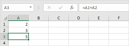
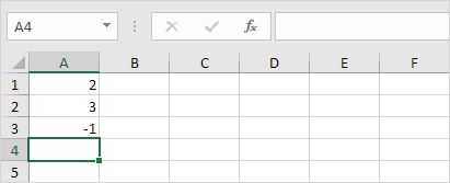
Cell A3 below contains a formula which adds the value of cell A2 to the value of cell A1.
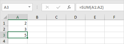
Cell A3 below contains the SUM function which calculates the sum of the range A1:A2.
Enter a Formula
To enter a formula, execute the following steps.
1. Select a cell.
2. To let Excel know that you want to enter a formula, type an equal sign (=).
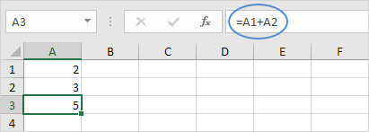
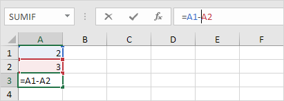
3. For example, type the formula A1+A2.
Tip: instead of typing A1 and A2, simply select cell A1 and cell A2.
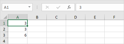
4. Change the value of cell A1 to 3.
Excel automatically recalculates the value of cell A3. This is one of Excel’s most powerful features!
Edit a Formula
When you select a cell, Excel shows the value or formula of the cell in the formula bar.
1. To edit a formula, click in the formula bar and change the formula.
2. Press Enter.
Operator Precedence
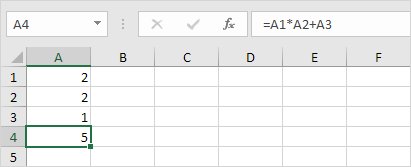
Excel uses a default order in which calculations occur. If a part of the formula is in parentheses, that part will be calculated first. It then performs multiplication or division calculations. Once this is complete, Excel will add and subtract the remainder of your formula. See the example below.
First, Excel performs multiplication (A1 * A2). Next, Excel adds the value of cell A3 to this result.
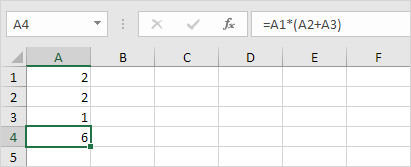
Another example,
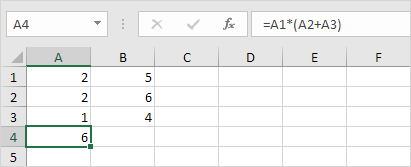
First, Excel calculates the part in parentheses (A2+A3). Next, it multiplies this result by the value of cell A1.
Copy/Paste a Formula
When you copy a formula, Excel automatically adjusts the cell references for each new cell the formula is copied to. To understand this, execute the following steps.
1. Enter the formula shown below into cell A4.
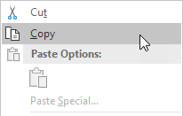
2a. Select cell A4, right click, and then click Copy (or press CTRL + c)…
…next, select cell B4, right click, and then click Paste under ‘Paste Options:’ (or press CTRL + v).
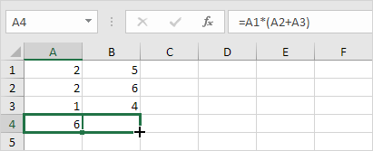
2b. You can also drag the formula to cell B4. Select cell A4, click on the lower right corner of cell A4 and drag it across to cell B4. This is much easier and gives the exact same result!
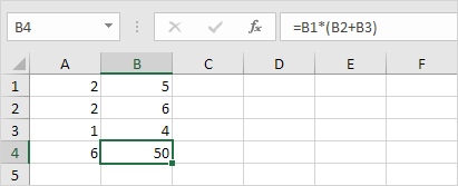
Result. The formula in cell B4 references the values in column B.
Insert Function
Every function has the same structure. For example, SUM(A1:A4). The name of this function is SUM. The part between the brackets (arguments) means we give Excel the range A1:A4 as input. This function adds the values in cells A1, A2, A3 and A4. It’s not easy to remember which function and which arguments to use for each task. Fortunately, the Insert Function feature in Excel helps you with this.
To insert a function, execute the following steps.
1. Select a cell.
2. Click the Insert Function button.
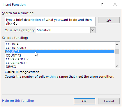
The ‘Insert Function’ dialog box appears.
3. Search for a function or select a function from a category. For example, choose COUNTIF from the Statistical category.
4. Click OK.
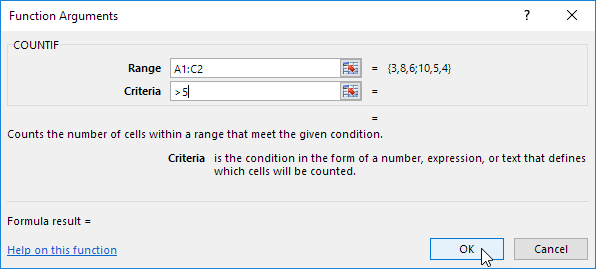
The ‘Function Arguments’ dialog box appears.
5. Click in the Range box and select the range A1:C2.
6. Click in the Criteria box and type >5.
7. Click OK.
Result. The COUNTIF function counts the number of cells that are greater than 5.
Note: instead of using the Insert Function feature, simply type =COUNTIF(A1:C2,»>5″). When you arrive at: =COUNTIF( instead of typing A1:C2, simply select the range A1:C2.


