
Excel for Microsoft 365 Excel for Microsoft 365 for Mac Excel for the web Excel 2021 Excel 2021 for Mac Excel 2019 Excel 2019 for Mac Excel 2016 Excel 2016 for Mac Excel 2013 Excel 2010 Excel for Mac 2011 Excel Mobile More…Less
Managing personal finances can be a challenge, especially when trying to plan your payments and savings. Excel formulas and budgeting templates can help you calculate the future value of your debts and investments, making it easier to figure out how long it will take for you to reach your goals. Use the following functions:
-
PMT calculates the payment for a loan based on constant payments and a constant interest rate.
-
NPER calculates the number of payment periods for an investment based on regular, constant payments and a constant interest rate.
-
PV returns the present value of an investment. The present value is the total amount that a series of future payments is worth now.
-
FV returns the future value of an investment based on periodic, constant payments and a constant interest rate.
Figure out the monthly payments to pay off a credit card debt
Assume that the balance due is $5,400 at a 17% annual interest rate. Nothing else will be purchased on the card while the debt is being paid off.
Using the function PMT(rate,NPER,PV)
=PMT(17%/12,2*12,5400)
the result is a monthly payment of $266.99 to pay the debt off in two years.
-
The rate argument is the interest rate per period for the loan. For example, in this formula the 17% annual interest rate is divided by 12, the number of months in a year.
-
The NPER argument of 2*12 is the total number of payment periods for the loan.
-
The PV or present value argument is 5400.
Figure out monthly mortgage payments
Imagine a $180,000 home at 5% interest, with a 30-year mortgage.
Using the function PMT(rate,NPER,PV)
=PMT(5%/12,30*12,180000)
the result is a monthly payment (not including insurance and taxes) of $966.28.
-
The rate argument is 5% divided by the 12 months in a year.
-
The NPER argument is 30*12 for a 30 year mortgage with 12 monthly payments made each year.
-
The PV argument is 180000 (the present value of the loan).
Find out how to save each month for a dream vacation
You’d like to save for a vacation three years from now that will cost $8,500. The annual interest rate for saving is 1.5%.
Using the function PMT(rate,NPER,PV,FV)
=PMT(1.5%/12,3*12,0,8500)
to save $8,500 in three years would require a savings of $230.99 each month for three years.
-
The rate argument is 1.5% divided by 12, the number of months in a year.
-
The NPER argument is 3*12 for twelve monthly payments over three years.
-
The PV (present value) is 0 because the account is starting from zero.
-
The FV (future value) that you want to save is $8,500.
Now imagine that you are saving for an $8,500 vacation over three years, and wonder how much you would need to deposit in your account to keep monthly savings at $175.00 per month. The PV function will calculate how much of a starting deposit will yield a future value.
Using the function PV(rate,NPER,PMT,FV)
=PV(1.5%/12,3*12,-175,8500)
an initial deposit of $1,969.62 would be required in order to be able to pay $175.00 per month and end up with $8500 in three years.
-
The rate argument is 1.5%/12.
-
The NPER argument is 3*12 (or twelve monthly payments for three years).
-
The PMT is -175 (you would pay $175 per month).
-
The FV (future value) is 8500.
Find out how long it will take to pay off a personal loan
Imagine that you have a $2,500 personal loan, and have agreed to pay $150 a month at 3% annual interest.
Using the function NPER(rate,PMT,PV)
=NPER(3%/12,-150,2500)
it would take 17 months and some days to pay off the loan.
-
The rate argument is 3%/12 monthly payments per year.
-
The PMT argument is -150.
-
The PV (present value) argument is 2500.
Figure out a down payment
Say that you’d like to buy a $19,000 car at a 2.9% interest rate over three years. You want to keep the monthly payments at $350 a month, so you need to figure out your down payment. In this formula the result of the PV function is the loan amount, which is then subtracted from the purchase price to get the down payment.
Using the function PV(rate,NPER,PMT)
=19000-PV(2.9%/12, 3*12,-350)
the down payment required would be $6,946.48
-
The $19,000 purchase price is listed first in the formula. The result of the PV function will be subtracted from the purchase price.
-
The rate argument is 2.9% divided by 12.
-
The NPER argument is 3*12 (or twelve monthly payments over three years).
-
The PMT is -350 (you would pay $350 per month).
See how much your savings will add up to over time
Starting with $500 in your account, how much will you have in 10 months if you deposit $200 a month at 1.5% interest?
Using the function FV(rate,NPER,PMT,PV)
=FV(1.5%/12,10,-200,-500)
in 10 months you would have $2,517.57 in savings.
-
The rate argument is 1.5%/12.
-
The NPER argument is 10 (months).
-
The PMT argument is -200.
-
The PV (present value) argument is -500.
See also
PMT function
NPER function
PV function
FV function
Need more help?
Want more options?
Explore subscription benefits, browse training courses, learn how to secure your device, and more.
Communities help you ask and answer questions, give feedback, and hear from experts with rich knowledge.
The effective rate of interest on the loan (as with almost on any other financial instrument) – this is the expression of all future cash payments (incomes from a financial instrument), which are included in the treaty provision of the contract, in the figure annual interest. That is the real interest that the debtor will pay for using of money in the Bank (investor – to obtain). Here is taken into account the rate of interest designated in the contract, all fees, repayment schemes, loan term (of deposit).
The calculation of the effective rate on the loan in Excel
There are the range of built-in functions in Excel, that allow you to compute the effective rate of interest, with taking into account additional charges and fees, and excluding (relying only on the nominal interest and the loan term).
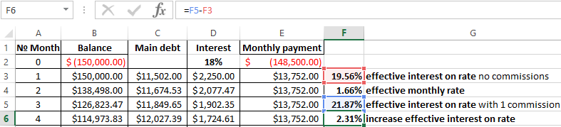
The debtor took a credit in the sum of 150 000$ on the term of 1 year (12 months). The nominal annual rate — is 18%. Payments on the loan specify in the table below:
Since this example does not include the additional fees and charges, we determine to the annual effective rate using the function EFFECT.
We are calling: «FORMULAS»-«Function Library»-«Financial» finding the function EFFECT. The arguments:
- «Nominal rate» — is the annual rate of interest on the credit, which is designated in the agreement with the Bank. In this example – is 18% (0, 18).
- «Number of periods» — the number of periods in a year, for which interests are charged. In this example – there are 12 months.
The effective interest on rate — is 19. 56%.
Let’s complicate the task by adding the one-time commission loan at the amount of 1% of the sum of 150 000$. In monetary terms – is 1500$. So, the borrower to get on his hands is the sum of 148 500$.
For calculating to the effective monthly rate, we need use the IRR function (return to the internal rate of return for cash flow):
We have made the column with monthly payments 148 500 with the sign «-», because the money the Bank first gives. Payments which the debtor will make in the cashier subsequently are positive for the bank. The internal rate of return we consider from the Bank’s point of view: it acts as an investor.
The function has given to the effective monthly rate of 1.6617121%. For the calculating of the nominal rate to the result need multiply by 12 (the term of loan): 1.662% * 12 = 19.94%. Let`s recalculate the effective interest percent:
The one-time fee in amount of 1% increased the actual annual interest on 2.31%. It was: 21, 87%.
We add in the scheme of payments on the loan to the monthly fee for account maintenance in the amount of 30$. Monthly effective rate will be equal to 1.6968%.
The nominal percent is 1.6968% * 12 = is 20.3616%. The effective annual rate is:
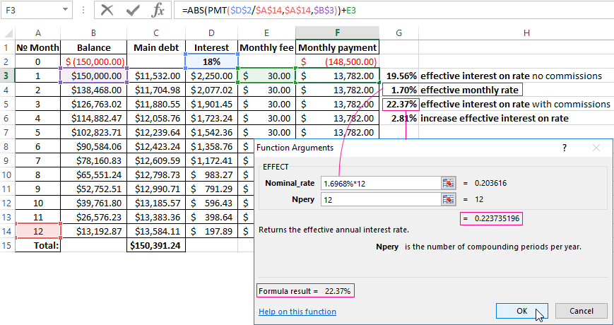
The monthly fees increased till 22, 37%. But in the loan contract will continue to be the figure of 18%. However, the new law requires banks to specify in the loan agreement to the effective annual interest rate. However, the borrower will see this figure after the approval and signing of the contract.
What distinguishes a lease from a loan
Leasing – this is the long-term rental of vehicles, real estate, equipment, with the possibility of their future redemption. The lessor acquires to the property and transfers it under the contract to a physical / legal person under certain conditions. The lessee uses to the property (in personal/ business purposes) and pays to the lessor for the right of using.
In the essen, it`s the same loan, only to the property will belong to the lessor until the lessee is fully repaid to the asset purchased plus interest.
The computation of the effective percent on leasing in Excel is followed on the same scheme as the computation of the annual interest rate on the credit. There is the example with another function.
The data input:
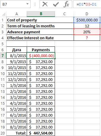
You can go on already blazed way: to computation the internal rate of return, and then multiply the result by 12. But we using the function =XIRR(it returns to the internal percent of return for the schedule of cash flows).
The function arguments:
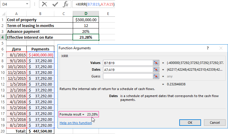
The effective interest on the lease was % to 23. 28%.
Calculation of the effective interest rate on OVDP in Excel
OVDP — domestic government loan bonds. They can be compared with the deposits in a bank. So how exactly the investor gets to a refund of the full amount of invested funds plus additional income as a percentage. The guarantor of the safety of funds is the National Bank.
The effective interest allows estimate to the real income, because it takes into account to capitalization of interest. For example, «acquire» one-year bonds in the sum of 50 000 at 17%. To calculate your income, using the function =FV():
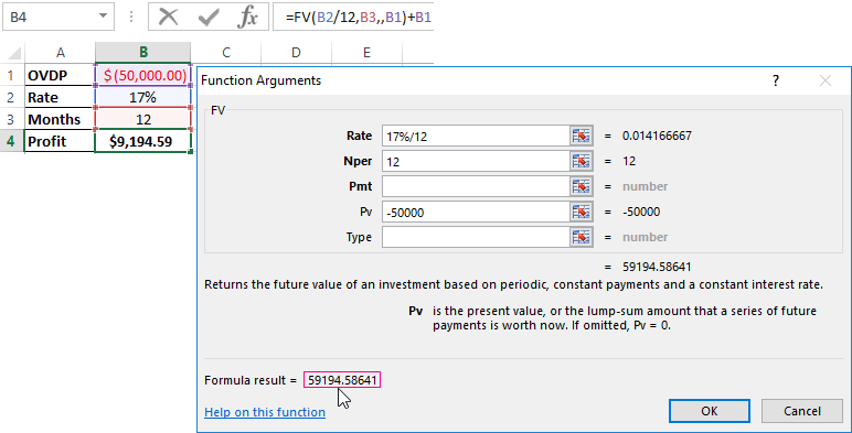
Suppose that the interest to capitalize by monthly. Therefore, we divide 17% by 12. The result as a decimal insertion we put in the field «Bet». In the «Nper» we enter to the number of periods of compounding. Monthly fixed payments we will not get, so the field «Pmt» leaving free. In the column «Pv» we put the deposit invested funds with the sign «-».
Download calculation effective interest rates in Excel
In the window, we immediately see to the sum, which you can get for the bonds in the end of the term. This is the monetary value of accrued compound interest.
Financial choices play a critical role in the development and execution of corporate strategies and plans. In daily life, we also face a slew of financial choices. For instance, suppose you’re applying for a loan to purchase a new automobile. It will undoubtedly be beneficial to discover the actual interest rate you will be required to pay your bank. Excel has the excel RATE function for such circumstances, which is specifically intended to calculate the interest rate for a certain term.
Table of Contents
- Excel rate function
- RATE formula Examples
- Determine a Loan’s Monthly Interest Rate
- Related Functions
Excel rate function
RATE is an Excel financial function that calculates the interest rate on an annuity over a specified time. The function calculates iteratively and may return zero or more solutions.
Excel 365, Excel 2019, Excel 2016, Excel 2013, Excel 2010, and Excel 2007 all provide this feature.
The following is the syntax:
=RATE(nper, pmt, pv, [fv], [type], [guess])
Where:
Nper(needed) – the total number of payment periods, which may include years, months, and quarters.Pmt(mandatory) – the set monthly payment amount that cannot be adjusted throughout the annuity’s life. It typically includes principle and interest but excludes taxes.Pv(needed) – the present value of the loan or investment, i.e. its current worth.Fv(optional) – the future value, that is, the cash balance you desire to have after the previous payment. If omitted, the default value is 0.Type(optional) – specifies the manner in which payments are made:0 or omitted(default) – payment is due at the end of the termGuess(optional) – your best guess for the rate. If left blank, it defaults to 10%.
Note:
- The RATE function performs trial and error calculations. If it does not reach a solution after 20 iterations, it returns a
#NUM!error. - By default, interest is computed on a per-payment basis. However, as seen in this example, you can get an annuity solve for interest rate by multiplying.
- While the RATE syntax specifies pv as a mandatory parameter, it may actually be removed if the fv argument is included. Typically, this syntax is used to calculate the interest rate on a savings account.
- In most circumstances, the guess parameter may be deleted since it serves just as a beginning value for an iterative method.
- When computing RATE for various periods, ensure that the values for nper and guess are constant. For instance, if you’re making yearly payments on a two-year loan with an annual interest rate of 4%, use 2 for nper and 4% for estimate.
- If you’re making monthly payments on the same loan, use 2*12 for the nper and 4% /12 for the estimate.
RATE formula Examples
In this example, we’ll look at the easiest way to create a RATE formula in Excel for the purpose of calculating interest rates.
Assume you borrowed $20,000 and are required to repay it in full over the following three years. You intend to pay three annual payments of $7200 each. How much will interest cost on a yearly basis?
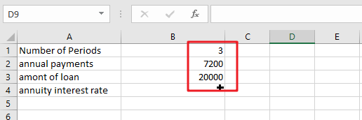
Please note that the yearly payment (pmt) is specified as a negative figure since it is an outgoing cash payment.
Assuming that the payment will be paid at the end of each year, we may omit or change the parameter to the default value. Also deleted are the two optional parameters and guess.
As a consequence, we get the following straightforward formula:
=RATE(B1,B2,B3)
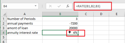
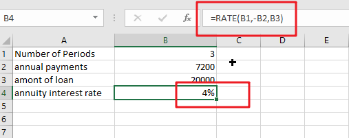
If the payment must be recorded as a positive integer, include the negative sign exactly before the pmt parameter in the formula:
=RATE(B1,-B2,B3)
Now that you’re familiar with the fundamentals of utilizing RATE in Excel, let’s look at a few particular use scenarios.
Determine a Loan’s Monthly Interest Rate
Given that the majority of installment loans are repaid monthly, it may be advantageous to know the monthly interest rate, correct? This is accomplished by providing an adequate number of payment periods to the RATE function.
Assume the loan is to be repaid in monthly installments over a two-year period. We multiply two years by twelve months to get the total amount of payments (2*12=24).
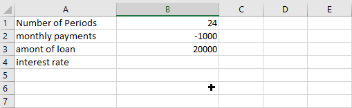
The remaining parameters are listed below:
- Nper (number of periods) in A1: 24
- Pmt (monthly payment) in A2: -1000
- Pv(load amount) in A3: 20000
Assuming the payment is due at the end of each month, the monthly interest rate may be calculated using the well-known formula:
=RATE(B1,B2,B3)
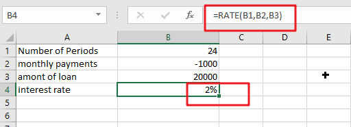
Calculate the interest rate on a monthly basis in Excel
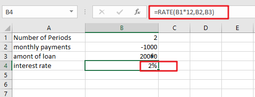
If your source data contains the number of years required to repay the loan, you may do the multiplication inside the nper argument:
=RATE(B1*12,B2,B3)
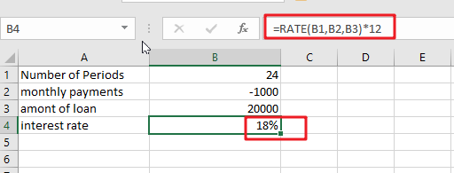
Calculate annuity for Interest rate on Monthly Payments
Continuing our example, how do you calculate the yearly interest rate on monthly payments? Simply multiply the RATE value by the number of periods in a year, which in our instance is twelve:
=RATE(B1,B2,B3)*12
Calculate Quarterly Interest Rate
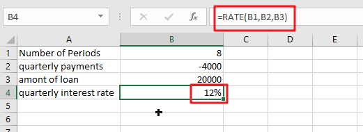
Assume the loan is to be repaid in quarterly installments over a two-year period. We multiply two years by 4 quarters to get the total amount of payments (2*4=8).
To begin, the entire number of periods is converted to quarterly:
Nper: 2 (years) multiplied by 4 (quarters per year) equals 8.
Then, compute the quarterly interest rate in cell B4 using the RATE function:
=RATE(B1,B2,B3)
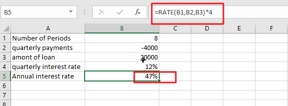
If you want to get the yearly interest rate based on quarterly interest rate, you still need to multiply the quarterly interest rate by four, using the following formula:
=RATE(B1,B2,B3)*4
- Excel RATE function
The Excel RATE function returns the interest rate per payment period of an annuity.The syntax of the RATE function is as below:=RATE(nper, pmt,pv,[fv],[type],[guess])….
Содержание
- RATE function
- Description
- Syntax
- Remarks
- Example
- How to calculate compound interest for an intra-year period in Excel
- Summary
- Calculating Future Value of Intra-Year Compound Interest
- Examples
- Using Excel formulas to figure out payments and savings
- Calculation of the effective interest rate on loan in Excel
- The calculation of the effective rate on the loan in Excel
- What distinguishes a lease from a loan
- Calculation of the effective interest rate on OVDP in Excel
RATE function
This article describes the formula syntax and usage of the RATE function in Microsoft Excel.
Description
Returns the interest rate per period of an annuity. RATE is calculated by iteration and can have zero or more solutions. If the successive results of RATE do not converge to within 0.0000001 after 20 iterations, RATE returns the #NUM! error value.
Syntax
RATE(nper, pmt, pv, [fv], [type], [guess])
Note: For a complete description of the arguments nper, pmt, pv, fv, and type, see PV.
The RATE function syntax has the following arguments:
Nper Required. The total number of payment periods in an annuity.
Pmt Required. The payment made each period and cannot change over the life of the annuity. Typically, pmt includes principal and interest but no other fees or taxes. If pmt is omitted, you must include the fv argument.
Pv Required. The present value — the total amount that a series of future payments is worth now.
Fv Optional. The future value, or a cash balance you want to attain after the last payment is made. If fv is omitted, it is assumed to be 0 (the future value of a loan, for example, is 0). If fv is omitted, you must include the pmt argument.
Type Optional. The number 0 or 1 and indicates when payments are due.
Set type equal to
If payments are due
At the end of the period
At the beginning of the period
Guess Optional. Your guess for what the rate will be.
If you omit guess, it is assumed to be 10 percent.
If RATE does not converge, try different values for guess. RATE usually converges if guess is between 0 and 1.
Make sure that you are consistent about the units you use for specifying guess and nper. If you make monthly payments on a four-year loan at 12 percent annual interest, use 12%/12 for guess and 4*12 for nper. If you make annual payments on the same loan, use 12% for guess and 4 for nper.
Example
Copy the example data in the following table, and paste it in cell A1 of a new Excel worksheet. For formulas to show results, select them, press F2, and then press Enter. If you need to, you can adjust the column widths to see all the data.
Источник
How to calculate compound interest for an intra-year period in Excel
Summary
The future value of a dollar amount, commonly called the compounded value, involves the application of compound interest to a present value amount. The result is a future dollar amount. Three types of compounding are
annual, intra-year, and annuity compounding. This article discusses intra-year calculations for compound interest.
For additional information about annual compounding, view the following article:
Calculating Future Value of Intra-Year Compound Interest
Intra-year compound interest is interest that is compounded more frequently than once a year. Financial institutions may calculate interest on bases of semiannual, quarterly, monthly, weekly, or even daily time periods.
Microsoft Excel includes the EFFECT function in the Analysis ToolPak add-in for versions older than 2003. The Analysis ToolPak is already loaded. The EFFECT function returns the compounded interest rate based on the annual interest rate and the number of compounding periods per year.
The formula to calculate intra-year compound interest with the EFFECT worksheet function is as follows:
The general equation to calculate compound interest is as follows
where the following is true:
P = initial principal
k = annual interest rate paid
m = number of times per period (typically months) the interest is compounded
n = number of periods (typically years) or term of the loan
Examples
The examples in this section use the EFFECT function, the general equation, and the following sample data:
Источник
Using Excel formulas to figure out payments and savings
Managing personal finances can be a challenge, especially when trying to plan your payments and savings. Excel formulas and budgeting templates can help you calculate the future value of your debts and investments, making it easier to figure out how long it will take for you to reach your goals. Use the following functions:
PMT calculates the payment for a loan based on constant payments and a constant interest rate.
NPER calculates the number of payment periods for an investment based on regular, constant payments and a constant interest rate.
PV returns the present value of an investment. The present value is the total amount that a series of future payments is worth now.
FV returns the future value of an investment based on periodic, constant payments and a constant interest rate.
Figure out the monthly payments to pay off a credit card debt
Assume that the balance due is $5,400 at a 17% annual interest rate. Nothing else will be purchased on the card while the debt is being paid off.
Using the function PMT(rate,NPER,PV)
the result is a monthly payment of $266.99 to pay the debt off in two years.
The rate argument is the interest rate per period for the loan. For example, in this formula the 17% annual interest rate is divided by 12, the number of months in a year.
The NPER argument of 2*12 is the total number of payment periods for the loan.
The PV or present value argument is 5400.
Figure out monthly mortgage payments
Imagine a $180,000 home at 5% interest, with a 30-year mortgage.
Using the function PMT(rate,NPER,PV)
the result is a monthly payment (not including insurance and taxes) of $966.28.
The rate argument is 5% divided by the 12 months in a year.
The NPER argument is 30*12 for a 30 year mortgage with 12 monthly payments made each year.
The PV argument is 180000 (the present value of the loan).
Find out how to save each month for a dream vacation
You’d like to save for a vacation three years from now that will cost $8,500. The annual interest rate for saving is 1.5%.
Using the function PMT(rate,NPER,PV,FV)
to save $8,500 in three years would require a savings of $230.99 each month for three years.
The rate argument is 1.5% divided by 12, the number of months in a year.
The NPER argument is 3*12 for twelve monthly payments over three years.
The PV (present value) is 0 because the account is starting from zero.
The FV (future value) that you want to save is $8,500.
Now imagine that you are saving for an $8,500 vacation over three years, and wonder how much you would need to deposit in your account to keep monthly savings at $175.00 per month. The PV function will calculate how much of a starting deposit will yield a future value.
Using the function PV(rate,NPER,PMT,FV)
an initial deposit of $1,969.62 would be required in order to be able to pay $175.00 per month and end up with $8500 in three years.
The rate argument is 1.5%/12.
The NPER argument is 3*12 (or twelve monthly payments for three years).
The PMT is -175 (you would pay $175 per month).
The FV (future value) is 8500.
Find out how long it will take to pay off a personal loan
Imagine that you have a $2,500 personal loan, and have agreed to pay $150 a month at 3% annual interest.
Using the function NPER(rate,PMT,PV)
it would take 17 months and some days to pay off the loan.
The rate argument is 3%/12 monthly payments per year.
The PMT argument is -150.
The PV (present value) argument is 2500.
Figure out a down payment
Say that you’d like to buy a $19,000 car at a 2.9% interest rate over three years. You want to keep the monthly payments at $350 a month, so you need to figure out your down payment. In this formula the result of the PV function is the loan amount, which is then subtracted from the purchase price to get the down payment.
Using the function PV(rate,NPER,PMT)
the down payment required would be $6,946.48
The $19,000 purchase price is listed first in the formula. The result of the PV function will be subtracted from the purchase price.
The rate argument is 2.9% divided by 12.
The NPER argument is 3*12 (or twelve monthly payments over three years).
The PMT is -350 (you would pay $350 per month).
See how much your savings will add up to over time
Starting with $500 in your account, how much will you have in 10 months if you deposit $200 a month at 1.5% interest?
Using the function FV(rate,NPER,PMT,PV)
in 10 months you would have $2,517.57 in savings.
Источник
Calculation of the effective interest rate on loan in Excel
The effective rate of interest on the loan (as with almost on any other financial instrument) – this is the expression of all future cash payments (incomes from a financial instrument), which are included in the treaty provision of the contract, in the figure annual interest. That is the real interest that the debtor will pay for using of money in the Bank (investor – to obtain). Here is taken into account the rate of interest designated in the contract, all fees, repayment schemes, loan term (of deposit).
The calculation of the effective rate on the loan in Excel
There are the range of built-in functions in Excel, that allow you to compute the effective rate of interest, with taking into account additional charges and fees, and excluding (relying only on the nominal interest and the loan term).
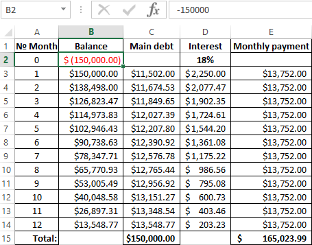
The debtor took a credit in the sum of 150 000$ on the term of 1 year (12 months). The nominal annual rate — is 18%. Payments on the loan specify in the table below:
Since this example does not include the additional fees and charges, we determine to the annual effective rate using the function EFFECT.
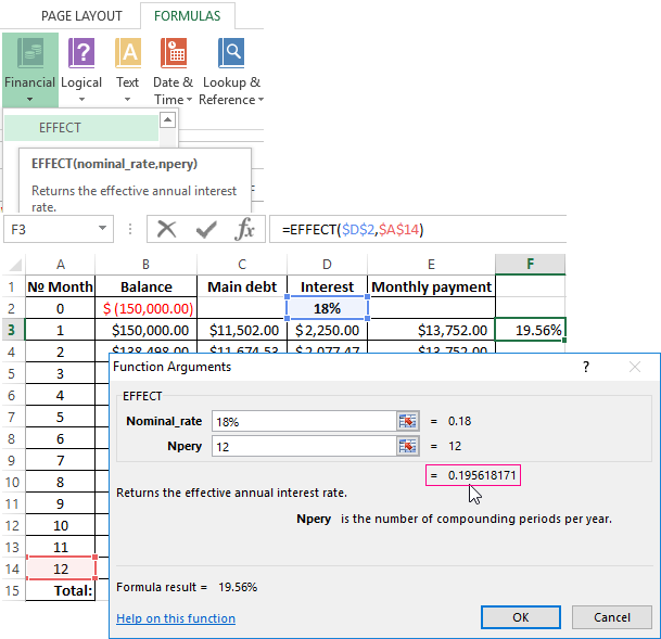
We are calling: «FORMULAS»-«Function Library»-«Financial» finding the function EFFECT. The arguments:
- «Nominal rate» — is the annual rate of interest on the credit, which is designated in the agreement with the Bank. In this example – is 18% (0, 18).
- «Number of periods» — the number of periods in a year, for which interests are charged. In this example – there are 12 months.
The effective interest on rate — is 19. 56%.
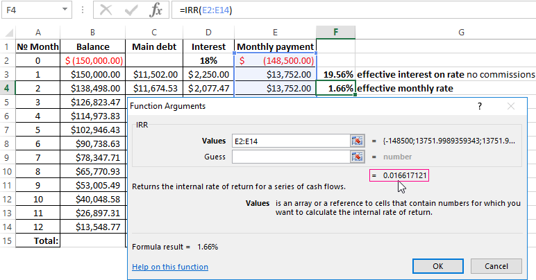
Let’s complicate the task by adding the one-time commission loan at the amount of 1% of the sum of 150 000$. In monetary terms – is 1500$. So, the borrower to get on his hands is the sum of 148 500$.
For calculating to the effective monthly rate, we need use the IRR function (return to the internal rate of return for cash flow):
We have made the column with monthly payments 148 500 with the sign «-», because the money the Bank first gives. Payments which the debtor will make in the cashier subsequently are positive for the bank. The internal rate of return we consider from the Bank’s point of view: it acts as an investor.
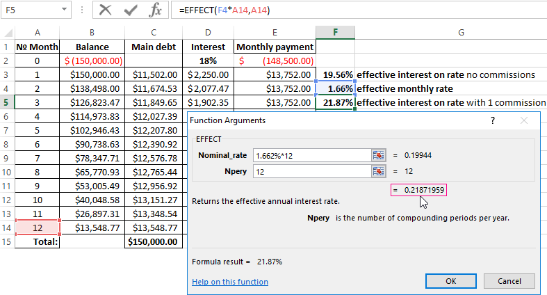
The function has given to the effective monthly rate of 1.6617121%. For the calculating of the nominal rate to the result need multiply by 12 (the term of loan): 1.662% * 12 = 19.94%. Let`s recalculate the effective interest percent:
The one-time fee in amount of 1% increased the actual annual interest on 2.31%. It was: 21, 87%.
We add in the scheme of payments on the loan to the monthly fee for account maintenance in the amount of 30$. Monthly effective rate will be equal to 1.6968%.
The nominal percent is 1.6968% * 12 = is 20.3616%. The effective annual rate is:
The monthly fees increased till 22, 37%. But in the loan contract will continue to be the figure of 18%. However, the new law requires banks to specify in the loan agreement to the effective annual interest rate. However, the borrower will see this figure after the approval and signing of the contract.
What distinguishes a lease from a loan
Leasing – this is the long-term rental of vehicles, real estate, equipment, with the possibility of their future redemption. The lessor acquires to the property and transfers it under the contract to a physical / legal person under certain conditions. The lessee uses to the property (in personal/ business purposes) and pays to the lessor for the right of using.
In the essen, it`s the same loan, only to the property will belong to the lessor until the lessee is fully repaid to the asset purchased plus interest.
The computation of the effective percent on leasing in Excel is followed on the same scheme as the computation of the annual interest rate on the credit. There is the example with another function.
You can go on already blazed way: to computation the internal rate of return, and then multiply the result by 12. But we using the function =XIRR(it returns to the internal percent of return for the schedule of cash flows).
The function arguments:
The effective interest on the lease was % to 23. 28%.
Calculation of the effective interest rate on OVDP in Excel
OVDP — domestic government loan bonds. They can be compared with the deposits in a bank. So how exactly the investor gets to a refund of the full amount of invested funds plus additional income as a percentage. The guarantor of the safety of funds is the National Bank.
The effective interest allows estimate to the real income, because it takes into account to capitalization of interest. For example, «acquire» one-year bonds in the sum of 50 000 at 17%. To calculate your income, using the function =FV():
Suppose that the interest to capitalize by monthly. Therefore, we divide 17% by 12. The result as a decimal insertion we put in the field «Bet». In the «Nper» we enter to the number of periods of compounding. Monthly fixed payments we will not get, so the field «Pmt» leaving free. In the column «Pv» we put the deposit invested funds with the sign «-».
In the window, we immediately see to the sum, which you can get for the bonds in the end of the term. This is the monetary value of accrued compound interest.
Источник
Purpose
Get the interest rate per period of an annuity
Return value
The interest rate per period
Usage notes
The RATE function returns the interest rate per period of an annuity. You can use RATE to calculate the periodic interest rate, then multiply as required to derive the annual interest rate. The RATE function calculates by iteration. If the results of RATE do not converge within 20 iterations, RATE returns the #NUM! error value.
The RATE function takes six separate arguments, three of which are required as explained below.
nper (required) — The total number of payment periods in the annuity. For example, a 5-year car loan with monthly payments has 60 periods. You can enter nper as 5*12 to show how the number was determined.
pmt (required) — The payment made each period. This number cannot change over the life of the annuity. In annuity functions, cash paid out is represented by a negative number. Note: If pmt is not provided, the optional fv argument must be supplied.
pv (optional) — The present value. This is the cash balance required after all payments have been made.
fv (optional) — The future value, or a cash balance required after the last payment is made. When fv is omitted, it defaults to zero (0) and pmt must be provided.
type (optional) — type is a boolean that controls when when payments are due. Use 0 for payments due at the end of the period (regular annuities) and 1 for payments due at the end of the period (annuities due). Type defaults to 0 (end of period).
guess (optional) — guess is a seed value to use for iteration. When omitted, guess defaults to 10%. Ordinarily, you can safely omit guess. If RATE does not converge, RATE will return a #NUM! error. Try different values for guess between 0 and 1.
Example
To calculate the annual interest rate for a $5000 loan with payments of $93.22 per month over 5 years, you can use RATE in a formula like this:
=RATE(60,-93.22,5000)*12 // returns 4.5%
In the example shown, the formula in C10 is:
=RATE(C7,-C6,C5)*C8 // returns 4.5%
Notice the value for pmt from C6 is entered as a negative value.
Notes
You must use consistent values for for guess and nper. If you make monthly payments on a five-year loan at 10 percent annual interest, use 10%/12 for guess and 5*12 for nper. If you make annual payments on the same loan, use 10% for guess and 5 for nper.