Interest rate functions excel

This article describes the formula syntax and usage of the RATE function in Microsoft Excel.

Description

Returns the interest rate per period of an annuity. RATE is calculated by iteration and can have zero or more solutions. If the successive results of RATE do not converge to within 0.0000001 after 20 iterations, RATE returns the #NUM! error value.

Syntax

RATE(nper, pmt, pv, [fv], [type], [guess])

Note: For a complete description of the arguments nper, pmt, pv, fv, and type, see PV.

The RATE function syntax has the following arguments:

• Nper    Required. The total number of payment periods in an annuity.

• Pmt    Required. The payment made each period and cannot change over the life of the annuity. Typically, pmt includes principal and interest but no other fees or taxes. If pmt is omitted, you must include the fv argument.

• Pv    Required. The present value — the total amount that a series of future payments is worth now.

• Fv    Optional. The future value, or a cash balance you want to attain after the last payment is made. If fv is omitted, it is assumed to be 0 (the future value of a loan, for example, is 0). If fv is omitted, you must include the pmt argument.

• Type    Optional. The number 0 or 1 and indicates when payments are due.

Set type equal to	If payments are due
0 or omitted	At the end of the period
1	At the beginning of the period

• Guess    Optional. Your guess for what the rate will be.

  • If you omit guess, it is assumed to be 10 percent.

  • If RATE does not converge, try different values for guess. RATE usually converges if guess is between 0 and 1.

Remarks

Make sure that you are consistent about the units you use for specifying guess and nper. If you make monthly payments on a four-year loan at 12 percent annual interest, use 12%/12 for guess and 4*12 for nper. If you make annual payments on the same loan, use 12% for guess and 4 for nper.

Example

Copy the example data in the following table, and paste it in cell A1 of a new Excel worksheet. For formulas to show results, select them, press F2, and then press Enter. If you need to, you can adjust the column widths to see all the data.

Data	Description
4	Years of the loan
-200	Monthly payment
8000	Amount of the loan
Formula	Description	Result
=RATE(A2*12, A3, A4)	Monthly rate of the loan with the terms entered as arguments in A2:A4.	1%
=RATE(A2*12, A3, A4)*12	Annual rate of the loan with the same terms.	9.24%

Date yes Add (Subtract) Days to a Date Concatenate Dates Convert Date to Number Convert Date to Text Month Name to Number Create Date Range from Dates Day Number of Year Month Name from Date First Day of Month Add (Subtract) Weeks to a Date If Functions with Dates Max Date Number of Days Between Dates Number of Days in a Month Number of Weeks Between Dates Number of Years Between Dates Split Date & Time into Separate Cells Countdown Remaining Days Insert Dates Random Date Generator Using Dynamic Ranges — Year to Date Values Add (Subtract) Years to a Date Date Formula Examples Extract Day from Date Get Day Name from Date Count Days Left in Month / Year Count Workdays Left in Month / Year Get Last Day of Month Last Business Day of Month / Year Number of Work / Business Days in Month Weekday Abbreviations Auto Populate Dates Number of Months Between Dates Quarter from a Date Years of Service Change Date Format Compare Dates Time yes Add (Subtract) Hours to Time Add (Subtract) Minutes to Time Add (Subtract) Seconds to Time Add Up time (Total Time) Time Differences Change Time Format Convert Minutes to Hours Convert Time to Decimal Convert Time to Hours Convert Time to Minutes Convert Time to Seconds Military Time Round Time to Nearest 15 Minutes Overtime Calculator Number of Hours Between Times Convert Seconds to Minutes, Hours, or Time Count Hours Worked Time Differences Time Format — Show Minutes Seconds Text yes Add Commas to Cells Get First Word from Text Capitalize First Letter Clean & Format Phone #s Remove Extra Trailing / Leading Spaces Add Spaces to Cell Assign Number Value to Text Combine Cells with Comma Combine First and Last Names Convert Text String to Date Convert Text to Number Extract Text From Cell Get Last Word Remove Unwated Characters Extract Text Before or After Character How to Split Text String by Space, Comma, & More Remove Special Characters Remove First Characters from Left Substitute Multiple Values Switch First & Last Names w/ Commas Remove Specific Text from a Cell Extract Text Between Characters (Ex. Parenthesis) Add Leading Zeros to a Number Remove Line Breaks from Text Remove all Numbers from Text Reverse Text Remove Non-Numeric Characters Remove Last Character(s) From Right Separate First and Last Names Separate Text & Numbers Round yes Round Formulas Round Price to Nearest Dollar or Cent Round to Nearest 10, 100, or 1000 Round to Nearest 5 or .5 Round Percentages Round to Significant Figures Count yes Count Blank and Non-blank Cells Count Cells Between Two Numbers Count Cells not Equal to Count if Cells are in Range Count Times Word Appears in Cell Count Words in Cell Count Specific Characters in Column Count Total Number of Characters in Column Count Cells that Equal one of two Results Count Cells that do not Contain Count Cells that Contain Specific Text Count Unique Values in Range Countif — Multiple Criteria Count Total Number of Cells in Range Count Cells with Any Text Count Total Cells in a Table Lookup yes Two Dimensional VLOOKUP VLOOKUP Simple Example Vlookup — Multiple Matches Case Sensitive Lookup Case Sensitive VLOOKUP Sum if — VLOOKUP Case Sensitive Lookup Case Sensitive VLOOKUP Find Duplicates w/ VLOOKUP or MATCH INDEX MATCH MATCH Lookup — Return Cell Address (Not Value) Lookup Last Value in Column or Row Reverse VLOOKUP (Right to Left) Risk Score Bucket with VLOOKUP Sum with a VLOOKUP Function VLOOKUP & INDIRECT VLOOKUP Concatenate VLOOKUP Contains (Partial Match) 17 Reasons Why Your XLOOKUP is Not Working Double (Nested) XLOOKUP — Dynamic Columns IFERROR (& IFNA) XLOOKUP Lookup Min / Max Value Nested VLOOKUP Top 11 Alternatives to VLOOKUP (Updated 2022!) VLOOKUP – Dynamic Column Reference VLOOKUP – Fix #N/A Error VLOOKUP – Multiple Sheets at Once VLOOKUP & HLOOKUP Combined VLOOKUP & MATCH Combined VLOOKUP Between Worksheets or Spreadsheets VLOOKUP Duplicate Values VLOOKUP Letter Grades VLOOKUP Return Multiple Columns VLOOKUP Returns 0? Return Blank Instead VLOOKUP w/o #N/A Error XLOOKUP Multiple Sheets at Once XLOOKUP Between Worksheets or Spreadsheets XLOOKUP by Date XLOOKUP Duplicate Values XLOOKUP Multiple Criteria XLOOKUP Return Multiple Columns XLOOKUP Returns 0? Return Blank Instead XLOOKUP Text XLOOKUP with IF XLOOKUP With If Statement Misc. yes Sort Multiple Columns Use Cell Value in Formula Percentage Change Between Numbers Percentage Breakdown Rank Values Add Spaces to Cell CAGR Formula Average Time Decimal Part of Number Integer Part of a Number Compare Items in a List Dealing with NA() Errors Get Worksheet Name Wildcard Characters Hyperlink to Current Folder Compound Interest Formula Percentage Increase Create Random Groups Sort with the Small and Large Functions Non-volatile Function Alternatives Decrease a Number by a Percentage Calculate Percent Variance Profit Margin Calculator Convert Column Number to Letter Get Full Address of Named Range Insert File Name Insert Path Latitute / Longitude Functions Replace Negative Values Reverse List Range Convert State Name to Abbreviation Create Dynamic Hyperlinks Custom Sort List with Formula Data Validation — Custom Formulas Dynamic Sheet Reference (INDIRECT) Reference Cell in Another Sheet or Workbook Get Cell Value by Address Get Worksheet Name Increment Cell Reference List Sheet Names List Skipped Numbers in Sequence Return Address of Max Value in Range Search by Keywords Select Every Other (or Every nth) Row Basics yes Cell Reference Basics — A1, R1C1, 3d, etc. Add Up (Sum) Entire Column or Row Into to Dynamic Array Formulas Conversions yes Convert Time Zones Convert Celsius to Fahrenheit Convert Pounds to Kilograms Convert Time to Unix Time Convert Feet to Meters Convert Centimeters to Inches Convert Kilometers to Miles Convert Inches to Feet Convert Date to Julian Format Convert Column Letter to Number Tests yes Test if a Range Contains any Text Test if any Cell in Range is Number Test if a Cell Contains a Specific Value Test if Cell Contains Any Number Test if Cell Contains Specific Number Test if Cell is Number or Text If yes Percentile If Subtotal If Sumproduct If Large If and Small If Median If Concatentate If Max If Rank If TEXTJOIN If Sum yes Sum if — Begins With / Ends With Sum if — Month or Year to Date Sum if — By Year Sum if — Blank / Non-Blank Sum if — Horizontal Sum Count / Sum If — Cell Color INDIRECT Sum Sum If — Across Multiple Sheets Sum If — By Month Sum If — Cells Not Equal To Sum If — Not Blank Sum if — Between Values Sum If — Week Number Sum Text Sum if — By Category or Group Sum if — Cell Contains Specific Text (Wildcards) Sum if — Date Rnage Sum if — Dates Equal Sum if — Day of Week Sum if — Greater Than Sum if — Less Than Average yes Average Non-Zero Values Average If — Not Blank Average — Ignore 0 Average — Ignore Errors Math yes Multiplication Table Cube Roots nth Roots Square Numbers Square Roots Calculations yes Calculate a Ratio Calculate Age KILLLLLLL Calculate Loan Payments GPA Formula Calculate VAT Tax How to Grade Formulas Find yes Find a Number in a Column / Workbook Find Most Frequent Numbers Find Smallest n Values Find nth Occurance of Character in Text Find and Extract Number from String Find Earliest or Latest Date Based on Criteria Find First Cell with Any Value Find Last Row Find Last Row with Data Find Missing Values Find Largest n Values Most Frequent Number Conditional Formatting yes Conditional Format — Dates & Times Conditional Format — Highlight Blank Cells New Functions XLOOKUP Replaces VLOOKUP, HLOOKUP, and INDEX / MATCH Logical yes AND Checks whether all conditions are met. TRUE/FALSE IF If condition is met, do something, if not, do something else. IFERROR If result is an error then do something else. NOT Changes TRUE to FALSE and FALSE to TRUE. OR Checks whether any conditions are met. TRUE/FALSE XOR Checks whether one and only one condition is met. TRUE/FALSE Lookup & Reference yes FALSE The logical value: FALSE. TRUE The logical value: TRUE. ADDRESS Returns a cell address as text. AREAS Returns the number of areas in a reference. CHOOSE Chooses a value from a list based on it’s position number. COLUMN Returns the column number of a cell reference. COLUMNS Returns the number of columns in an array. HLOOKUP Lookup a value in the first row and return a value. HYPERLINK Creates a clickable link. INDEX Returns a value based on it’s column and row numbers. INDIRECT Creates a cell reference from text. LOOKUP Looks up values either horizontally or vertically. MATCH Searches for a value in a list and returns its position. OFFSET Creates a reference offset from a starting point. ROW Returns the row number of a cell reference. ROWS Returns the number of rows in an array. TRANSPOSE Flips the oriention of a range of cells. VLOOKUP Lookup a value in the first column and return a value. Date & Time yes DATE Returns a date from year, month, and day. DATEDIF Number of days, months or years between two dates. DATEVALUE Converts a date stored as text into a valid date DAY Returns the day as a number (1-31). DAYS Returns the number of days between two dates. DAYS360 Returns days between 2 dates in a 360 day year. EDATE Returns a date, n months away from a start date. EOMONTH Returns the last day of the month, n months away date. HOUR Returns the hour as a number (0-23). MINUTE Returns the minute as a number (0-59). MONTH Returns the month as a number (1-12). NETWORKDAYS Number of working days between 2 dates. NETWORKDAYS.INTL Working days between 2 dates, custom weekends. NOW Returns the current date and time. SECOND Returns the second as a number (0-59) TIME Returns the time from a hour, minute, and second. TIMEVALUE Converts a time stored as text into a valid time. TODAY Returns the current date. WEEKDAY Returns the day of the week as a number (1-7). WEEKNUM Returns the week number in a year (1-52). WORKDAY The date n working days from a date. WORKDAY.INTL The date n working days from a date, custom weekends. YEAR Returns the year. YEARFRAC Returns the fraction of a year between 2 dates. Engineering yes CONVERT Convert number from one unit to another. Financial yes FV Calculates the future value. PV Calculates the present value. NPER Calculates the total number of payment periods. PMT Calculates the payment amount. RATE Calculates the interest Rate. NPV Calculates the net present value. IRR The internal rate of return for a set of periodic CFs. XIRR The internal rate of return for a set of non-periodic CFs. PRICE Calculates the price of a bond. YIELD Calculates the bond yield. INTRATE The interest rate of a fully invested security. Information yes CELL Returns information about a cell. ERROR.TYPE Returns a value representing the cell error. ISBLANK Test if cell is blank. TRUE/FALSE ISERR Test if cell value is an error, ignores #N/A. TRUE/FALSE ISERROR Test if cell value is an error. TRUE/FALSE ISEVEN Test if cell value is even. TRUE/FALSE ISFORMULA Test if cell is a formula. TRUE/FALSE ISLOGICAL Test if cell is logical (TRUE or FALSE). TRUE/FALSE ISNA Test if cell value is #N/A. TRUE/FALSE ISNONTEXT Test if cell is not text (blank cells are not text). TRUE/FALSE ISNUMBER Test if cell is a number. TRUE/FALSE ISODD Test if cell value is odd. TRUE/FALSE ISREF Test if cell value is a reference. TRUE/FALSE ISTEXT Test if cell is text. TRUE/FALSE N Converts a value to a number. NA Returns the error: #N/A. TYPE Returns the type of value in a cell. Math yes ABS Calculates the absolute value of a number. AGGREGATE Define and perform calculations for a database or a list. CEILING Rounds a number up, to the nearest specified multiple. COS Returns the cosine of an angle. DEGREES Converts radians to degrees. DSUM Sums database records that meet certain criteria. EVEN Rounds to the nearest even integer. EXP Calculates the exponential value for a given number. FACT Returns the factorial. FLOOR Rounds a number down, to the nearest specified multiple. GCD Returns the greatest common divisor. INT Rounds a number down to the nearest integer. LCM Returns the least common multiple. LN Returns the natural logarithm of a number. LOG Returns the logarithm of a number to a specified base. LOG10 Returns the base-10 logarithm of a number. MOD Returns the remainder after dividing. MROUND Rounds a number to a specified multiple. ODD Rounds to the nearest odd integer. PI The value of PI. POWER Calculates a number raised to a power. PRODUCT Multiplies an array of numbers. QUOTIENT Returns the integer result of division. RADIANS Converts an angle into radians. RAND Calculates a random number between 0 and 1. RANDBETWEEN Calculates a random number between two numbers. ROUND Rounds a number to a specified number of digits. ROUNDDOWN Rounds a number down (towards zero). ROUNDUP Rounds a number up (away from zero). SIGN Returns the sign of a number. SIN Returns the sine of an angle. SQRT Calculates the square root of a number. SUBTOTAL Returns a summary statistic for a series of data. SUM Adds numbers together. SUMIF Sums numbers that meet a criteria. SUMIFS Sums numbers that meet multiple criteria. SUMPRODUCT Multiplies arrays of numbers and sums the resultant array. TAN Returns the tangent of an angle. TRUNC Truncates a number to a specific number of digits. Stats yes AVERAGE Averages numbers. AVERAGEA Averages numbers. Includes text & FALSE =0, TRUE =1. AVERAGEIF Averages numbers that meet a criteria. AVERAGEIFS Averages numbers that meet multiple criteria. CORREL Calculates the correlation of two series. COUNT Counts cells that contain a number. COUNTA Count cells that are non-blank. COUNTBLANK Counts cells that are blank. COUNTIF Counts cells that meet a criteria. COUNTIFS Counts cells that meet multiple criteria. FORECAST Predict future y-values from linear trend line. FREQUENCY Counts values that fall within specified ranges. GROWTH Calculates Y values based on exponential growth. INTERCEPT Calculates the Y intercept for a best-fit line. LARGE Returns the kth largest value. LINEST Returns statistics about a trendline. MAX Returns the largest number. MEDIAN Returns the median number. MIN Returns the smallest number. MODE Returns the most common number. PERCENTILE Returns the kth percentile. PERCENTILE.INC Returns the kth percentile. Where k is inclusive. PERCENTILE.EXC Returns the kth percentile. Where k is exclusive. QUARTILE Returns the specified quartile value. QUARTILE.INC Returns the specified quartile value. Inclusive. QUARTILE.EXC Returns the specified quartile value. Exclusive. RANK Rank of a number within a series. RANK.AVG Rank of a number within a series. Averages. RANK.EQ Rank of a number within a series. Top Rank. SLOPE Calculates the slope from linear regression. SMALL Returns the kth smallest value. STDEV Calculates the standard deviation. STDEV.P Calculates the SD of an entire population. STDEV.S Calculates the SD of a sample. STDEVP Calculates the SD of an entire population TREND Calculates Y values based on a trendline. Text yes CHAR Returns a character specified by a code. CLEAN Removes all non-printable characters. CODE Returns the numeric code for a character. CONCATENATE Combines text together. DOLLAR Converts a number to text in currency format. EXACT Test if cells are exactly equal. Case-sensitive. TRUE/FALSE FIND Locates position of text within a cell.Case-sensitive. LEFT Truncates text a number of characters from the left. LEN Counts number of characters in text. LOWER Converts text to lower case. MID Extracts text from the middle of a cell. PROPER Converts text to proper case. REPLACE Replaces text based on it’s location. REPT Repeats text a number of times. RIGHT Truncates text a number of characters from the right. SEARCH Locates position of text within a cell.Not Case-sensitive. SUBSTITUTE Finds and replaces text. Case-sensitive. TEXT Converts a value into text with a specific number format. TRIM Removes all extra spaces from text. UPPER Converts text to upper case. VALUE Converts a number stored as text into a number.

Purpose 

Return value 

Usage notes 

The effective rate of interest on the loan (as with almost on any other financial instrument) – this is the expression of all future cash payments (incomes from a financial instrument), which are included in the treaty provision of the contract, in the figure annual interest. That is the real interest that the debtor will pay for using of money in the Bank (investor – to obtain). Here is taken into account the rate of interest designated in the contract, all fees, repayment schemes, loan term (of deposit).



The calculation of the effective rate on the loan in Excel

There are the range of built-in functions in Excel, that allow you to compute the effective rate of interest, with taking into account additional charges and fees, and excluding (relying only on the nominal interest and the loan term).

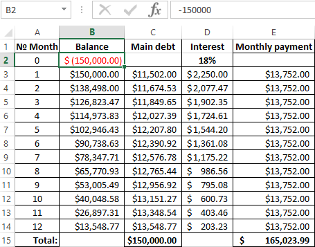
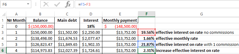
The debtor took a credit in the sum of 150 000$ on the term of 1 year (12 months). The nominal annual rate — is 18%. Payments on the loan specify in the table below:

Since this example does not include the additional fees and charges, we determine to the annual effective rate using the function EFFECT.

We are calling: «FORMULAS»-«Function Library»-«Financial» finding the function EFFECT. The arguments:

1. «Nominal rate» — is the annual rate of interest on the credit, which is designated in the agreement with the Bank. In this example – is 18% (0, 18).
2. «Number of periods» — the number of periods in a year, for which interests are charged. In this example – there are 12 months.

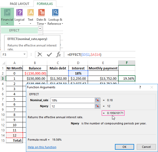
The effective interest on rate — is 19. 56%.

Let’s complicate the task by adding the one-time commission loan at the amount of 1% of the sum of 150 000$. In monetary terms – is 1500$. So, the borrower to get on his hands is the sum of 148 500$.

For calculating to the effective monthly rate, we need use the IRR function (return to the internal rate of return for cash flow):

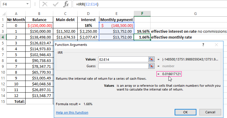
We have made the column with monthly payments 148 500 with the sign «-», because the money the Bank first gives. Payments which the debtor will make in the cashier subsequently are positive for the bank. The internal rate of return we consider from the Bank’s point of view: it acts as an investor.

The function has given to the effective monthly rate of 1.6617121%. For the calculating of the nominal rate to the result need multiply by 12 (the term of loan): 1.662% * 12 = 19.94%. Let`s recalculate the effective interest percent:

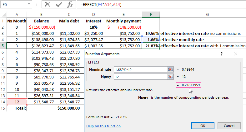
The one-time fee in amount of 1% increased the actual annual interest on 2.31%. It was: 21, 87%.

We add in the scheme of payments on the loan to the monthly fee for account maintenance in the amount of 30$. Monthly effective rate will be equal to 1.6968%.

The nominal percent is 1.6968% * 12 = is 20.3616%. The effective annual rate is:

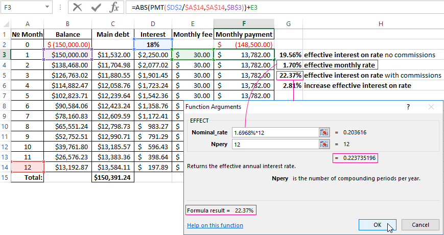
The monthly fees increased till 22, 37%. But in the loan contract will continue to be the figure of 18%. However, the new law requires banks to specify in the loan agreement to the effective annual interest rate. However, the borrower will see this figure after the approval and signing of the contract.



What distinguishes a lease from a loan

Leasing – this is the long-term rental of vehicles, real estate, equipment, with the possibility of their future redemption. The lessor acquires to the property and transfers it under the contract to a physical / legal person under certain conditions. The lessee uses to the property (in personal/ business purposes) and pays to the lessor for the right of using.

In the essen, it`s the same loan, only to the property will belong to the lessor until the lessee is fully repaid to the asset purchased plus interest.

The computation of the effective percent on leasing in Excel is followed on the same scheme as the computation of the annual interest rate on the credit. There is the example with another function.

The data input:

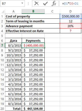
You can go on already blazed way: to computation the internal rate of return, and then multiply the result by 12. But we using the function =XIRR(it returns to the internal percent of return for the schedule of cash flows).

The function arguments:

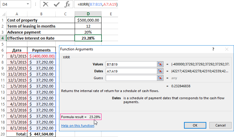
The effective interest on the lease was % to 23. 28%.

Calculation of the effective interest rate on OVDP in Excel

OVDP — domestic government loan bonds. They can be compared with the deposits in a bank. So how exactly the investor gets to a refund of the full amount of invested funds plus additional income as a percentage. The guarantor of the safety of funds is the National Bank.

The effective interest allows estimate to the real income, because it takes into account to capitalization of interest. For example, «acquire» one-year bonds in the sum of 50 000 at 17%. To calculate your income, using the function =FV():

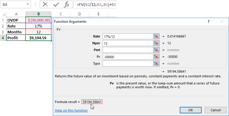
Suppose that the interest to capitalize by monthly. Therefore, we divide 17% by 12. The result as a decimal insertion we put in the field «Bet». In the «Nper» we enter to the number of periods of compounding. Monthly fixed payments we will not get, so the field «Pmt» leaving free. In the column «Pv» we put the deposit invested funds with the sign «-».

Download calculation effective interest rates in Excel

In the window, we immediately see to the sum, which you can get for the bonds in the end of the term. This is the monetary value of accrued compound interest.

What is the “RATE Function”?

The RATE function is a financial function in Excel that calculates the interest rate per period of an annuity. The function is used to calculate the periodic interest rate, which can then be multiplied as required to calculate the annual interest rate. The function calculates by iteration.

The function can be used to calculate the interest rate charged by a loan or offered by an investment for a given period. The RATE function’s output can help decide whether to borrow at a particular interest rate or invest in a security, such as bonds, at the rate of return offered.

Key Learning Points

• The RATE function is a financial function in Excel used for calculating the interest rate of a loan or an investment for a given period. The function can be applied to loans to calculate the percentage of interest charged or to investments to calculate the percentage of return offered
• While interest rate can also be calculated without the RATE function, it makes the calculation more efficient
• The RATE function gives its output through trial and error. If the results do not converge within 20 iterations, it presents a #NUM! error in Excel
• The function returns a #Value! error if any of the supplied arguments are non-numeric

Syntax

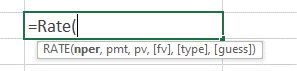
The syntax for the RATE function is shown as:

Rate(nper, pmt, pv, [fv], [type], [guess]

The syntax includes the following arguments:

• Nper represents the number of payment periods for which the interest rate is being calculated. The periods can be in months, quarters, or years. The output of the RATE function (the interest rate) is based on the period included in this argument. The annualized return can be calculated from the period return.
• Pmt is the amount of payment in each period. This number must be constant over the loan’s/investment’s life. If Pmt is omitted, the FV value should be entered.
• PV is the present value of the future payments. For example, if it is a loan, the PV is the amount borrowed. If it is an investment, the PV is the amount invested today.

Optional Arguments

• FV is the future value or the cash balance after the last payment is made. If it is a loan, the FV will be 0. If it is an investment, the FV will be the desired amount of cash flow resulting from the payments. If FV is omitted, it is assumed to be 0.
• Type indicates the payment due dates. If the payment is to be made at the end of each period, the type is 0. If payment is due at the beginning, the type is 1.
• Guess is a guess of what the interest rate is likely to be. If omitted, the rate is assumed to be 10%.

Important Points about the RATE Function

• The RATE function calculates the rate with an iterative process (trial and error). It will return a #NUM! error value if the results do not converge within 20 iterations. The guess provides a starting point for the rate function to converge an answer sooner before reaching 20 iterations. If RATE does not converge, try and input other values in the guess argument.
• #NUM! error value may also be returned due to errors related to cash flow conventions. Typically, cash outflows are input with a negative sign.
• #VALUE! error happens if any of the arguments are non-numeric.
• The Nper argument should be consistent with the payment. For example, if it is a 5-year loan with an interest payment of 200 per month, the NPER should 60 (5 years x 12 months). Also, the units used for Nper and guess should be consistent.
• The output given by the RATE function depends on the period input for loan payments. For example, if the NPER is 12 and the input in PMT is monthly payments, the RATE function’s output will be a monthly interest rate. If you want the annual interest rate, you need to multiply the monthly rate by 12.

Example 1:

Based on the information below, we have been asked to calculate the interest rate for this loan using Excel’s RATE function. Download this free rate function workout from our blog and practice yourself.

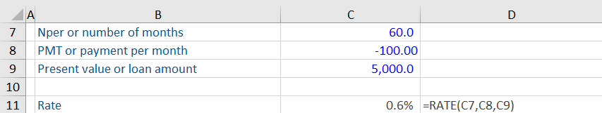
The RATE function has calculated the interest rate for this loan as 0.6%. The payment per month is entered as a negative number to reflect a cash outflow. This output is the monthly interest rate as the Nper and payments are monthly. If you want the annual interest rate, you need to multiply this output by 12.

Example 2:

Calculate the yield to maturity or the return rate offered by the bond below. Coupon payments are made at the end of each year.

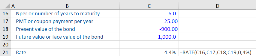
The bond gives an annualized return of 4.4%. Notice we have also included the optional arguments, including a guess of the interest rate as 4%. The present value is a negative number as investing in the bond today will lead to a cash outflow. Investing in a bond is different from taking a loan, where first there is a cash inflow, followed by outflows towards interest and principal repayment. In a bond, in the beginning, there is a cash outflow (the investment), followed by cash inflows (interest payments and eventually the original investment).