Interest payments in excel

Excel for Microsoft 365 Excel for Microsoft 365 for Mac Excel for the web Excel 2021 Excel 2021 for Mac Excel 2019 Excel 2019 for Mac Excel 2016 Excel 2016 for Mac Excel 2013 Excel 2010 Excel for Mac 2011 Excel Mobile More…Less

Managing personal finances can be a challenge, especially when trying to plan your payments and savings. Excel formulas and budgeting templates can help you calculate the future value of your debts and investments, making it easier to figure out how long it will take for you to reach your goals. Use the following functions:

PMT calculates the payment for a loan based on constant payments and a constant interest rate.
NPER calculates the number of payment periods for an investment based on regular, constant payments and a constant interest rate.
PV returns the present value of an investment. The present value is the total amount that a series of future payments is worth now.
FV returns the future value of an investment based on periodic, constant payments and a constant interest rate.

Figure out the monthly payments to pay off a credit card debt

Assume that the balance due is $5,400 at a 17% annual interest rate. Nothing else will be purchased on the card while the debt is being paid off.

Using the function PMT(rate,NPER,PV)

=PMT(17%/12,2*12,5400)

the result is a monthly payment of $266.99 to pay the debt off in two years.

The rate argument is the interest rate per period for the loan. For example, in this formula the 17% annual interest rate is divided by 12, the number of months in a year.
The NPER argument of 2*12 is the total number of payment periods for the loan.
The PV or present value argument is 5400.

Figure out monthly mortgage payments

Imagine a $180,000 home at 5% interest, with a 30-year mortgage.

Using the function PMT(rate,NPER,PV)

=PMT(5%/12,30*12,180000)

the result is a monthly payment (not including insurance and taxes) of $966.28.

The rate argument is 5% divided by the 12 months in a year.
The NPER argument is 30*12 for a 30 year mortgage with 12 monthly payments made each year.
The PV argument is 180000 (the present value of the loan).

Find out how to save each month for a dream vacation

You’d like to save for a vacation three years from now that will cost $8,500. The annual interest rate for saving is 1.5%.

Using the function PMT(rate,NPER,PV,FV)

=PMT(1.5%/12,3*12,0,8500)

to save $8,500 in three years would require a savings of $230.99 each month for three years.

The rate argument is 1.5% divided by 12, the number of months in a year.
The NPER argument is 3*12 for twelve monthly payments over three years.
The PV (present value) is 0 because the account is starting from zero.
The FV (future value) that you want to save is $8,500.

Now imagine that you are saving for an $8,500 vacation over three years, and wonder how much you would need to deposit in your account to keep monthly savings at $175.00 per month. The PV function will calculate how much of a starting deposit will yield a future value.

Using the function PV(rate,NPER,PMT,FV)

=PV(1.5%/12,3*12,-175,8500)

an initial deposit of $1,969.62 would be required in order to be able to pay $175.00 per month and end up with $8500 in three years.

The rate argument is 1.5%/12.
The NPER argument is 3*12 (or twelve monthly payments for three years).
The PMT is -175 (you would pay $175 per month).
The FV (future value) is 8500.

Find out how long it will take to pay off a personal loan

Imagine that you have a $2,500 personal loan, and have agreed to pay $150 a month at 3% annual interest.

Using the function NPER(rate,PMT,PV)

=NPER(3%/12,-150,2500)

it would take 17 months and some days to pay off the loan.

The rate argument is 3%/12 monthly payments per year.
The PMT argument is -150.
The PV (present value) argument is 2500.

Figure out a down payment

Say that you’d like to buy a $19,000 car at a 2.9% interest rate over three years. You want to keep the monthly payments at $350 a month, so you need to figure out your down payment. In this formula the result of the PV function is the loan amount, which is then subtracted from the purchase price to get the down payment.

Using the function PV(rate,NPER,PMT)

=19000-PV(2.9%/12, 3*12,-350)

the down payment required would be $6,946.48

The $19,000 purchase price is listed first in the formula. The result of the PV function will be subtracted from the purchase price.
The rate argument is 2.9% divided by 12.
The NPER argument is 3*12 (or twelve monthly payments over three years).
The PMT is -350 (you would pay $350 per month).

See how much your savings will add up to over time

Starting with $500 in your account, how much will you have in 10 months if you deposit $200 a month at 1.5% interest?

Using the function FV(rate,NPER,PMT,PV)

=FV(1.5%/12,10,-200,-500)

in 10 months you would have $2,517.57 in savings.

The rate argument is 1.5%/12.
The NPER argument is 10 (months).
The PMT argument is -200.
The PV (present value) argument is -500.

Video

You can copy and paste cells A1 through B4 into another part of the spreadsheet in order to evaluate the changes made by different interest rates and terms without losing your original formula and result.

Thanks for submitting a tip for review!

Interest rates are subject to change. Make sure you read the fine print on your interest agreement before you calculate your interest.

About This Article

Article SummaryX

1. Label rows for Principal, Interest, Periods, and Payment.
2. Enter total value in the Principal row.
3. Enter the interest rate into the Interest row.
4. Enter the amount of remaining payments in the Periods row.
5. Click the first blank cell in the Payments row.
6. Type » =IPMT(B2, 1, B3, B1)» into the cell.
7. Press Enter.

Did this summary help you?

Thanks to all authors for creating a page that has been read 502,521 times.

Is this article up to date?

Источник

Excel — is the versatile analytical and computational tool that is often used by lenders (banks, investors, etc.) and borrowers (businessmen, companies, private persons, etc.).

Quickly navigate in the intricate formulas, calculate to interest, payouts, overpayment to allow Microsoft Excel program functions.

How to calculate credit payments in Excel

Monthly payments depend on the loan repayment scheme. There are annuity and differentiated payments:

The annuity assumes that the client makes each month the same amount.
When the differentiated scheme of repayment of debt before the financial organization interest is charged on the balance of the loan amount. Therefore, the monthly payments will be reduced.

Increasingly used annuity: it`s more profitable for the bank, and it is more convenient for the majority of customers.

The calculation of annuity payments on the loan in Excel

The monthly annuity payment is calculated as follows:

S = C * V

where:

S – sum, is the payment amount on the loan;
C – coefficient, is the annuity payment rate;
V – is the value of the loan.

The annuity factor Formula:

С = (i * (1 + i) ^ n) / ((1 + i) ^ n-1)

where is i – the interest rate for the month, the result of dividing the annual rate by 12;
n – is the loan term in months.

There is a special feature in Excel which said to the annuity payments. This is: =PMT().

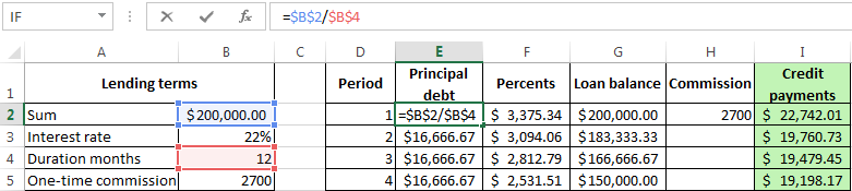
Fill in the input data for calculating the monthly payments on the credit. This is loan amount, interest and term.
To make the repayment schedule. It`s empty till.
In the first cell of the column «Credit payments», introduced the formula of the calculating the loan annuity payments in Excel: =PMT($B$3/12,$B$4,$B$2). To fix the cells, are used to the absolute links. In the formula may be administered directly to the numbers and not the reference cell data. Then it will have the following form: =PMT(18%/12,36,100000).

PMT.

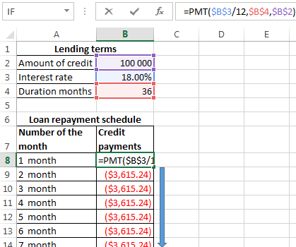
The cells turned into red, because we’ll give these money to the bank and to lose the money.

The calculation of payments in Excel for the differentiated scheme of repayment

The differentiated payment method implies that:

the principal amount is distributed over the period of payment in the equal installments;
the loan interest accrued on the balance.

The formula for the calculating to the differential payment:

DP = NEO / (PP + PS * NEO)

where:

DP – is the monthly payment on the loan;
NEO – is the loan balance;
PP – the number of remaining until the end of the repayment period;
PS – is the interest rate per month (the annual rate divided by 12).

Draw up the schedule for repayment of the previous loan on the differentiated scheme.

The input dates are the same:

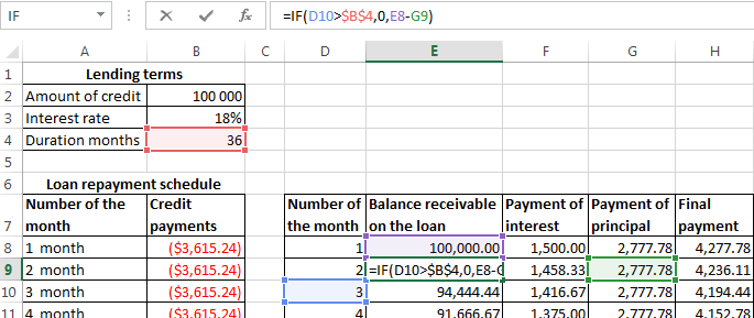
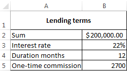
Lending terms
Amount of credit	$100 000
Interest rate	18%
Duration months	36

To make the schedule of repayment of the loan:

Number of the month	Balance receivable on the loan	Payment of interest	Payment of principal	Final payment
1 month

Balance receivable on the loan: in the first month it is equal to the entire amount =$B$2. In the second one and in the subsequent ones — calculated by the formula: =IF(D10>$B$4,0,E8-G9). Where is:

D10 – the number of the current period;
$B$4 – is the term of the loan;
E8 – is the balance of the loan in the previous period;
G9 — is the principal debt in the previous period.

Payment of interest: the balance of the loan in the current period multiplied by the monthly interest rate / 12 months: =E9*($B$3/12).

Payment of principal: the amount of the loan divided by the period: =IF(D9<=$B$4,$B$2/$B$4,0).

Final payment: the sum of «the interest» and «the main debt» in the current period: =F8+G8.

We substitute to the formulas in the corresponding columns. Copy them to the entire table.

To compare the overpayment on the annuity and the differentiated scheme of the repayment on credit:

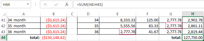
The red figure – is the annuity (was taken 100 000 rubles), the black one – is the differentiated way.

Interest calculation formula for loans in Excel

The calculation of interest on the loan in Excel and calculate the effective interest rate, with the following information on the bank offers credit:

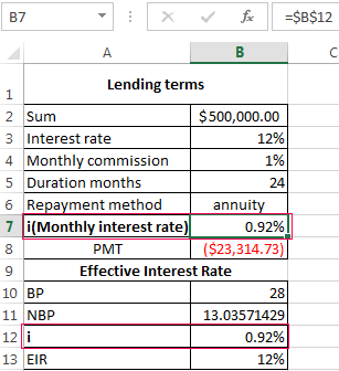
We carry out interest calculation on loan and calculate the effective interest rate with the following information on the bank offers credit.

Fill in the table type:

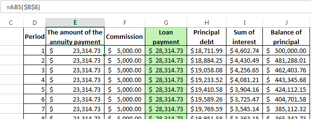
The commission is taken monthly from the whole sum. The total loan payment — this is the annuity payment plus the commission. The sum of the main debt and the sum of interest – there are components parts of the annuity payment.

The principal amount = the annuity payment – the interest.

The sum of interest = the remaining debt * the monthly interest rate.

The balance of principal = the residue of the previous period – the sum of the principal debt in the previous period.

Based on the table of monthly payments, calculate the effective interest rate:

took the credit 500 000 rubles;
returned to the bank — 684 881. 67 rubles (the sum of all payments on the loan);
the overpayment was 184 881. 67 rubles;
the interest rate — 184 881 67/500 000 * 100, or 37%.
the harmless commission of 1% was cost for the borrower so expensive.

The effective interest rate of the loan without the commission will be 13%. The counting is carried out in the same way.

The calculation of effective interest rate in Excel

According to the law about the consumer credit for the calculation of the effective interest rate now is applied the new formula. EIR (Effective Interest Rate) is defined in percentage of up to the third decimal place according to the following formula:

EIR = i * CHBP * 100;
where is i — the interest rate of the base period;
NBP — the number of base periods in a calendar year.

Take for example the following dates on the loan:

For calculating of the effective interest rate is necessary to make a payment schedule (see the order above).

It is necessary to determine the base period (BP). The law states that this is the standard time interval, which is found in most of the repayment schedule. Example BP = 28 days.

Then we find NBP: 365/28 = 13.

Now you can find the interest rate of the base period:

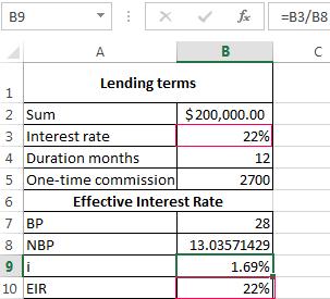
We have all the necessary dates — substitute them in the EIR formula: =B9*B8

To obtain the percentages in Excel, you do not need to multiple by 100. It is enough to set for the cell with the result to the percentage format.

EIR for the new formula is coincided with the annual interest rate on the loan.

Download credit calculator in Excel

Thus, for calculating the annuity payments on the loan is used the simplest function PLT. As you can see, the differentiated way of repayment is a bit more complicated.

Источник

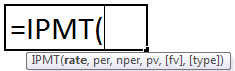
The IPMT function in Excel calculates the interest paid on a given loan where the interest and periodic payments are constant. It is a built-in function in Excel and a type of financial function. This function calculates the interest portion for the payment done for a given period.

For example, suppose the loan amount is $20,000, which needs to be paid in 5 years. The interest rate is 5% per year, and the loan payment needs to be made at the end of every month. Therefore, we need to calculate the interest payments during the first month.

In such a scenario, we can use the IPMT function. Therefore, the IPMT formula will be as follows:

IPMT( 2%/12, 1, 60, 1*12, 20000)

IPMT = $388

So, the calculated IPMT Excel value is $388.

IPMT Function in Excel
- Syntax
- How to use the IPMT Function in Excel? (Examples)
  - Example #1
  - Example #2
  - Example #3
- Things to Remember
- Recommended Articles

Syntax

Compulsory Parameters:

Interest rate: An interest rate for the investment.
Period: Period or duration to calculate the interest rate. It is always a number between 1 and a number of payments.
Number_payments: Payment is a number of payments in the duration.
PV: PV is the present value used as a value of payments.

Optional Parameters:

[FV]: FV is optional here. It is the future value. For example, if you receive a loan, then this is the final payment at the end. Therefore, it will assume 0 as FV.
[Type]: Type is optional here. It indicates that the payments are due. There are two types of parameters for the type.
0: It is used if payments are due at the end of the period, and it automatically defaults.
1: It is used if payments are due at the beginning of the period.

How to use the IPMT Function in Excel? (Examples)

You can download this IPMT Function Excel Template here – IPMT Function Excel Template

Example #1

This first example returns the interest payment for an $8,000 investment that earns 7.5% annually for 2 years. The interest payment is calculated for the 6th month, and payments are due at the end of each month.

=IPMT(7.5%/12, 6, 2*12, 8000).

So, the calculated IPMT value is $40.19.

Example #2

This next example returns the interest payment for a $10,000 investment that earns 5% annually for 4 years. The interest payment is calculated for the 30th week, and payments are due at the beginning of each week.

=IPMT(5%/52, 30, 4*52, 10000, 0 ,1).

So, the calculated IPMT Excel value is $8.38.

Example #3

This next example returns the interest payment for a $6,500 investment that earns 5.25% annually for 10 years. The interest payment is calculated for the 4^th year, and payments are due at the end of each year.

IPMT function as worksheet function:

=IPMT(5.25%/1, 4, 10*1, 6500).

So, the calculated IPMT value is $27.89.

Things to Remember

Below are a few error details in the IPMT function as the wrong argument will be passed in the functions.

Error handling #NUM!: If per value is < 0 or > the value of nper then IPMT function through a #NUM error.
Error handling #VALUE!:#VALUE! Error in Excel represents that the reference cell the user has either entered an incorrect formula or used a wrong data type (mostly numerical data). Sometimes, it is difficult to identify the kind of mistake behind this error.read more IPMT function through a #VALUE! Error when any non-numeric value has been passed in the IPMT formula.

See also

Need more help?

Want more options?