Inserting formulas to excel - Word и Excel - помощь в работе с программами

Create a simple formula in Excel

Excel for Microsoft 365 Excel for Microsoft 365 for Mac Excel 2021 Excel 2021 for Mac Excel 2019 Excel 2019 for Mac Excel 2016 Excel 2016 for Mac Excel 2013 Excel 2010 Excel 2007 Excel for Mac 2011 More…Less

You can create a simple formula to add, subtract, multiply or divide values in your worksheet. Simple formulas always start with an equal sign (=), followed by constants that are numeric values and calculation operators such as plus (+), minus (—), asterisk(*), or forward slash (/) signs.

Let’s take an example of a simple formula.

On the worksheet, click the cell in which you want to enter the formula.
Type the = (equal sign) followed by the constants and operators (up to 8192 characters) that you want to use in the calculation.

For our example, type =1+1.
Notes:
- Instead of typing the constants into your formula, you can select the cells that contain the values that you want to use and enter the operators in between selecting cells.
- Following the standard order of mathematical operations, multiplication and division is performed before addition and subtraction.
Press Enter (Windows) or Return (Mac).

Let’s take another variation of a simple formula. Type =5+2*3 in another cell and press Enter or Return. Excel multiplies the last two numbers and adds the first number to the result.

Use AutoSum

You can use AutoSum to quickly sum a column or row or numbers. Select a cell next to the numbers you want to sum, click AutoSum on the Home tab, press Enter (Windows) or Return (Mac), and that’s it!

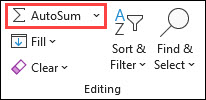
When you click AutoSum, Excel automatically enters a formula (that uses the SUM function) to sum the numbers.

Note: You can also type ALT+= (Windows) or ALT++= (Mac) into a cell, and Excel automatically inserts the SUM function.

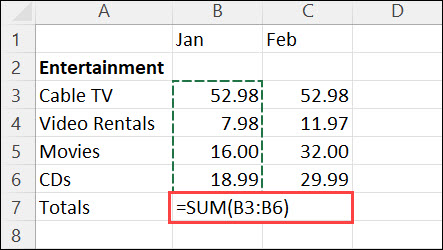
Here’s an example. To add the January numbers in this Entertainment budget, select cell B7, the cell immediately below the column of numbers. Then click AutoSum. A formula appears in cell B7, and Excel highlights the cells you’re totaling.

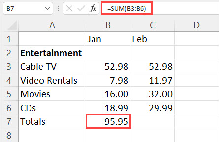
Press Enter to display the result (95.94) in cell B7. You can also see the formula in the formula bar at the top of the Excel window.

Notes:

To sum a column of numbers, select the cell immediately below the last number in the column. To sum a row of numbers, select the cell immediately to the right.
Once you create a formula, you can copy it to other cells instead of typing it over and over. For example, if you copy the formula in cell B7 to cell C7, the formula in C7 automatically adjusts to the new location, and calculates the numbers in C3:C6.
You can also use AutoSum on more than one cell at a time. For example, you could highlight both cell B7 and C7, click AutoSum, and total both columns at the same time.

Copy the example data in the following table, and paste it in cell A1 of a new Excel worksheet. If you need to, you can adjust the column widths to see all the data.

Note: For formulas to show results, select them, press F2, and then press Enter (Windows) or Return (Mac).

Data
2
5
Formula	Description	Result
=A2+A3	Adds the values in cells A1 and A2	=A2+A3
=A2-A3	Subtracts the value in cell A2 from the value in A1	=A2-A3
=A2/A3	Divides the value in cell A1 by the value in A2	=A2/A3
=A2*A3	Multiplies the value in cell A1 times the value in A2	=A2*A3
=A2^A3	Raises the value in cell A1 to the exponential value specified in A2	=A2^A3
Formula	Description	Result
=5+2	Adds 5 and 2	=5+2
=5-2	Subtracts 2 from 5	=5-2
=5/2	Divides 5 by 2	=5/2
=5*2	Multiplies 5 times 2	=5*2
=5^2	Raises 5 to the 2nd power	=5^2

Need more help?

You can always ask an expert in the Excel Tech Community or get support in the Answers community.

Need more help?

Want more options?

Explore subscription benefits, browse training courses, learn how to secure your device, and more.

Communities help you ask and answer questions, give feedback, and hear from experts with rich knowledge.

Источник

Write Basic Formulas in Excel

Formulas are an integral part of Excel. As a new learner of Excel, one does not understand the importance of formulas in Excel. However, all the new learners know plenty of built-in formulas but do not know how to apply them.

In this article, we will show you how to write formulas in Excel and dynamically change them when the referenced cell values are changed automatically.

Write Basic Formulas in Excel
- How to Write/Insert Formulas in Excel?
  - Example #1
  - Example #2
- How to use Built-in Excel Functions?
  - Example #1 – SUM Function
  - Example #2 – AVERAGE Function
- Things to Remember about Inserting Formula in Excel
- Recommended Articles

How to Write/Insert Formulas in Excel?

You can download this Write Formula Excel Template here – Write Formula Excel Template

To write a formula in Excel, you first need to enter the equal sign in the cell where we need to enter the formula. So, the formula always starts with an equal (=) sign.

Example #1

Look at the below data in the Excel worksheet.

We have two numbers in A1 and A2 cells, respectively. So, if we want to add these two numbers in cell A3, we must first open the equal sign in the A3 cell.

Enter the numbers as 525 + 800.

Press the “Enter” key to get the formula equation’s result.

The formula bar shows the formula, not the result of the formula.

As you can see above, we have got the result as 1325 as the summation of the numbers 525 and 800. In the formula bar, we can see how the formula has been applied = 525+800.

Now, we will change the A1 and A2 numbers to 50 and 80, respectively.

Result cell A3 shows the old formula result only. It is where we need to make dynamic cell referenceCell reference in excel is referring the other cells to a cell to use its values or properties. For instance, if we have data in cell A2 and want to use that in cell A1, use =A2 in cell A1, and this will copy the A2 value in A1.read more formulas.

Instead of entering the two cell numbers, give a cell reference only to the formula.

Press the “Enter” key to get the result of this formula.

In the formula bar, we can see the formula as A1 + A2, not the numbers of the A1 and A2 cells. Now, change the numbers of any of the cells. For example, in the A3 cell, it will automatically impact the result.

We have changed the A1 cell number from 50 to 100, and because the A3 cell has the reference of the cells A1 and A2, the A3 cell automatically changed.

Example #2

Now, we have other numbers for the adjacent columns.

We have numbers in four more columns. We need to get the total of these numbers as we did for A1 and A3 cells.

It is where the real power of cell-references formulas is crucial in making the formula dynamic. For example, copy cell A3, which has already applied the formula A1 + A2, and paste it to the next cell, B3.

Look at the result in cell B3. The formula bar says the formula as B1 + B2 instead of A1 + A2.

When we copied and pasted the A3 cell, the formula cell, we moved one column to the right. But in the same row, we have passed the formula. Because we moved one column to the right in the same row-column reference or header value, “A” has been changed to “B,” but row numbers 1 and 2 remain the same.

Copy and paste the formula to other cells to get the total in all the cells.

How to use Built-in Excel Functions?

Example #1 – SUM Function

We have plenty of built-in functions in Excel according to the requirements and situations we can use. For example, look at the below data in Excel.

We have numbers from the A1 to E5 range of cells. In the B7 cell, we need the total sum of these numbers. Adding individual cell references and entering each cell reference one by one consumes a lot of time, so putting an equal sign open SUM function in excelThe SUM function in excel adds the numerical values in a range of cells. Being categorized under the Math and Trigonometry function, it is entered by typing “=SUM” followed by the values to be summed. The values supplied to the function can be numbers, cell references or ranges.read more.

Select the range of cells from A1 to E5 and close the bracket.

Press the “Enter” key to get the total numbers from A1 to E5.

In just a fraction of seconds, we got the total numbers. In the formula bar, we can see the formula as =SUM(A1: E5).

Example #2 – AVERAGE Function

Assume you have students” every subject score, and you need to find the student’s average score. It is possible to find an average score in a fraction of seconds. For example, look at the below data.

Open AVERAGE function in the H2 cell first.

Select the range of cells reference as B2 to G2 because for the student “Amit,” all the subject scores are in this range only.

Press the “Enter” key to get the average student “Amit.”

So, the student “Amit” average score is 79.

Now, drag formula cell H2 to the below cells to get the average of other students.

Things to Remember about Inserting Formula in Excel

The formula should always start with an equal sign. We can also start with a PLUS or MINUS sign but not recommended.
While doing calculations, we need to remember BODMAS’s basic Maths rules.
We must always use built-in functions in Excel.

How to Insert Formulas in Excel?

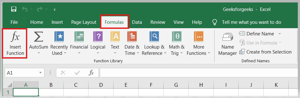
This horizontal menu, shown below, in more recent versions of Excel allows you to find and insert Excel formulas into specific cells of your spreadsheet. On the Formulas tab, you can find all available Excel functions in the Function Library:

The more you use Excel formulas, the easier it will be to remember and perform them manually. Excel has over 400 functions, and the number is increasing from version to version. The formulas can be inserted into Excel using the following method:

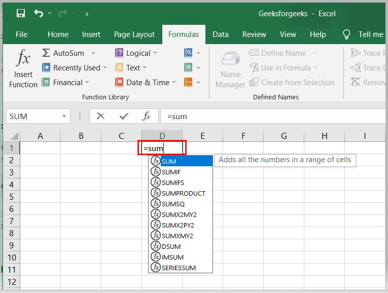
1. Simple insertion of the formula(Typing a formula in the cell):

Typing a formula into a cell or the formula bar is the simplest way to insert basic Excel formulas. Typically, the process begins with typing an equal sign followed by the name of an Excel function. Excel is quite intelligent in that it displays a pop-up function hint when you begin typing the name of the function.

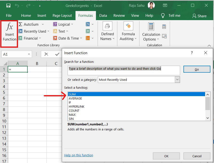
2. Using the Insert Function option on the Formulas Tab:

If you want complete control over your function insertion, use the Excel Insert Function dialogue box. To do so, go to the Formulas tab and select the first menu, Insert Function. All the functions will be available in the dialogue box.

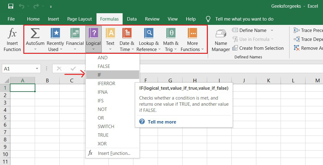
3. Choosing a Formula from One of the Formula Groups in the Formula Tab:

This option is for those who want to quickly dive into their favorite functions. Navigate to the Formulas tab and select your preferred group to access this menu. Click to reveal a sub-menu containing a list of functions. You can then choose your preference. If your preferred group isn’t on the tab, click the More Functions option — it’s most likely hidden there.

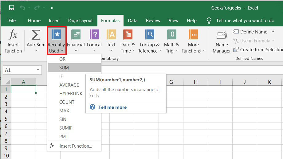
4. Use Recently Used Tabs for Quick Insertion:

If retyping your most recent formula becomes tedious, use the Recently Used menu. It’s on the Formulas tab, the third menu option after AutoSum.

Basic Excel Formulas and Functions:

1. SUM:

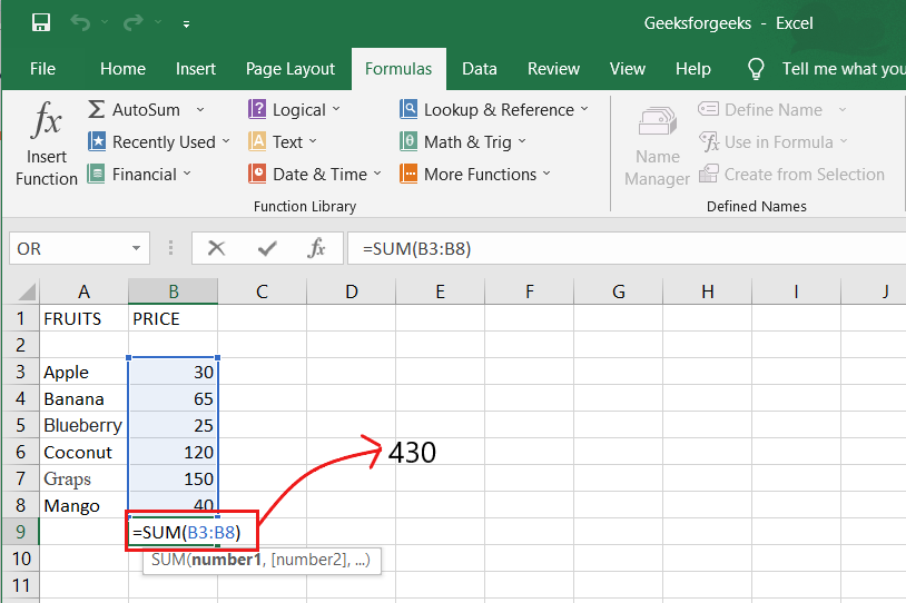
The SUM formula in Excel is one of the most fundamental formulas you can use in a spreadsheet, allowing you to calculate the sum (or total) of two or more values. To use the SUM formula, enter the values you want to add together in the following format: =SUM(value 1, value 2,…..).

Example: In the below example to calculate the sum of price of all the fruits, in B9 cell type =SUM(B3:B8). this will calculate the sum of B3, B4, B5, B6, B7, B8 Press “Enter,” and the cell will produce the sum: 430.

2. SUBTRACTION:

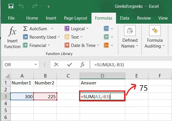
To use the subtraction formula in Excel, enter the cells you want to subtract in the format =SUM (A1, -B1). This will subtract a cell from the SUM formula by appending a negative sign before the cell being subtracted.

For example, if A3 was 300 and B3 was 225, =SUM(A1, -B1) would perform 300 + -225, returning a value of 75 in D3 cell.

3. MULTIPLICATION:

In Excel, enter the cells to be multiplied in the format =A3*B3 to perform the multiplication formula. An asterisk is used in this formula to multiply cell A3 by cell B3.

For example, if A3 was 300 and B3 was 225, =A1*B1 would return a value of 67500.

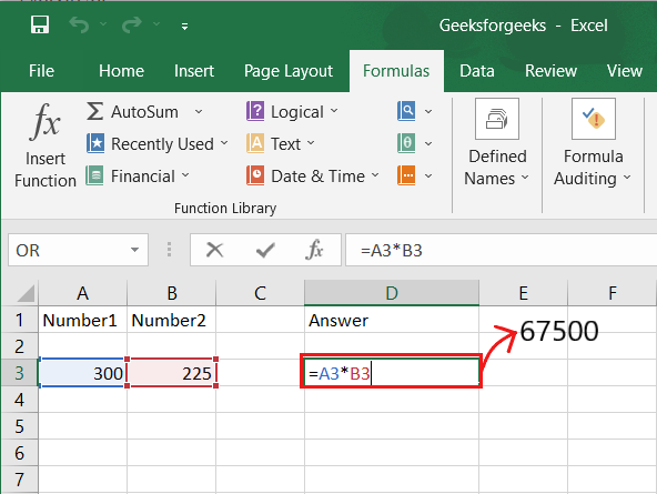
Highlight an empty cell in an Excel spreadsheet to multiply two or more values. Then, in the format =A1*B1…, enter the values or cells you want to multiply together. The asterisk effectively multiplies each value in the formula.

To return your desired product, press Enter. Take a look at the screenshot above to see how this looks.

4. DIVISION:

To use the division formula in Excel, enter the dividing cells in the format =A3/B3. This formula divides cell A3 by cell B3 with a forward slash, “/.”

For example, if A3 was 300 and B3 was 225, =A3/B3 would return a decimal value of 1.333333333.

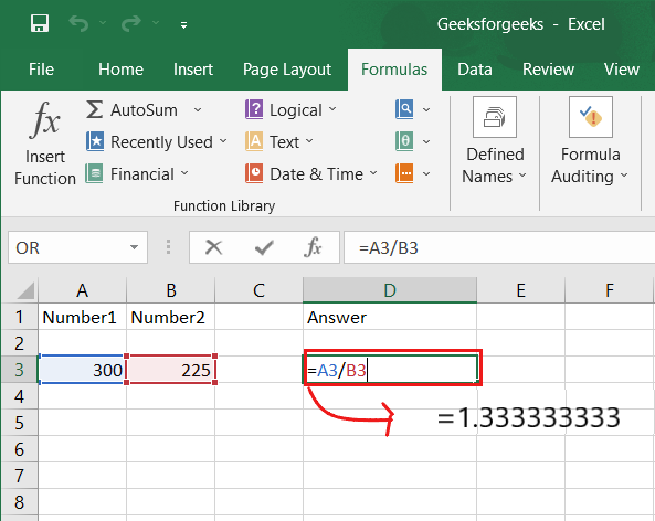
Division in Excel is one of the most basic functions available. To do so, highlight an empty cell, enter an equals sign, “=,” and then the two (or more) values you want to divide, separated by a forward slash, “/.” The output should look like this: =A3/B3, as shown in the screenshot above.

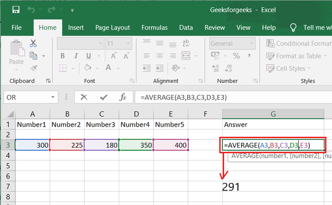
5. AVERAGE:

The AVERAGE function finds an average or arithmetic mean of numbers. to find the average of the numbers type = AVERAGE(A3.B3,C3….) and press ‘Enter’ it will produce average of the numbers in the cell.

For example, if A3 was 300, B3 was 225, C3 was 180, D3 was 350, E3 is 400 then =AVERAGE(A3,B3,C3,D3,E3) will produce 291.

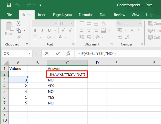
6. IF formula:

In Excel, the IF formula is denoted as =IF(logical test, value if true, value if false). This lets you enter a text value into a cell “if” something else in your spreadsheet is true or false.

For example, You may need to know which values in column A are greater than three. Using the =IF formula, you can quickly have Excel auto-populate a “yes” for each cell with a value greater than 3 and a “no” for each cell with a value less than 3.

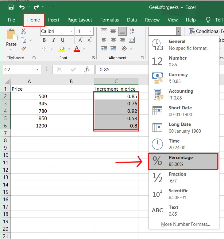
7. PERCENTAGE:

To use the percentage formula in Excel, enter the cells you want to calculate the percentage for in the format =A1/B1. To convert the decimal value to a percentage, select the cell, click the Home tab, and then select “Percentage” from the numbers dropdown.

There isn’t a specific Excel “formula” for percentages, but Excel makes it simple to convert the value of any cell into a percentage so you don’t have to calculate and reenter the numbers yourself.

The basic setting for converting a cell’s value to a percentage is found on the Home tab of Excel. Select this tab, highlight the cell(s) you want to convert to a percentage, and then select Conditional Formatting from the dropdown menu (this menu button might say “General” at first). Then, from the list of options that appears, choose “Percentage.” This will convert the value of each highlighted cell into a percentage. This feature can be found further down.

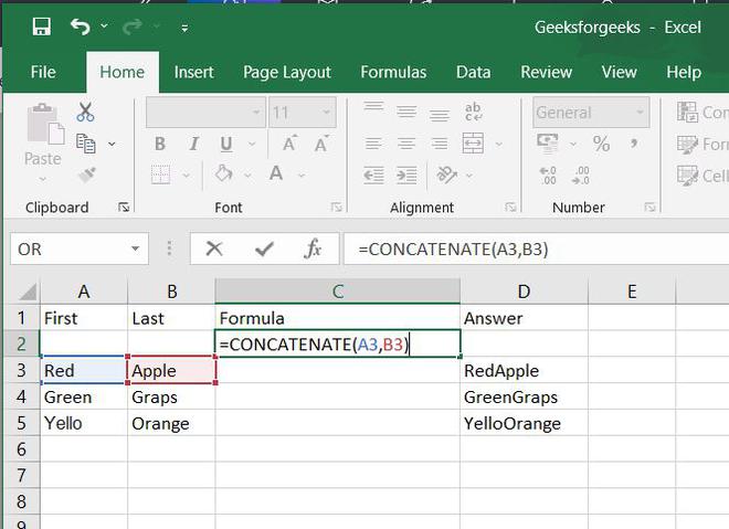
8. CONCATENATE:

CONCATENATE is a useful formula that combines values from multiple cells into the same cell.

For example , =CONCATENATE(A3,B3) will combine Red and Apple to produce RedApple.

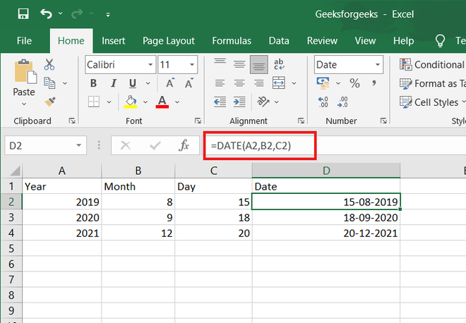
9. DATE:

DATE is the Excel DATE formula =DATE(year, month, day). This formula will return a date corresponding to the values entered in the parentheses, including values referred to from other cells.. For example, if A2 was 2019, B2 was 8, and C1 was 15, =DATE(A1,B1,C1) would return 15-08-2019.

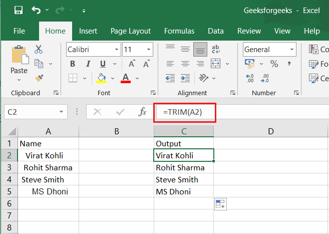
10. TRIM:

The TRIM formula in Excel is denoted =TRIM(text). This formula will remove any spaces that have been entered before and after the text in the cell. For example, if A2 includes the name ” Virat Kohli” with unwanted spaces before the first name, =TRIM(A2) would return “Virat Kohli” with no spaces in a new cell.

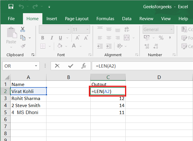
11. LEN:

LEN is the function to count the number of characters in a specific cell when you want to know the number of characters in that cell. =LEN(text) is the formula for this. Please keep in mind that the LEN function in Excel counts all characters, including spaces:

For example,=LEN(A2), returns the total length of the character in cell A2 including spaces.

Источник

Microsoft Excel is a powerful spreadsheet that lets you manage and analyze a large amount of data. You can carry out simple as well as complicated calculations in the most efficient manner. Microsoft Excel is made up of individual cells consisting of rows and columns. Rows are numbered, whereas columns are lettered. Once you have entered the desired values in the cells, it becomes pretty easy to carry out the calculations manually or automatically. You can add, subtract, multiply, and divide in Microsoft Excel by simply using the basic operators such as +, -, *, /. To calculate or analyze a large amount of data or numbers, you can use the built-in functions such as sum, count, average, max, min, and so on.

Basic Calculations in Excel – Addition, Subtraction, Multiplication, Division

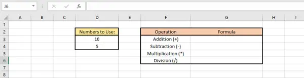
As mentioned earlier, you need to make use of the basic operators like +, -, *, / here. All you need to remember is that all the formulas need to start with a (=) sign. In the Excel sheet below, in the first table, you can see two numbers 10 and 5, which is our data. In the other table, you can see the operations to be carried out by applying appropriate formulas.

Formulas can contain cell references, ranges of cell references, operators, and constants. Let us see how this is done.

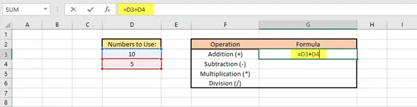
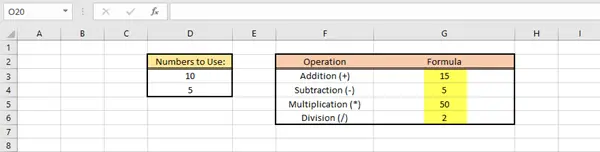
To Add, select cell G3, type =D3+D4, and then press Enter. The answer will automatically be displayed in the cell G3.
To Subtract, select cell G4, type =D3-D4, and then press Enter. The answer will automatically be displayed in the cell G3.
To Multiply, select cell G4, type =D3*D4, and then press Enter. The answer will automatically be displayed in the cell G4.
To Divide, select cell G5, type =D3/D4, and then press Enter. The answer will automatically be displayed in the cell G5.

Quite simple and easy, right?

TIP: This post will help you if Excel Formulas are not updating automatically.

How to insert & use Functions in Excel

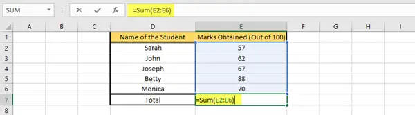
Functions help you perform a variety of mathematical operations, lookup values, calculate date and time, and a lot more. Browse through the Function Library in the Formulas tab to learn more. Now let us see a few examples on how to insert and use functions. The table below displays the name of the student and the marks obtained by each one of them.

To calculate the total marks of all the students, we need to use the Sum Function. There are two ways to so.

1) Select the cell E7, and type =SUM(E2:E6) and then press Enter. The answer will be automatically displayed in cell E7.

2) Click on the cells you want to select, that is, cell E2 to cell E6. In the Formulas tab, under the Function Library group, click on Auto Sum dropdown menu, and then further click on Sum. The correct value will be displayed in cell E7.

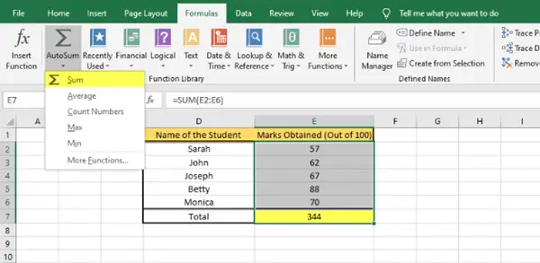
This is how you can calculate the total value from a given set of values by using the Sum Function.

Similarly, you can perform various other functions such as Average, Count, Min, Max, and so on, depending on your requirement.

I hope you found this basic tutorial useful.

Now read: How to calculate the Median in Excel.

Источник

Enter a Formula | Edit a Formula | Operator Precedence | Copy/Paste a Formula | Insert Function

A formula is an expression which calculates the value of a cell. Functions are predefined formulas and are already available in Excel.

Cell A3 below contains a formula which adds the value of cell A2 to the value of cell A1.

Cell A3 below contains the SUM function which calculates the sum of the range A1:A2.

Enter a Formula

To enter a formula, execute the following steps.

1. Select a cell.

2. To let Excel know that you want to enter a formula, type an equal sign (=).

3. For example, type the formula A1+A2.

Tip: instead of typing A1 and A2, simply select cell A1 and cell A2.

4. Change the value of cell A1 to 3.

Excel automatically recalculates the value of cell A3. This is one of Excel’s most powerful features!

Edit a Formula

When you select a cell, Excel shows the value or formula of the cell in the formula bar.

1. To edit a formula, click in the formula bar and change the formula.

2. Press Enter.

Operator Precedence

Excel uses a default order in which calculations occur. If a part of the formula is in parentheses, that part will be calculated first. It then performs multiplication or division calculations. Once this is complete, Excel will add and subtract the remainder of your formula. See the example below.

First, Excel performs multiplication (A1 * A2). Next, Excel adds the value of cell A3 to this result.

Another example,

First, Excel calculates the part in parentheses (A2+A3). Next, it multiplies this result by the value of cell A1.

Copy/Paste a Formula

When you copy a formula, Excel automatically adjusts the cell references for each new cell the formula is copied to. To understand this, execute the following steps.

1. Enter the formula shown below into cell A4.

2a. Select cell A4, right click, and then click Copy (or press CTRL + c)…

…next, select cell B4, right click, and then click Paste under ‘Paste Options:’ (or press CTRL + v).

2b. You can also drag the formula to cell B4. Select cell A4, click on the lower right corner of cell A4 and drag it across to cell B4. This is much easier and gives the exact same result!

Result. The formula in cell B4 references the values in column B.

Insert Function

Every function has the same structure. For example, SUM(A1:A4). The name of this function is SUM. The part between the brackets (arguments) means we give Excel the range A1:A4 as input. This function adds the values in cells A1, A2, A3 and A4. It’s not easy to remember which function and which arguments to use for each task. Fortunately, the Insert Function feature in Excel helps you with this.

To insert a function, execute the following steps.

1. Select a cell.

2. Click the Insert Function button.

The ‘Insert Function’ dialog box appears.

3. Search for a function or select a function from a category. For example, choose COUNTIF from the Statistical category.

4. Click OK.

The ‘Function Arguments’ dialog box appears.

5. Click in the Range box and select the range A1:C2.

6. Click in the Criteria box and type >5.

7. Click OK.

Result. The COUNTIF function counts the number of cells that are greater than 5.

Note: instead of using the Insert Function feature, simply type =COUNTIF(A1:C2,»>5″). When you arrive at: =COUNTIF( instead of typing A1:C2, simply select the range A1:C2.

Источник

Use AutoSum

Need more help?

Need more help?

Want more options?

Write Basic Formulas in Excel

Table of contents

How to Write/Insert Formulas in Excel?

Example #1

Example #2

How to use Built-in Excel Functions?

Example #1 – SUM Function

Example #2 – AVERAGE Function

Things to Remember about Inserting Formula in Excel

Recommended Articles

How to Insert Formulas in Excel?

1. Simple insertion of the formula(Typing a formula in the cell):

2. Using the Insert Function option on the Formulas Tab:

3. Choosing a Formula from One of the Formula Groups in the Formula Tab:

4. Use Recently Used Tabs for Quick Insertion:

Basic Excel Formulas and Functions:

1. SUM:

2. SUBTRACTION:

3. MULTIPLICATION:

4. DIVISION:

5. AVERAGE:

6. IF formula:

7. PERCENTAGE:

8. CONCATENATE:

9. DATE:

10. TRIM:

11. LEN:

Basic Calculations in Excel – Addition, Subtraction, Multiplication, Division

How to insert & use Functions in Excel

Enter a Formula

Edit a Formula

Operator Precedence

Copy/Paste a Formula

Insert Function