Insert words in excel - Word и Excel - помощь в работе с программами

Содержание

Insert an object in your Excel spreadsheet
Insert Character or Text to Cells
Insert Character or Text to Cells with a Formula
Insert Character or Text to Cells with VBA
Insert an object in your Excel spreadsheet
How to Add Text to the Beginning or End of all Cells in Excel
Method 1: Using the ampersand Operator
Using the ampersand Operator to Add Text to the Beginning of all Cells
Using the ampersand Operator to Add Text to the End of all Cells
Method 2: Using the CONCATENATE Function
Using CONCATENATE to Add Text to the Beginning of all Cells
Using CONCATENATE to Add Text to the End of all Cells
Method 3: Using the Flash Fill Feature
Using Flash Fill to Add Text to the Beginning of all Cells
Using Flash Fill to Add Text to the End of all Cells in a Column
Method 4: Using VBA Code
Using VBA to Add Text to the Beginning of all Cells in a Column
Using VBA to Add Text to the End of all Cells in a Column

Insert an object in your Excel spreadsheet

You can use Object Linking and Embedding (OLE) to include content from other programs, such as Word or Excel.

OLE is supported by many different programs, and OLE is used to make content that is created in one program available in another program. For example, you can insert an Office Word document in an Office Excel workbook. To see what types of content that you can insert, click Object in the Text group on the Insert tab. Only programs that are installed on your computer and that support OLE objects appear in the Object type box.

If you copy information between Excel or any program that supports OLE, such as Word, you can copy the information as either a linked object or an embedded object. The main differences between linked objects and embedded objects are where the data is stored and how the object is updated after you place it in the destination file. Embedded objects are stored in the workbook that they are inserted in, and they are not updated. Linked objects remain as separate files, and they can be updated.

Linked and embedded objects in a document

1. An embedded object has no connection to the source file.

2. A linked object is linked to the source file.

3. The source file updates the linked object.

When to use linked objects

If you want the information in your destination file to be updated when the data in the source file changes, use linked objects.

With a linked object, the original information remains stored in the source file. The destination file displays a representation of the linked information but stores only the location of the original data (and the size if the object is an Excel chart object). The source file must remain available on your computer or network to maintain the link to the original data.

The linked information can be updated automatically if you change the original data in the source file. For example, if you select a paragraph in a Word document and then paste the paragraph as a linked object in an Excel workbook, the information can be updated in Excel if you change the information in your Word document.

When to use embedded objects

If you don’t want to update the copied data when it changes in the source file, use an embedded object. The version of the source is embedded entirely in the workbook. If you copy information as an embedded object, the destination file requires more disk space than if you link the information.

When a user opens the file on another computer, he can view the embedded object without having access to the original data. Because an embedded object has no links to the source file, the object is not updated if you change the original data. To change an embedded object, double-click the object to open and edit it in the source program. The source program (or another program capable of editing the object) must be installed on your computer.

Changing the way that an OLE object is displayed

You can display a linked object or embedded object in a workbook exactly as it appears in the source program or as an icon. If the workbook will be viewed online, and you don’t intend to print the workbook, you can display the object as an icon. This minimizes the amount of display space that the object occupies. Viewers who want to display the information can double-click the icon.

Источник

Insert Character or Text to Cells

This post will guide you how to insert character or text in middle of cells in Excel. How do I add text string or character to each cell of a column or range with a formula in Excel. How to add text to the beginning of all selected cells in Excel. How to add character after the first character of cells in Excel.

Assuming that you have a list of data in range B1:B5 that contain string values and you want to add one character “E” after the first character of string in Cells. You can refer to the following two methods.

Insert Character or Text to Cells with a Formula

To insert the character to cells in Excel, you can use a formula based on the LEFT function and the MID function. Like this:

Type this formula into a blank cell, such as: Cell C1, and press Enter key. And then drag the AutoFill Handle down to other cells to apply this formula.

This formula will inert the character “E” after the first character of string in Cells. And if you want to insert the character or text string after the second or third or N position of the string in Cells, you just need to replace the number 1 in Left function and the number 2 in MID function as 2 and 3. Like below:

Insert Character or Text to Cells with VBA

You can also use an Excel VBA Macro to insert one character or text after the first position of the text string in Cells. Just do the following steps:

#1 open your excel workbook and then click on “Visual Basic” command under DEVELOPER Tab, or just press “ALT+F11” shortcut.

#2 then the “Visual Basic Editor” window will appear.

#3 click “Insert” ->”Module” to create a new module.

#4 paste the below VBA code into the code window. Then clicking “Save” button.

#5 back to the current worksheet, then run the above excel macro. Click Run button.

#6 select one Range that you want to insert one character.

Источник

Insert an object in your Excel spreadsheet

You can use Object Linking and Embedding (OLE) to include content from other programs, such as Word or Excel.

Linked and embedded objects in a document

1. An embedded object has no connection to the source file.

2. A linked object is linked to the source file.

3. The source file updates the linked object.

When to use linked objects

If you want the information in your destination file to be updated when the data in the source file changes, use linked objects.

When to use embedded objects

Changing the way that an OLE object is displayed

Источник

How to Add Text to the Beginning or End of all Cells in Excel

There may be instances where you need to add the same text to all cells in a column. You might need to add a particular title before names in a list, or a particular symbol at the end of the text in every cell.

The good thing is you don’t need to do this manually.

Excel provides some really simple ways in which you can add text to the beginning and/ or end of the text in a range of cells.

In this tutorial we will see 4 ways to do this:

Using the ampersand operator (&)
Using the CONCATENATE function
Using the Flash Fill feature
Using VBA

So let’s get started!

Table of Contents

Method 1: Using the ampersand Operator

An ampersand (&) can be used to easily combine text strings in Excel. Let’s see how you use it to add text at the beginning or end or both in Excel.

Using the ampersand Operator to Add Text to the Beginning of all Cells

The ampersand (&) is an operator that is mainly used to join several text strings into one.

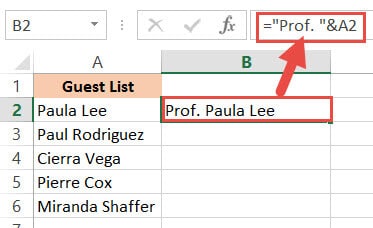
Here’s how you can use it to add text to the beginning of all cells in a range. Let us assume you have the following list of names and want to add the title “Prof.” before every name:

Below are the steps to add a text before a text string in Excel:

Click on the first cell of the column where you want the converted names to appear (B2).
Type equal sign (=), followed by the text “Prof. “, followed by an ampersand (&).
Select the cell containing the first name (A2).
Press the Return Key.
You will notice that the title “Prof.” is added before the first name in the list.
It’s now time to copy this formula to the rest of the cells in the column. Simply double click the fill handle (located at the bottom right of cell B2). Alternatively, you can drag down the fill handle to achieve the same effect.

That’s it, all your cells in column B should now contain the title “Prof.” preceding each name.

Using the ampersand Operator to Add Text to the End of all Cells

Now let us see how to add some text to the end of every name in the dataset. Let us say you want to add the text “(MD)” at the end of every name. In that case, here are the steps you need to follow:

Click on the first cell of the column where you want the converted names to appear (C2 in our case).
Type equal sign (=)
Select the cell containing the first name (B2 in our case).
Next, insert an ampersand (&), followed by the text “ (MD)”.
Press the Return Key.
You will notice that the text “(MD).” added after the first name in the list.
It’s now time to copy this formula to the rest of the cells in the column. Simply double click the fill handle (located at the bottom right of cell C2). Alternatively, you can drag down the fill handle to achieve the same effect.

All your cells in column C should now contain the text “(MD”) at the end of each name.

Method 2: Using the CONCATENATE Function

CONCATENATE is an Excel function that you can use to add text at the beginning and end of the text string.

Let’s see how to use CONCATENATE to do this.

Using CONCATENATE to Add Text to the Beginning of all Cells

The CONCATENATE() function provides the same functionality as the ampersand (&) operator. The only difference is in the way both are used.

The general syntax for the CONCATENATE function is:

Where text1, text2, etc. are substrings that you want to combine together.

Let’s apply the CONCATENATE function to the same dataset as above:

Click on the first cell of the column where you want the converted names to appear (B2).
Type equal sign (=).
Enter the function CONCATENATE, followed by an opening bracket (.
Type the title “Prof. ” in double-quotes, followed by a comma (,).
Select the cell containing the first name (A2)
Place a closing bracket. In our example, your formula should now be: =CONCATENATE(“Prof. “,A2).
Press the Return Key.
You will notice that the title “Prof.” is added before the first name on the list.
It’s now time to copy this formula to the rest of the cells in the column. Simply double click the fill handle (located at the bottom right of cell B2). Alternatively, you can drag down the fill handle to achieve the same effect.

That’s it, all your cells in column B should now contain the title “Prof.” preceding each name.

Using CONCATENATE to Add Text to the End of all Cells

Click on the first cell of the column where you want the converted names to appear (C2 in our example).
Type equal sign (=).
Enter the function CONCATENATE, followed by an opening bracket (.
Select the cell containing the first name (B2 in our example).
Next, insert a comma, followed by the text “ (MD)”.
Place a closing bracket. In our example, your formula should now be: =CONCATENATE(B2,” (MD)”).
Press the Return Key.
You will notice that the text “(MD).” added after the first name in the list.
It’s now time to copy this formula to the rest of the cells in the column. Simply double click the fill handle (located at the bottom right of cell C2).

All your cells in column C should now contain the text “(MD”) at the end of each name.

Notice that since you’re using a formula, your column C depends on columns A and B. So if you make any changes to the original values in column A, they get reflected in column C.

If you decide to only retain the converted names and delete columns A and B, you will get an error, as shown below:

To make sure that this does not happen, it’s best to first convert the formula results to permanent values copying them and pasting them as values in the same column (Right-click and select Paste Options->Values from the Popup menu).

Now you can go ahead and delete columns A and B if you need to.

Method 3: Using the Flash Fill Feature

Flash fill is a relatively new feature that looks at the pattern of what you are trying to achieve and then does it for all the cells in a column.

You can also use Flash fill to so text manipulation as we will see in the following examples.

Using Flash Fill to Add Text to the Beginning of all Cells

The Excel flash fill feature is like a magical button. It is available if you’re on any Excel version from 2013 onwards.

The feature takes advantage of Excel’s pattern recognition capabilities. It basically recognizes a pattern in your data and automatically fills in the other cells of the column with the same pattern for you.

Here’s how you can use Flash Fill to add text to the beginning of all cells in a column:

Click on the first cell of the column where you want the converted names to appear (B2).
Manually type in the text Prof. , followed by the first name of your list.
Press the Return Key.
Click on cell B2 again.
Under the Data tab, click on the Flash Fill button (in the ‘Data Tools’ group). Alternatively, you can just press CTRL+E on your keyboard (Command+E if you’re on a Mac).

This will copy the same pattern to the rest of the cells in the column… in a flash!

Using Flash Fill to Add Text to the End of all Cells in a Column

If you want to add the text “ (MD)” to the end of the names, follow the same steps:

Click on the first cell of the column where you want the converted names to appear (C2).
Manually type in or copy the text from column B2 into C2.
Add the text “(MD)” after that.
Under the Data tab, click on the Flash Fill or press CTRL+E on your keyboard (Command+E if you’re on a Mac).

That’s all, you get every cell filled in with the same pattern!

We especially like this method because it is simple, quick, and easy. Moreover, since it’s formula-free, the results do not depend on the original columns.

So they remain unchanged even if you delete rows A and B!

Method 4: Using VBA Code

And of course, if you’re comfortable with VBA, you can also add text before or after a text string using it.

Using VBA to Add Text to the Beginning of all Cells in a Column

If coding with VBA does not intimidate you then this method can help get your work done quickly too.

Here’s the code we will be using to add the title “Prof. “ to the beginning of all cells in a range. You can select and copy it:

Follow these steps to use the above code:

From the Developer Menu Ribbon, select Visual Basic.
Once your VBA window opens, Click Insert->Module. Now you can start coding. Type or copy-paste the above lines of code into the module window. Your code is now ready to run.
Select the range of cells containing the text you want to convert. Make sure the column next to it is blank because this is where the code will display the results.
Navigate to Developer->Macros-> add_text_to_beginning->Run.

You will now see the converted text next to your selected range of cells.

Note: You can change the text in line 6 from “Prof. ” to whatever text you need to add to the beginning of all cells.

Using VBA to Add Text to the End of all Cells in a Column

Now, what if you want to add text to the end of all the cells, instead of the beginning? This only involves making a tweak to line 6 of the above code. So if you want to add the text “ (MD)” to the end of all cells, change line 6 to:

cell.Offset(0, 1).Value = cell.Value & “ (MD)”

So your full code should now be:

Here’s the final result:

You can now delete the first two columns if you need to. Do remember to keep a backup of your sheet, because the results of VBA code are usually irreversible.

Note: You can change the text in line 6 from “ (MD)” to whatever text you need to add to the end of all cells in the range.

In this tutorial, we showed you four ways in which you can add text to the beginning and/ or end of all cells in a range.

There are plenty of other methods that you can find online too, and all of them work just as well as the ones shown here.

You may feel free to choose whatever method suits you, your requirement, and your version of Excel. In the end, what matters is getting what you need to be done quickly and effectively.

Other Excel tutorials you may like:

Источник

You can use Object Linking and Embedding (OLE) to include content from other programs, such as Word or Excel.

OLE is supported by many different programs, and OLE is used to make content that is created in one program available in another program. For example, you can insert an Office Word document in an Office Excel workbook. To see what types of content that you can insert, click Object in the Text group on the Insert tab. Only programs that are installed on your computer and that support OLE objects appear in the Object type box.

Linked and embedded objects in a document

1. An embedded object has no connection to the source file.

2. A linked object is linked to the source file.

3. The source file updates the linked object.

When to use linked objects

If you want the information in your destination file to be updated when the data in the source file changes, use linked objects.

When to use embedded objects

Changing the way that an OLE object is displayed

Embed an object in a worksheet

Click inside the cell of the spreadsheet where you want to insert the object.
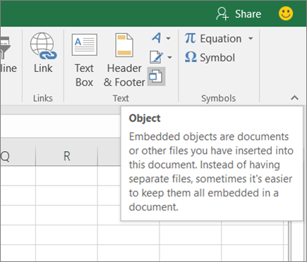
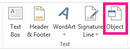
On the Insert tab, in the Text group, click Object .
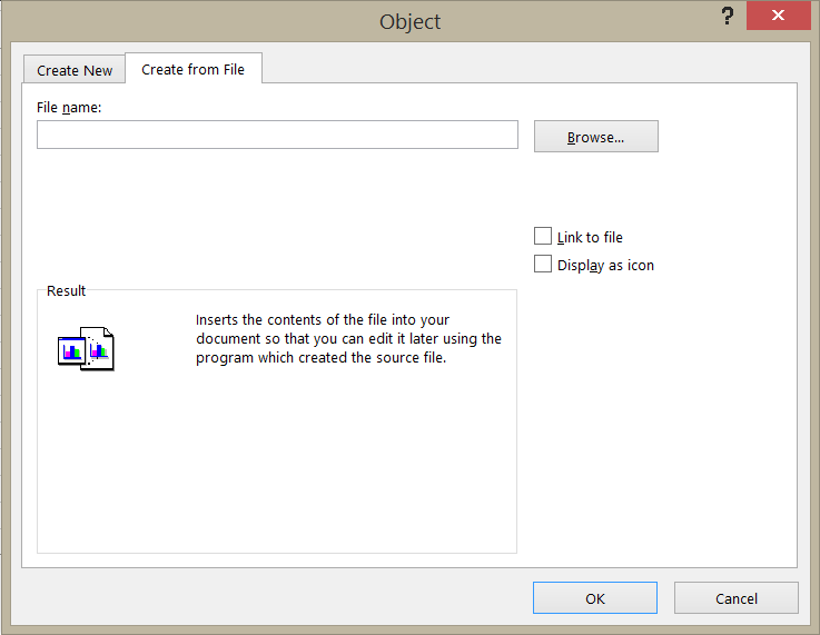
In the Object dialog box, click the Create from File tab.
Click Browse, and select the file you want to insert.
If you want to insert an icon into the spreadsheet instead of show the contents of the file, select the Display as icon check box. If you don’t select any check boxes, Excel shows the first page of the file. In both cases, the complete file opens with a double click. Click OK.

Note: After you add the icon or file, you can drag and drop it anywhere on the worksheet. You can also resize the icon or file by using the resizing handles. To find the handles, click the file or icon one time.

Insert a link to a file

You might want to just add a link to the object rather than fully embedding it. You can do that if your workbook and the object you want to add are both stored on a SharePoint site, a shared network drive, or a similar location, and if the location of the files will remain the same. This is handy if the linked object undergoes changes because the link always opens the most up-to-date document.

Note: If you move the linked file to another location, the link won’t work anymore.

Click inside the cell of the spreadsheet where you want to insert the object.
On the Insert tab, in the Text group, click Object .
Click the Create from File tab.
Click Browse, and then select the file you want to link.
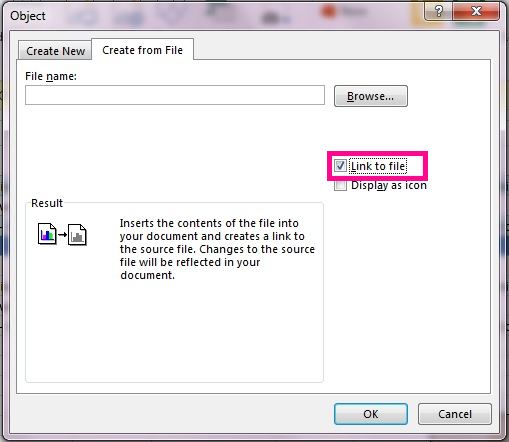
Select the Link to file check box, and click OK.

Create a new object from inside Excel

You can create an entirely new object based on another program without leaving your workbook. For example, if you want to add a more detailed explanation to your chart or table, you can create an embedded document, such as a Word or PowerPoint file, in Excel. You can either set your object to be displayed right in a worksheet or add an icon that opens the file.

Click inside the cell of the spreadsheet where you want to insert the object.
On the Insert tab, in the Text group, click Object .
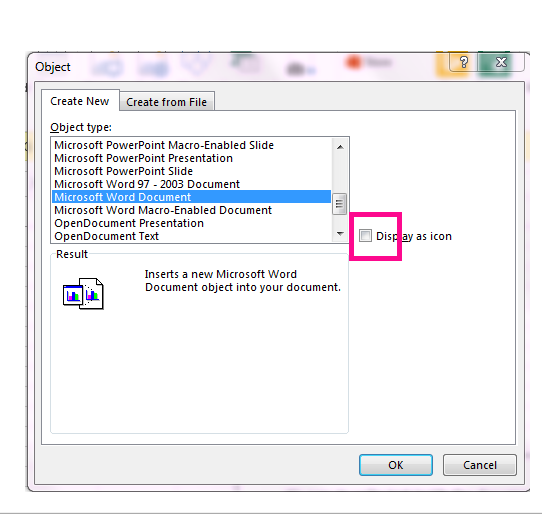
On the Create New tab, select the type of object you want to insert from the list presented. If you want to insert an icon into the spreadsheet instead of the object itself, select the Display as icon check box.
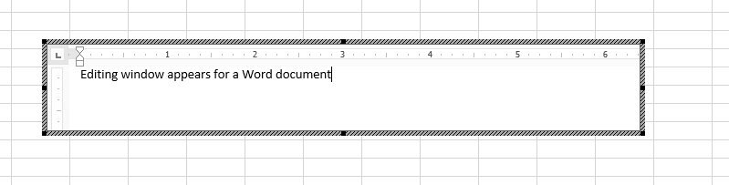
Click OK. Depending on the type of file you are inserting, either a new program window opens or an editing window appears within Excel.
Create the new object you want to insert.

When you’re done, if Excel opened a new program window in which you created the object, you can work directly within it.

When you’re done with your work in the window, you can do other tasks without saving the embedded object. When you close the workbook your new objects will be saved automatically.

Note: After you add the object, you can drag and drop it anywhere on your Excel worksheet. You can also resize the object by using the resizing handles. To find the handles, click the object one time.

Embed an object in a worksheet

Click inside the cell of the spreadsheet where you want to insert the object.
On the Insert tab, in the Text group, click Object.
Click the Create from File tab.
Click Browse, and select the file you want to insert.
If you want to insert an icon into the spreadsheet instead of show the contents of the file, select the Display as icon check box. If you don’t select any check boxes, Excel shows the first page of the file. In both cases, the complete file opens with a double click. Click OK.

Note: After you add the icon or file, you can drag and drop it anywhere on the worksheet. You can also resize the icon or file by using the resizing handles. To find the handles, click the file or icon one time.

Insert a link to a file

Note: If you move the linked file to another location, the link won’t work anymore.

Click inside the cell of the spreadsheet where you want to insert the object.
On the Insert tab, in the Text group, click Object.
Click the Create from File tab.
Click Browse, and then select the file you want to link.
Select the Link to file check box, and click OK.

Create a new object from inside Excel

Click inside the cell of the spreadsheet where you want to insert the object.
On the Insert tab, in the Text group, click Object.
On the Create New tab, select the type of object you want to insert from the list presented. If you want to insert an icon into the spreadsheet instead of the object itself, select the Display as icon check box.
Click OK. Depending on the type of file you are inserting, either a new program window opens or an editing window appears within Excel.
Create the new object you want to insert.

When you’re done, if Excel opened a new program window in which you created the object, you can work directly within it.

When you’re done with your work in the window, you can do other tasks without saving the embedded object. When you close the workbook your new objects will be saved automatically.

Note: After you add the object, you can drag and drop it anywhere on your Excel worksheet. You can also resize the object by using the resizing handles. To find the handles, click the object one time.

Link or embed content from another program by using OLE

You can link or embed all or part of the content from another program.

Create a link to content from another program

Click in the worksheet where you want to place the linked object.
On the Insert tab, in the Text group, click Object.
Click the Create from File tab.
In the File name box, type the name of the file, or click Browse to select from a list.
Select the Link to file check box.
Do one of the following:
- To display the content, clear the Display as icon check box.
- To display an icon, select the Display as icon check box. Optionally, to change the default icon image or label, click Change Icon, and then click the icon that you want from the Icon list, or type a label in the Caption box.
Note: You cannot use the Object command to insert graphics and certain types of files. To insert a graphic or file, on the Insert tab, in the Illustrations group, click Picture.

Embed content from another program

Click in the worksheet where you want to place the embedded object.
On the Insert tab, in the Text group, click Object.
If the document does not already exist, click the Create New tab. In the Object type box, click the type of object that you want to create.

If the document already exists, click the Create from File tab. In the File name box, type the name of the file, or click Browse to select from a list.
Clear the Link to file check box.
Do one of the following:
- To display the content, clear the Display as icon check box.
- To display an icon, select the Display as icon check box. To change the default icon image or label, click Change Icon, and then click the icon that you want from the Icon list, or type a label in the Caption box.

Link or embed partial content from another program

From a program other than Excel, select the information that you want to copy as a linked or embedded object.
On the Home tab, in the Clipboard group, click Copy.
Switch to the worksheet that you want to place the information in, and then click where you want the information to appear.
On the Home tab, in the Clipboard group, click the arrow below Paste, and then click Paste Special.
Do one of the following:
- To paste the information as a linked object, click Paste link.
- To paste the information as an embedded object, click Paste. In the As box, click the entry with the word «object» in its name. For example, if you copied the information from a Word document, click Microsoft Word Document Object.

Change the way that an OLE object is displayed

Right-click the icon or object, point to object typeObject (for example, Document Object), and then click Convert.
Do one of the following:
- To display the content, clear the Display as icon check box.
- To display an icon, select the Display as icon check box. Optionally, you can change the default icon image or label. To do that, click Change Icon, and then click the icon that you want from the Icon list, or type a label in the Caption box.

Control updates to linked objects

You can set links to other programs to be updated in the following ways: automatically, when you open the destination file; manually, when you want to see the previous data before updating with the new data from the source file; or when you specifically request the update, regardless of whether automatic or manual updating is turned on.

Set a link to another program to be updated manually

On the Data tab, in the Connections group, click Edit Links.

Note: The Edit Links command is unavailable if your file does not contain links to other files.
In the Source list, click the linked object that you want to update. An A in the Update column means that the link is automatic, and an M in the Update column means that the link is set to Manual update.

Tip: To select multiple linked objects, hold down CTRL and click each linked object. To select all linked objects, press CTRL+A.
To update a linked object only when you click Update Values, click Manual.

Set a link to another program to be updated automatically

On the Data tab, in the Connections group, click Edit Links.

Note: The Edit Links command is unavailable if your file does not contain links to other files.
In the Source list, click the linked object that you want to update. An A in the Update column means that the link will update automatically, and an M in the Update column means that the link must be updated manually.

Tip: To select multiple linked objects, hold down CTRL and click each linked object. To select all linked objects, press CTRL+A.
Click OK.

Issue: I can’t update the automatic links on my worksheet

The Automatic option can be overridden by the Update links to other documents Excel option.

To ensure that automatic links to OLE objects can be automatically updated:

Click the Microsoft Office Button , click Excel Options, and then click the Advanced category.
Under When calculating this workbook, make sure that the Update links to other documents check box is selected.

Update a link to another program now

On the Data tab, in the Connections group, click Edit Links.

Note: The Edit Links command is unavailable if your file does not contain linked information.
In the Source list, click the linked object that you want to update.

Tip: To select multiple linked objects, hold down CTRL and click each linked object. To select all linked objects, press CTRL+A.
Click Update Values.

Edit content from an OLE program

While you are in Excel, you can change the content linked or embedded from another program.

Edit a linked object in the source program

On the Data tab, in the Connections group, click Edit Links.

Note: The Edit Links command is unavailable if your file does not contain linked information.
In the Source file list, click the source for the linked object, and then click Open Source.
Make the changes that you want to the linked object.
Exit the source program to return to the destination file.

Edit an embedded object in the source program

Double-click the embedded object to open it.
Make the changes that you want to the object.
If you are editing the object in place within the open program, click anywhere outside of the object to return to the destination file.

If you edit the embedded object in the source program in a separate window, exit the source program to return to the destination file.

Note: Double-clicking certain embedded objects, such as video and sound clips, plays the object instead of opening a program. To edit one of these embedded objects, right-click the icon or object, point to object typeObject (for example, Media Clip Object), and then click Edit.

Edit an embedded object in a program other than the source program

Select the embedded object that you want to edit.
Right-click the icon or object, point to object typeObject (for example, Document Object), and then click Convert.
Do one of the following:
- To convert the embedded object to the type that you specify in the list, click Convert to.
- To open the embedded object as the type that you specify in the list without changing the embedded object type, click Activate.

Select an OLE object by using the keyboard

Press CTRL+G to display the Go To dialog box.
Click Special, select Objects, and then click OK.
Press TAB until the object that you want is selected.
Press SHIFT+F10.
Point to Object or Chart Object, and then click Edit.

Issue: When I double-click a linked or embedded object, a «cannot edit» message appears

This message appears when the source file or source program can’t be opened.

Make sure that the source program is available If the source program is not installed on your computer, convert the object to the file format of a program that you do have installed.

Ensure that memory is adequate Make sure that you have enough memory to run the source program. Close other programs to free up memory, if necessary.

Close all dialog boxes If the source program is running, make sure that it doesn’t have any open dialog boxes. Switch to the source program, and close any open dialog boxes.

Close the source file If the source file is a linked object, make sure that another user doesn’t have it open.

Ensure that the source file name has not changed If the source file that you want to edit is a linked object, make sure that it has the same name as it did when you created the link and that it has not been moved. Select the linked object, and then click the Edit Links command in the Connections group on the Data tab to see the name of the source file. If the source file has been renamed or moved, use the Change Source button in the Edit Links dialog box to locate the source file and reconnect the link.

Need more help?

You can always ask an expert in the Excel Tech Community or get support in the Answers community.

Источник

You have a couple (or many) cells with text in it. Now, you want to insert more text to them. Either at the beginning, in the middle or at the end. Here is how to easily do that!

Method 1: The fastest way to bulk insert text

Because it is the fastest and most convenient way, we go with this method first.

Use Professor Excel Tools to easily insert text – and select from further options (subscript, superscript or the position of where to insert the text).

Select all the cell in which you want to insert text.
Click on “Insert Text” on the Professor Excel ribbon.
Type your text and select further options (for example, you can specify the position (add the text in the beginning of the existing text, at the end or at a character position). Also, choose if you want o insert it as normal text, subscript or superscript.
Click on Insert.

Click here to learn more about Professor Excel Tools. Or click here to start the download.

This function is included in our Excel Add-In ‘Professor Excel Tools’

(No sign-up, download starts directly)

Method 2: Use a string formula to combine two text parts

The second method is based on formulas. You can combine two text strings with the & sign (actually, there are four different ways to concatenate text, but using the & sign is usually the fastest).

So, let’s see how it works:

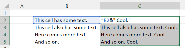
Concatenate the two text parts with the & sign.

In this example, you have existing in cells B2 to B5. You want to add the word “Cool.” to it. So, the formula in cell C2 is:

 =B2&" Cool."

Please note that I have added a space before the word cool (on purpose…). The reason is that between the previous full stops and the word cool should have a space.

You can now copy the new cell (range C2 to C5). Paste it using paste special on top of the existing cells as values if you want to fully replace the original text cells.

Method 3: Try a workaround to insert text with the Find & Replace function

Admittedly, this method is a little bit trial and error. If it works depends on your existing cells. The main idea is to replace text from the original cells with new text.

Let’s go back to our original example. You again want to add the word “Cool.” to your existing cells:

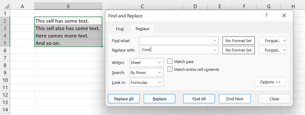
Insert text with the Find and Replace function.

In this case, we are lucky that all existing cells end with a full stop. We can use this to replace it the following way:

Select all original cells.
Press Ctrl + H on the keyboard so that the Find and Replace window opens.
As “Find what:”, enter “.”
Because we still want to keep the full stop, we also use this in the “Replace with:” field: “. Cool.”
Click on Replace All.

If the result is not as expected, you can simply undo the replace process (press Ctrl + Z on the keyboard).

Method 4: Bulk insert text with a VBA macro

If you feel comfortable to use a short VBA macro, you can copy and paste the following code into a new VBA module. Please refer to this article for help.

Replace the word ” Cool.” with your text to add at the end. Also, you can set a text to insert in the beginning. Then, place the cursor within these lines of code and press F5 on the keyboard.

Sub bulkInsertText()
    Dim textToInsertAtTheEnd As String, textToInsertAtTheBeginning As String
    
    'Replace "Cool" with your text to insert at the end
    textToInsertAtTheEnd = " Cool."
    textToInsertAtTheBeginning = ""
    
    For Each cell In Selection
        If cell.HasFormula = False Then
            cell.Value = textToInsertAtTheBeginning & cell.Value & textToInsertAtTheEnd
        End If
    Next
    
End Sub

Image by Gerd Altmann from Pixabay

Henrik Schiffner is a freelance business consultant and software developer. He lives and works in Hamburg, Germany. Besides being an Excel enthusiast he loves photography and sports.

Источник

Assuming that you have a list of data in range B1:B5 that contain string values and you want to add one character “E” after the first character of string in Cells. You can refer to the following two methods.

Table of Contents

1. Insert Character or Text to Cells with a Formula
2. Insert Character or Text to Cells with VBA
3. Video: Insert Character or Text to Cells
4. Related Functions

1. Insert Character or Text to Cells with a Formula

To insert the character to cells in Excel, you can use a formula based on the LEFT function and the MID function. Like this:

=LEFT(B1,1) & "E" & MID(B1,2,299)

Type this formula into a blank cell, such as: Cell C1, and press Enter key. And then drag the AutoFill Handle down to other cells to apply this formula.

insert text to cells1

This formula will inert the character “E” after the first character of string in Cells. And if you want to insert the character or text string after the second or third or N position of the string in Cells, you just need to replace the number 1 in Left function and the number 2 in MID function as 2 and 3. Like below:

=LEFT(B1,2) & "E" & MID(B1,3,299)

insert text to cells2

You can also use an Excel VBA Macro to insert one character or text after the first position of the text string in Cells. Just do the following steps:

Step1: open your excel workbook and then click on “Visual Basic” command under DEVELOPER Tab, or just press “ALT+F11” shortcut.

Step2: then the “Visual Basic Editor” window will appear.

Step3: click “Insert” ->”Module” to create a new module.

Step4: paste the below VBA code into the code window. Then clicking “Save” button.

insert text to cells3

Sub AddCharToCells()
    Dim cel As Range
    Dim curR As Range
    Set curR = Application.Selection
    Set curR = Application.InputBox("select one Range that you want to insert one 
    character", "add character to cells", curR.Address, Type: = 8)
    For Each cel In curR
        cel.Value = VBA.Left(cel.Value, 1) & "E" & VBA.Mid(cel.Value, 2, 
        VBA.Len(cel.Value) - 1)
    Next
End Sub

Step5: back to the current worksheet, then run the above excel macro. Click Run button.

insert text to cells4

Step6: select one Range that you want to insert one character.
insert text to cells5

Step7: lets see the result.

insert text to cells6

3. Video: Insert Character or Text to Cells

This video will demonstrate how to insert character or text in middle of cells in Excel using both formulas and VBA code.

Excel MID function
The Excel MID function returns a substring from a text string at the position that you specify.The syntax of the MID function is as below:= MID (text, start_num, num_chars)…
Excel LEFT function
The Excel LEFT function returns a substring (a specified number of the characters) from a text string, starting from the leftmost character.The LEFT function is a build-in function in Microsoft Excel and it is categorized as a Text Function.The syntax of the LEFT function is as below:= LEFT(text,[num_chars])…

Источник

In a scenario where you have a data table set up in a Word document, you can convert the table into an Excel sheet, by simply importing it – no need to recreate the table in Excel!

Likewise, you can also easily import a text Word document into Excel.

Import Word document into Excel as an embedded object.
Import Word data into multiple cells in Excel.
Import Word data as a text file into Excel.

We will show you in simple step-by-step instructions how you can do this.

Let us start.

Method #1: Import Word Document as an embedded object into Excel

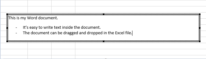
This is useful to create a central access point to various Word documents. By embedding the document into Excel, the Word document itself will open when you double click on it.

Step #1: Open an Excel spreadsheet

Open an Excel spreadsheet into which you want to import the Word data.

Step #2: Navigate to a cell

Navigate to the cell where you want to import the data.

Step #3: Import the data

Click on the ‘Insert’ tab in the top menu bar to change the ribbon.

In the section ‘Text’, click on Object.

This opens the ‘Insert Object’ dialog box.

Click on the option ‘Create from file’.

Ensure the options ‘Link to file’ and ‘Display as icon’ boxes are not ticked.

Click on the Browse… button.

This will open the File Manager/Explorer window.

Navigate to the Word document that you want to import.

Once you have selected it, click on the Insert button.

The name of the Word document will now appear in the ‘Insert Object’ dialog box.

Click on the OK button at the bottom.

Excel embeds the Word document as an object.

Method #2: Import Word Data into Multiple Cells in Excel

Step #1: Open a Word document

Open the Word document that contains the data you want to import.

Click on the cross symbol in the top left corner of the table to select it.

Press CTRL+C on the keyboard to copy the data into the clipboard, OR click right and select ‘Copy’ from the menu that opened.

Step #2: Close the Word document

Close the Word document. (Optional)

Step #3: Open the Excel spreadsheet

Open the Excel spreadsheet into which you want to import the Word data.

Step #4: Navigate to a cell

Navigate to the cell from where you want to start importing the data. The cell you select will be the upper left starting point of the data you want to import.

Step #5: Import the data

Right-click on this cell to open a menu.

Excel offers you two Paste Options:

Keep Source Formatting (K) — Paste the data as it appeared in Word (lines, font, and text size will remain the same as it was originally)
Match Destination Formatting (M) — Paste the data as it should appear in Excel (the font, text size, etc. will become the same as the rest of the spreadsheet)

Pick one of the choices to import the data.

Excel imports the data into multiple cells. In our example below, we chose Match Destination Formatting.

Method #3: Import Word Data as a Text File into Excel

This is useful if you have a simple Word document that only contains text – no images or graphs or tables.

If you have already created a project capturing information, but realize a spreadsheet will work better than a document, then this tool is for you to ensure you don’t have to redo your hard work.

Step #1: Open a Word document

Open the Word document that contains the data you want to import.

Click on the ‘File’ tab in the top menu bar.

This opens the ‘File’ menu.

In the left pane, click on the ‘Export’ option.

In the pane that opens, under Export, click on ‘Change File Type.’

Under the ‘Change File Type’ menu, select Plain Text.

Click on Save As.

Step #2: Save as a plain text document

This opens the File Manager.

Save your file as plain text type with an appropriate name. In some instances you will now see it saved as document_name.txt

Step #3: Close the Word document

Close the Word document. (Optional)

Step #4: Open the Excel spreadsheet

Open the Excel spreadsheet where you want to import the data.

Click on the ‘Data’ tab in the top menu bar to change the ribbon.

Step #5: Import the data

In the section ‘Get External Data’, click on the ‘From Text’ icon.

This opens the File Manager.

Navigate to the plain text file you have saved in step #2.

Click on the name of the plain text file.

Click on the Open button.

This opens the first dialog box of the Text Import Wizard.

Under the option ‘Choose the file type…’, click and select Delimited.

Make other changes if necessary.

Click on Next at the bottom of the dialog box.

This will open the second dialog box.

Click and select the ‘Tab’ option under ‘Delimiters’.

Make other changes if necessary.

Click on Next at the bottom of the dialog box.

This will open the third dialog box.

Under ‘Column data’ format, click and select ‘General’.

Make other changes if necessary.

Click on the Finish button at the bottom of the dialog box.

This opens the ‘Import Data’ dialog box.

Select the worksheet and the cell where Excel will import the data.

Click the OK button.

Excel imports the text data.

Step #6: Format the data

Right-click on the cell containing the data.

A menu opens.

Select ‘Format Cells…’

This opens the ‘Format Cells’ dialog box.

Click on the ‘Alignment’ tab.

Under ‘Text control’, click and select ‘Wrap Text’.

Make other changes if necessary.

Click on OK at the bottom of the dialog box.

Excel formats the text data to fit into one cell.

Conclusion

We have shown you three methods of inserting Word data into Excel, depending on your needs and the type of data in your Word document.

Источник

The good thing is you don’t need to do this manually.

Excel provides some really simple ways in which you can add text to the beginning and/ or end of the text in a range of cells.

In this tutorial we will see 4 ways to do this:

Using the ampersand operator (&)
Using the CONCATENATE function
Using the Flash Fill feature
Using VBA

So let’s get started!

Method 1: Using the ampersand Operator

An ampersand (&) can be used to easily combine text strings in Excel. Let’s see how you use it to add text at the beginning or end or both in Excel.

Using the ampersand Operator to Add Text to the Beginning of all Cells

The ampersand (&) is an operator that is mainly used to join several text strings into one.

Here’s how you can use it to add text to the beginning of all cells in a range. Let us assume you have the following list of names and want to add the title “Prof.” before every name:

Below are the steps to add a text before a text string in Excel:

Click on the first cell of the column where you want the converted names to appear (B2).
Type equal sign (=), followed by the text “Prof. “, followed by an ampersand (&).
Select the cell containing the first name (A2).
Press the Return Key.
You will notice that the title “Prof.” is added before the first name in the list.
It’s now time to copy this formula to the rest of the cells in the column. Simply double click the fill handle (located at the bottom right of cell B2). Alternatively, you can drag down the fill handle to achieve the same effect.

That’s it, all your cells in column B should now contain the title “Prof.” preceding each name.

Using the ampersand Operator to Add Text to the End of all Cells

Click on the first cell of the column where you want the converted names to appear (C2 in our case).
Type equal sign (=)
Select the cell containing the first name (B2 in our case).
Next, insert an ampersand (&), followed by the text “ (MD)”.
Press the Return Key.
You will notice that the text “(MD).” added after the first name in the list.
It’s now time to copy this formula to the rest of the cells in the column. Simply double click the fill handle (located at the bottom right of cell C2). Alternatively, you can drag down the fill handle to achieve the same effect.

All your cells in column C should now contain the text “(MD”) at the end of each name.

Adding text before and after a text string

Method 2: Using the CONCATENATE Function

CONCATENATE is an Excel function that you can use to add text at the beginning and end of the text string.

Let’s see how to use CONCATENATE to do this.

Using CONCATENATE to Add Text to the Beginning of all Cells

The CONCATENATE() function provides the same functionality as the ampersand (&) operator. The only difference is in the way both are used.

The general syntax for the CONCATENATE function is:

=CONCATENATE(text1, [text2], …)

Where text1, text2, etc. are substrings that you want to combine together.

Let’s apply the CONCATENATE function to the same dataset as above:

Click on the first cell of the column where you want the converted names to appear (B2).
Type equal sign (=).
Enter the function CONCATENATE, followed by an opening bracket (.
Type the title “Prof. ” in double-quotes, followed by a comma (,).
Select the cell containing the first name (A2)
Place a closing bracket. In our example, your formula should now be: =CONCATENATE(“Prof. “,A2).
Press the Return Key.
You will notice that the title “Prof.” is added before the first name on the list.
It’s now time to copy this formula to the rest of the cells in the column. Simply double click the fill handle (located at the bottom right of cell B2). Alternatively, you can drag down the fill handle to achieve the same effect.

That’s it, all your cells in column B should now contain the title “Prof.” preceding each name.

Using CONCATENATE to Add Text to the End of all Cells

Click on the first cell of the column where you want the converted names to appear (C2 in our example).
Type equal sign (=).
Enter the function CONCATENATE, followed by an opening bracket (.
Select the cell containing the first name (B2 in our example).
Next, insert a comma, followed by the text “ (MD)”.
Place a closing bracket. In our example, your formula should now be: =CONCATENATE(B2,” (MD)”).
Press the Return Key.
You will notice that the text “(MD).” added after the first name in the list.
It’s now time to copy this formula to the rest of the cells in the column. Simply double click the fill handle (located at the bottom right of cell C2).

All your cells in column C should now contain the text “(MD”) at the end of each name.

Notice that since you’re using a formula, your column C depends on columns A and B. So if you make any changes to the original values in column A, they get reflected in column C.

If you decide to only retain the converted names and delete columns A and B, you will get an error, as shown below:

Issue when deleting rhe dependent columns

Now you can go ahead and delete columns A and B if you need to.

Also read: How to Remove First Character in Excel?

Method 3: Using the Flash Fill Feature

Flash fill is a relatively new feature that looks at the pattern of what you are trying to achieve and then does it for all the cells in a column.

You can also use Flash fill to so text manipulation as we will see in the following examples.

Using Flash Fill to Add Text to the Beginning of all Cells

The Excel flash fill feature is like a magical button. It is available if you’re on any Excel version from 2013 onwards.

Here’s how you can use Flash Fill to add text to the beginning of all cells in a column:

Click on the first cell of the column where you want the converted names to appear (B2).
Manually type in the text Prof. , followed by the first name of your list.
Press the Return Key.
Click on cell B2 again.
Under the Data tab, click on the Flash Fill button (in the ‘Data Tools’ group). Alternatively, you can just press CTRL+E on your keyboard (Command+E if you’re on a Mac).

This will copy the same pattern to the rest of the cells in the column… in a flash!

Using Flash Fill to Add Text to the End of all Cells in a Column

If you want to add the text “ (MD)” to the end of the names, follow the same steps:

Click on the first cell of the column where you want the converted names to appear (C2).
Manually type in or copy the text from column B2 into C2.
Add the text “(MD)” after that.
Under the Data tab, click on the Flash Fill or press CTRL+E on your keyboard (Command+E if you’re on a Mac).

That’s all, you get every cell filled in with the same pattern!

We especially like this method because it is simple, quick, and easy. Moreover, since it’s formula-free, the results do not depend on the original columns.

So they remain unchanged even if you delete rows A and B!

Result in case you delete all the other columns

Method 4: Using VBA Code

And of course, if you’re comfortable with VBA, you can also add text before or after a text string using it.

Using VBA to Add Text to the Beginning of all Cells in a Column

If coding with VBA does not intimidate you then this method can help get your work done quickly too.

Here’s the code we will be using to add the title “Prof. “ to the beginning of all cells in a range. You can select and copy it:

Sub add_text_to_beginning()
Dim rng As Range
Dim cell As Range
Set rng = Application.Selection
For Each cell In rng
cell.Offset(0, 1).Value = "Prof. " & cell.Value
Next cell
End Sub

Follow these steps to use the above code:

From the Developer Menu Ribbon, select Visual Basic.
Once your VBA window opens, Click Insert->Module. Now you can start coding. Type or copy-paste the above lines of code into the module window. Your code is now ready to run.
Select the range of cells containing the text you want to convert. Make sure the column next to it is blank because this is where the code will display the results.
Navigate to Developer->Macros-> add_text_to_beginning->Run.

You will now see the converted text next to your selected range of cells.

Note: You can change the text in line 6 from “Prof. ” to whatever text you need to add to the beginning of all cells.

Using VBA to Add Text to the End of all Cells in a Column

cell.Offset(0, 1).Value = cell.Value & “ (MD)”

So your full code should now be:

Sub add_text_to_end()
Dim rng As Range
Dim cell As Range
Set rng = Application.Selection
For Each cell In rng
cell.Offset(0, 1).Value = cell.Value & " (MD)"
Next cell
End Sub

Here’s the final result:

You can now delete the first two columns if you need to. Do remember to keep a backup of your sheet, because the results of VBA code are usually irreversible.

Note: You can change the text in line 6 from “ (MD)” to whatever text you need to add to the end of all cells in the range.

In this tutorial, we showed you four ways in which you can add text to the beginning and/ or end of all cells in a range.

There are plenty of other methods that you can find online too, and all of them work just as well as the ones shown here.

You may feel free to choose whatever method suits you, your requirement, and your version of Excel. In the end, what matters is getting what you need to be done quickly and effectively.

Other Excel tutorials you may like:

How to Remove Text after a Specific Character in Excel
How to Reverse a Text String in Excel
How to Count How Many Times a Word Appears in Excel
How to Remove Commas in Excel (from Numbers or Text String)
How to Remove a Specific Character from a String in Excel
How to Change Uppercase to Lowercase in Excel
How to Separate Address in Excel?
How to Concatenate with Line Breaks in Excel?
How to Separate Names in Excel

Источник

Excel is a great tool for doing all the analysis and finalizing the report. But sometimes, calculation alone cannot convey the message to the reader because every reader has their way of looking at the report. Some people can understand the numbers just by looking at them, some need some time to get the real story, and some cannot understand. So, they need a full and clear-cut explanation of everything.

You can download this Text in Excel Formula Template here – Text in Excel Formula Template

To bring all the users to the same page while reading the report, we can add text comments to the formula to make the report easily readable.

Let us look at how we can add text in Excel formulas.

Formula with Text in Excel
- #1 – Add Meaningful Words Using with Text in Excel Formula
- #2 – Add Meaningful Words to Formula Calculations with TIME Format
- #3 – Add Meaningful Words to Formula Calculations with Date Format
- Things to Remember Formula with Text in Excel
- Recommended Articles

#1 – Add Meaningful Words Using Text in Excel Formula

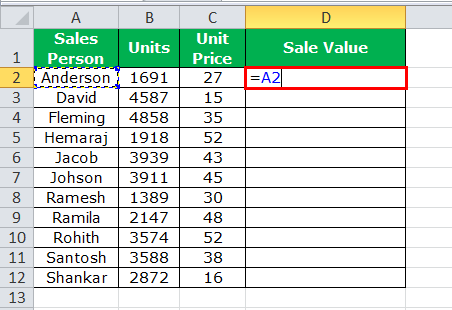
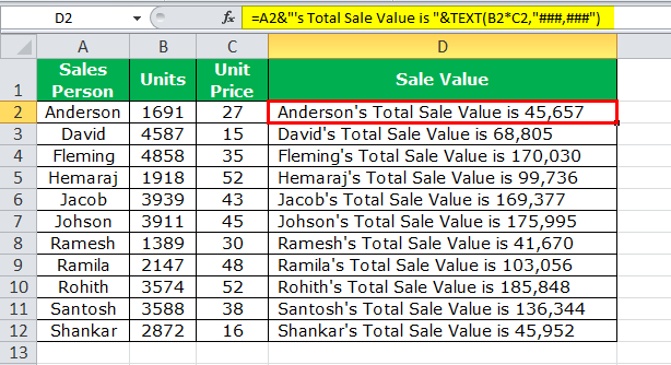
Often in Excel, we only perform calculations. Therefore, we are not worried about how well they convey the message to the reader. For example, take a look at the below data.

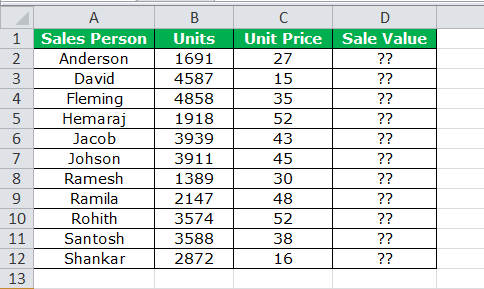
By looking at the above image, it is very clear that we need to find the sale value by multiplying Units to Unit PriceUnit Price is a measurement used for indicating the price of particular goods or services to be exchanged with customers or consumers for money. It includes fixed costs, variable costs, overheads, direct labour, and a profit margin for the organization.read more.

Apply simple text in the Excel formula to get the total sales value for each salesperson.

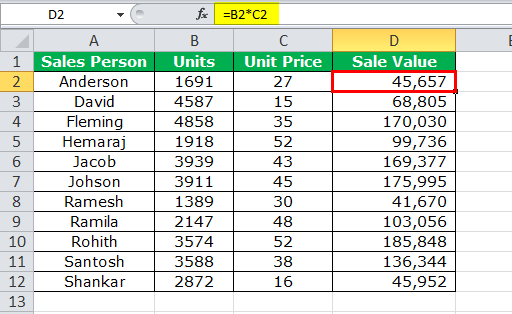
Usually, we stop the process here itself.

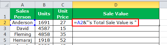
How about showing the calculation as Anderson’s total “Sale Value” is 45,657?

It looks like a complete sentence to convey a clear message to the user. So, let us go ahead and frame a sentence along with the formula.

So, let us go ahead and frame a sentence along with the formula.

We know the format of the sentence to be framed. Firstly, we need a “Sales Person” name to appear. So, we must select the cell A2 cell.
Now, we need “Total Sale Value” after the salesperson’s name. We need to put the ampersand operator sign after selecting the first cell to comb this text value.
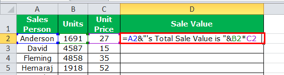
Now, we need to do the calculation to get the sale value. Put on more (ampersand) sign and apply the formula as B*C2.
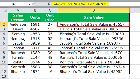
Now, we must press the “Enter” key to complete the formula and our text values.

One problem with this formula is that sales numbers are not formatted properly. Because they do not have a thousand separators, that would have made the numbers look properly.

There is nothing to worry about; we can format the numbers with the TEXT function in the Excel formula.

Edit the formula. As shown below, the calculation part applies the Excel TEXT function to format the numbers.

Now, we have the proper format of numbers along with the sales values. The TEXT function in Excel formula format the calculation (B2*C2) to the format of ###, ###.

#2 – Add Meaningful Words to Formula Calculations with TIME Format

We have seen how to add text values to our formulas to convey a clear-cut message to the readers or users. Now, we will be adding text values to another calculation, which includes time calculations.

We have data on flight departure and arrival timings. We need to calculate the total duration of each flight.

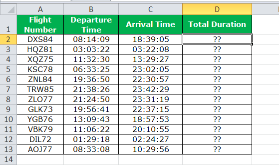
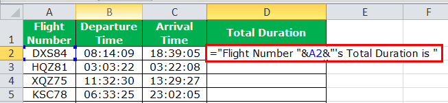
Not only the total duration, but we want to show the message like this “Flight Number DXS84’s total duration is 10:24:56.”

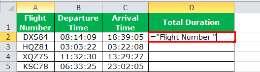
In cell D2, we must start the formula. Our first value is “Flight Number.” We must enter this in double-quotes.

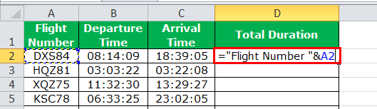
The next value we need to add is the flight number already in cell A2. Enter the “&” symbol and select cell A2.

The next thing we need to add to the text‘s “Total Duration.”We must insert one more “&”symbol and enter this text in double-quotes.

Now comes the most important part of the formula. We need to calculate the total duration after “&” the symbol enters the formula as C2 – B2.

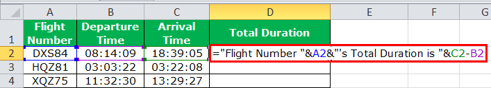
Our full calculation is complete. Press the “Enter” key to get the result.

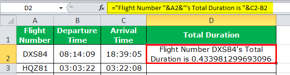
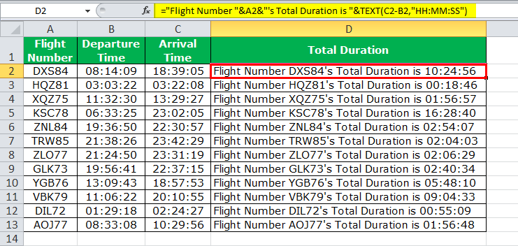
We got the total duration as 0.433398, which is not in the right format. So, we must apply the TEXT function to perform the calculation and format that to TIME.

#3 – Add Meaningful Words to Formula Calculations with Date Format

The TEXT function can perform the formatting task when adding text values to get the correct number format. Now, we will see it in the date format.

Below is the daily sales table that we update the values regularly.

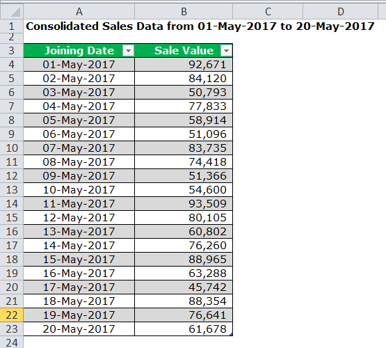
We need to automate the heading as the data keeps adding, i.e., we should change the last date as per the last day of the table.

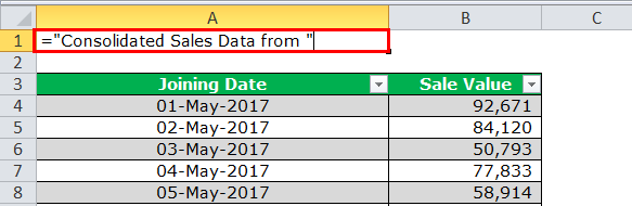
Step 1: We must first open the formula in the A1 cell as “Consolidated Sales Data from.”

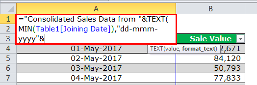
Step 2: Put the “&” symbol and apply the TEXT function in the Excel formula. Apply the MIN function to get the least date from this list inside the TEXT function. And format it as “dd-mmm-yyyy.”

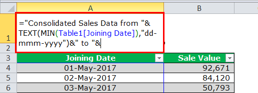
Step 3: Now, enter the word to.

Step 4: To get the latest date from the table, we must apply the MAX formulaThe MAX Formula in Excel is used to calculate the maximum value from a set of data/array. It counts numbers but ignores empty cells, text, the logical values TRUE and FALSE, and text values.read more, and format it as the date by using TEXT in the Excel formula.

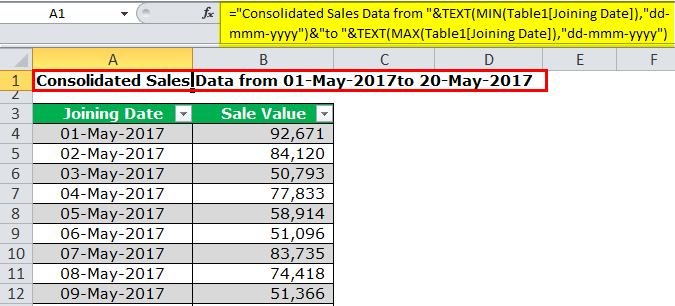
As we update the table, it will automatically update the heading.

Things to Remember Formula with Text in Excel

We can add the text values according to our preferences by using the CONCATENATE function in excelThe CONCATENATE function in Excel helps the user concatenate or join two or more cell values which may be in the form of characters, strings or numbers.read more or the ampersand (&) symbol.
To get the correct number format, we must use the TEXT function and specify the number format we want to display.

Insert an object in your Excel spreadsheet

Insert Character or Text to Cells

Insert Character or Text to Cells with a Formula

Insert Character or Text to Cells with VBA

Insert an object in your Excel spreadsheet

How to Add Text to the Beginning or End of all Cells in Excel

Method 1: Using the ampersand Operator

Using the ampersand Operator to Add Text to the Beginning of all Cells

Using the ampersand Operator to Add Text to the End of all Cells

Method 2: Using the CONCATENATE Function

Using CONCATENATE to Add Text to the Beginning of all Cells

Using CONCATENATE to Add Text to the End of all Cells

Method 3: Using the Flash Fill Feature

Using Flash Fill to Add Text to the Beginning of all Cells

Using Flash Fill to Add Text to the End of all Cells in a Column

Method 4: Using VBA Code

Using VBA to Add Text to the Beginning of all Cells in a Column

Using VBA to Add Text to the End of all Cells in a Column

Embed an object in a worksheet

Insert a link to a file

Create a new object from inside Excel

Embed an object in a worksheet

Insert a link to a file

Create a new object from inside Excel

Link or embed content from another program by using OLE

Change the way that an OLE object is displayed

Control updates to linked objects

Set a link to another program to be updated manually

Set a link to another program to be updated automatically

Update a link to another program now

Edit content from an OLE program

Select an OLE object by using the keyboard

Issue: When I double-click a linked or embedded object, a «cannot edit» message appears

Need more help?

Method 1: The fastest way to bulk insert text

Method 2: Use a string formula to combine two text parts

Method 3: Try a workaround to insert text with the Find & Replace function

Method 4: Bulk insert text with a VBA macro

1. Insert Character or Text to Cells with a Formula

3. Video: Insert Character or Text to Cells

Method #1: Import Word Document as an embedded object into Excel

Step #1: Open an Excel spreadsheet

Step #2: Navigate to a cell

Step #3: Import the data

Method #2: Import Word Data into Multiple Cells in Excel

Step #1: Open a Word document

Step #2: Close the Word document

Step #3: Open the Excel spreadsheet

Step #4: Navigate to a cell

Step #5: Import the data

Method #3: Import Word Data as a Text File into Excel

Step #1: Open a Word document

Step #2: Save as a plain text document

Step #3: Close the Word document

Step #4: Open the Excel spreadsheet

Step #5: Import the data

Step #6: Format the data

Conclusion

Method 1: Using the ampersand Operator

Using the ampersand Operator to Add Text to the Beginning of all Cells

Using the ampersand Operator to Add Text to the End of all Cells

Method 2: Using the CONCATENATE Function

Using CONCATENATE to Add Text to the Beginning of all Cells

Using CONCATENATE to Add Text to the End of all Cells

Method 3: Using the Flash Fill Feature

Using Flash Fill to Add Text to the Beginning of all Cells

Using Flash Fill to Add Text to the End of all Cells in a Column

Method 4: Using VBA Code

Using VBA to Add Text to the Beginning of all Cells in a Column

Using VBA to Add Text to the End of all Cells in a Column

Table of contents

#1 – Add Meaningful Words Using Text in Excel Formula

#2 – Add Meaningful Words to Formula Calculations with TIME Format

#3 – Add Meaningful Words to Formula Calculations with Date Format

Things to Remember Formula with Text in Excel

Recommended Articles