Insert row after excel - Word и Excel - помощь в работе с программами

Insert or delete rows and columns

Insert and delete rows and columns to organize your worksheet better.

Note: Microsoft Excel has the following column and row limits: 16,384 columns wide by 1,048,576 rows tall.

Insert or delete a column

Select any cell within the column, then go to Home > Insert > Insert Sheet Columns or Delete Sheet Columns.
Alternatively, right-click the top of the column, and then select Insert or Delete.

Insert or delete a row

Select any cell within the row, then go to Home > Insert > Insert Sheet Rows or Delete Sheet Rows.
Alternatively, right-click the row number, and then select Insert or Delete.

Formatting options

When you select a row or column that has formatting applied, that formatting will be transferred to a new row or column that you insert. If you don’t want the formatting to be applied, you can select the Insert Options button after you insert, and choose from one of the options as follows:

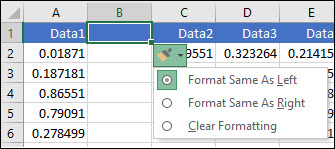
If the Insert Options button isn’t visible, then go to File > Options > Advanced > in the Cut, copy and paste group, check the Show Insert Options buttons option.

Insert rows

To insert a single row: Right-click the whole row above which you want to insert the new row, and then select Insert Rows.

To insert multiple rows: Select the same number of rows above which you want to add new ones. Right-click the selection, and then select Insert Rows.

Insert columns

To insert a single column: Right-click the whole column to the right of where you want to add the new column, and then select Insert Columns.

To insert multiple columns: Select the same number of columns to the right of where you want to add new ones. Right-click the selection, and then select Insert Columns.

Delete cells, rows, or columns

If you don’t need any of the existing cells, rows or columns, here’s how to delete them:

Select the cells, rows, or columns that you want to delete.
Right-click, and then select the appropriate delete option, for example, Delete Cells & Shift Up, Delete Cells & Shift Left, Delete Rows, or Delete Columns.

When you delete rows or columns, other rows or columns automatically shift up or to the left.

Tip: If you change your mind right after you deleted a cell, row, or column, just press Ctrl+Z to restore it.

Insert cells

To insert a single cell:

Right-click the cell above which you want to insert a new cell.
Select Insert, and then select Cells & Shift Down.

To insert multiple cells:

Select the same number of cells above which you want to add the new ones.
Right-click the selection, and then select Insert > Cells & Shift Down.

Need more help?

You can always ask an expert in the Excel Tech Community or get support in the Answers community.

CURRENT TABLE:

column1   |   column2   |  column3
----------------------------------
  A       |     small   |  blue
  A       |     small   |  orange
  A       |     small   |  yellow
  B       |     med     |  yellow
  B       |     med     |  blue
  C       |     large   |  green
  D       |     large   |  green
  D       |     small   |  pink

DESIRED TABLE

Note: the blank row after each distinct column1

column1   |   column2   |  column3
----------------------------------
  A       |     small   |  blue
  A       |     small   |  orange
  A       |     small   |  yellow

  B       |     med     |  yellow
  B       |     med     |  blue

  C       |     large   |  green

  D       |     large   |  green
  D       |     small   |  pink

asked Mar 14, 2013 at 18:39

This does exactly what you are asking, checks the rows, and inserts a blank empty row at each change in column A:

sub AddBlankRows()
'
dim iRow as integer, iCol as integer
dim oRng as range

set oRng=range("a1")

irow=oRng.row
icol=oRng.column

do 
'
if cells(irow+1, iCol)<>cells(irow,iCol) then
    cells(irow+1,iCol).entirerow.insert shift:=xldown
    irow=irow+2
else
    irow=irow+1
end if
'
loop while not cells (irow,iCol).text=""
'
end sub

I hope that gets you started, let us know!

Philip

answered Mar 14, 2013 at 19:15

Select your array, including column labels, DATA > Outline -Subtotal, At each change in: column1, Use function: Count, Add subtotal to: column3, check Replace current subtotals and Summary below data, OK.

Filter and select for Column1, Text Filters, Contains…, Count, OK. Select all visible apart from the labels and delete contents. Remove filter and, if desired, ungroup rows.

answered Oct 20, 2015 at 6:08

pnutspnuts

58k11 gold badges85 silver badges137 bronze badges

This won’t work if the data is not sequential (1 2 3 4 but 5 7 3 1 5) as in that case you can’t sort it.

Here is how I solve that issue for me:

Column A initial data that needs to contain 5 rows between each number —
5
4
6
8
9

Column B —
1
2
3
4
5
(final number represents the number of empty rows that you need to be between numbers in column A) copy-paste 1-5 in column B as long as you have numbers in column A.

Jump to D column, in D1 type 1. In D2 type this formula — =IF(B2=1,1+D1,D1)
Drag it to the same length as column B.

Back to Column C — at C1 cell type this formula — =IF(B1=1,INDIRECT("a"&(D1)),""). Drag it down and we done. Now in column C we have same sequence of numbers as in column A distributed separately by 4 rows.

answered May 1, 2016 at 13:21

Figured it out.

Step 1

Put a new column to the left of column1 and copy+paste the following formula

=B2=B3

=B3=B4

=B4=B5

… all the way to the bottom (assume column B here is column1 in the original question).

This formula evaluates whether or not the next row is a new value in column1. Deopending on the result, you will have TRUE or FALSE. Copy and Paste these results as values and then swap «FALSE» for nil and «TRUE» for 0.5

Step 2

Then add that column full of only 0.5’s to the column1 which will yield the following table:

  newcolumn0  |   column1 ("B") |   column2   |  column3
-----------------------------------------------------
              |     1           |     small   |  blue
              |     1           |     small   |  orange
      1.5     |     1           |     small   |  yellow
              |     2           |     med     |  yellow
      2.5     |     2           |     med     |  blue
      3.5     |     3           |     large   |  green
              |     4           |     large   |  green
      4.5     |     4           |     small   |  pink

Step 3

Lastly, copy and paste the values from newcolumn0 right below the values in column1 and then sort the table by column1 and you should have a blank row in between each distinct whole number in column1, with the table something like this:

    newcolumn0   |  column1 ("B")  |   column2       |  column3
---------------------------------------------------------------
                 |     1           |     small   |  blue
                 |     1           |     small   |  orange
        1.5      |     1.5         |             |
                 |     1           |     small   |  yellow
                 |     2           |     med     |  yellow
                 |     2           |     med     |  blue
        2.5      |     2.5         |             |
                 |     3           |     large   |  green
        3.5      |     3.5         |             |
                 |     4           |     large   |  green
                 |     4           |     small   |  pink
        4.5      |     4.5         |             |

Alternative Solutions (still no VBA)

Put a value of 1 Column 1, Row 2 (assume this is A2)
Put this formula in A3 =IF(B3=B2,A2,A2+1) and copy+paste this formula for the rest of column 2
Then copy and paste all the values from column 1 into a new temp excel sheet, remove duplicates, then add 0.5 to all numbers, then paste these values below the values in original spreadsheet below the data in column 1, paste all data in column as values and then sort by that column, delete the temp excel sheet

answered Mar 14, 2013 at 19:13

BenBen

1,0134 gold badges16 silver badges34 bronze badges

Just an idea, if you know the categories, as small, medium, and large mentioned above…

At the bottom of the sheet, make 3 rows that only say small, medium, and large, change the font to white, and then sort so that it alphabetizes, placing a blank row between each section.

answered Jan 16, 2017 at 18:34

Insert a column at the left of the table ‘Control’
Number the data as 1 to 1000 (assuming there are 1000 rows)
Copy the key field to another sheet and remove duplicates
Copy the unique row items to the main sheet, after 1000th record
In the ‘Control’ column, add number 1001 to all unique records
Sort the data (including the added records), first on key field and then on ‘Control’
A blank line (with data in key field and ‘Control’) is added

answered Mar 29, 2017 at 7:17

I have a large file in excel dealing with purchase and sale of mutual fund units. Number of rows in a worksheet exceeds 4000. I have no experience with VBA and would like to work with basic excel. Taking the cue from the solutions suggested above, I tried to solve the problem ( to insert blank rows automatically) in the following manner:

I sorted my file according to control fields
I added a column to the file
I used the «IF» function to determine when there is a change in the control data .
If there is a change the result will indicate «yes», otherwise «no»
Then I filtered the data to group all «yes» items
I copied mutual fund names, folio number etc (no financial data)
Then I removed the filter and sorted the file again. The result is a row added at the desired place. (It is not entirely a blank row, because if it is fully blank, sorting will not place the row at the desired place.)
After sorting, you can easily delete all values to get a completely blank row.

This method also may be tried by the readers.

answered Nov 12, 2015 at 8:12

Источник

Hello, Excellers. Welcome back to another blog post in my #Excel 2021 series. Today let’s look at a really useful but very straightforward Excel tip. I will show you how to insert a blank row after every data row in your Excel worksheet. No formulas, not macros and no coding. Here a sample data set to work with below.

First a helper column is needed. So, if the data starts in Column A in the Excel worksheet insert a column to allow your data to start in Column B. Column A is going to be used for this helper column.

To start, type 1 in the first cell of your helper column. This should be in the first row of data. Avoid the header row. The next step is also easy highlight all cell in Column A to the bottom of your data set. My example is easy. It only contains 16 lines of data. Use the Excel shortcut Ctrl+Shift+Down Arrow to quickly highlight the full column of data if required.

Next, use the fill series to fil the row numbers.

Home Tab
Editing Group
Fill | Fill Series
Complete the Step value (1 in this example)
The stop value is the last rows of data (14 in this example)

Hit ok. Excel fills the series accordingly.

The final part of this tip is clever. Copy the Fill series from the steps above and past below the last row of data. This will be used to insert the blank row after each data row.

Finally, select the full data set.

On the Home Tab go to the Editing Group.
Sort and Filter.
Sort Smallest To Largest.
That is it job done. Each blank row is inserted.
Delete the helper column.

So, What Next? Want More Tips?

If you want more Excel and VBA tips then sign up to my Monthly Newsletter where I share 3 Tips on the first Wednesday of the month. You will receive my free Ebook, 30 Excel Tips. Why not check out all of my Macro Monday and Formula Friday blog posts below.

Macro Monday Blog Posts

Formula Friday Blog Posts.

Источник

Вставка диапазона со сдвигом ячеек вправо или вниз методом Insert объекта Range. Вставка и перемещение строк и столбцов из кода VBA Excel. Примеры.

Range.Insert – это метод, который вставляет диапазон пустых ячеек (в том числе одну ячейку) на рабочий лист Excel в указанное место, сдвигая существующие в этом месте ячейки вправо или вниз. Если в буфере обмена содержится объект Range, то вставлен будет он со своими значениями и форматами.

Синтаксис

Expression.Insert(Shift, CopyOrigin)

Expression – выражение (переменная), возвращающее объект Range.

Параметры

Параметр	Описание	Значения
Shift	Необязательный параметр. Определяет направление сдвига ячеек. Если параметр Shift опущен, направление выбирается в зависимости от формы* диапазона.	xlShiftDown (-4121) – ячейки сдвигаются вниз; xlShiftToRight (-4161) – ячейки сдвигаются вправо.
CopyOrigin	Необязательный параметр. Определяет: из каких ячеек копировать формат. По умолчанию формат копируется из ячеек сверху или слева.	xlFormatFromLeftOrAbove (0) – формат копируется из ячеек сверху или слева; xlFormatFromRightOrBelow (1) – формат копируется из ячеек снизу или справа.

* Если диапазон горизонтальный или квадратный (количество строк меньше или равно количеству столбцов), ячейки сдвигаются вниз. Если диапазон вертикальный (количество строк больше количества столбцов), ячейки сдвигаются вправо.

Примеры

Простая вставка диапазона

Вставка диапазона ячеек в диапазон «F5:K9» со сдвигом исходных ячеек вправо:

Range(«F5:K9»).Insert Shift:=xlShiftToRight

Если бы параметр Shift не был указан, сдвиг ячеек, по умолчанию, произошел бы вниз, так как диапазон горизонтальный.

Вставка вырезанного диапазона

Вставка диапазона, вырезанного в буфер обмена методом Range.Cut, из буфера обмена со сдвигом ячеек по умолчанию:

Range(«A1:B6»).Cut

Range(«D2»).Insert

Обратите внимание, что при использовании метода Range.Cut, точка вставки (в примере: Range("D2")) не может находится внутри вырезанного диапазона, а также в строке или столбце левой верхней ячейки вырезанного диапазона вне вырезанного диапазона (в примере: строка 1 и столбец «A»).

Вставка скопированного диапазона

Вставка диапазона, скопированного в буфер обмена методом Range.Copy, из буфера обмена со сдвигом ячеек по умолчанию:

Range(«B2:D10»).Copy

Range(«F2»).Insert

Обратите внимание, что при использовании метода Range.Copy, точка вставки (в примере: Range("F2")) не может находится внутри скопированного диапазона, но в строке или столбце левой верхней ячейки скопированного диапазона вне скопированного диапазона находится может.

Вставка и перемещение строк

Вставка одной строки на место пятой строки со сдвигом исходной строки вниз:

Вставка четырех строк на место пятой-восьмой строк со сдвигом исходных строк вниз:

Вставка строк с использованием переменных, указывающих над какой строкой осуществить вставку и количество вставляемых строк:

Sub Primer1()

Dim n As Long, k As Long, s As String

‘Номер строки, над которой необходимо вставить строки

n = 8

‘Количесто вставляемых строк

k = 4

‘Указываем адрес диапазона строк

s = n & «:» & (n + k — 1)

‘Вставляем строки

Rows(s).Insert

End Sub

‘или то же самое с помощью цикла

Sub Primer2()

Dim n As Long, k As Long, i As Long

n = 8

k = 4

For i = 1 To k

Rows(n).Insert

End Sub

Перемещение второй строки на место шестой строки:

Rows(2).Cut

Rows(6).Insert

Вторая строка окажется на месте пятой строки, так как третья строка заместит вырезанную вторую строку, четвертая встанет на место третьей и т.д.

Перемещение шестой строки на место второй строки:

Rows(6).Cut

Rows(2).Insert

В этом случае шестая строка окажется на месте второй строки.

Вставка и перемещение столбцов

Вставка одного столбца на место четвертого столбца со сдвигом исходного столбца вправо:

Вставка трех столбцов на место четвертого-шестого столбцов со сдвигом исходных столбцов вправо:

Перемещение третьего столбца на место седьмого столбца:

Columns(3).Cut

Columns(7).Insert

Третий столбец окажется на месте шестого столбца, так как четвертый столбец заместит вырезанный третий столбец, пятый встанет на место четвертого и т.д.

Перемещение седьмого столбца на место третьего столбца:

Columns(7).Cut

Columns(3).Insert

В этом случае седьмой столбец окажется на месте третьего столбца.

Источник

Creating new tables, reports and pricelists of different types, we cannot predict the number of necessary rows and columns. Using Excel program implies to a great extent creating and setting up spreadsheets, which requires inserting and deleting different elements.

First, let’s consider the methods of inserting sheet rows and columns when creating spreadsheets.

Note that in this tutorial we indicate hot keys for adding or deleting rows and columns. They should be used after highlighting the whole row or column. To highlight the row where the cursor is placed, press the combination of hot keys: SHIFT+SPACEBAR. Hot keys for highlighting a column are CTRL+SPACEBAR.

How to insert a column between other columns?

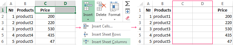
Assuming you have a pricelist lacking line item numbering:

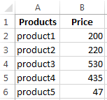
To insert a column between other columns for filling in pricelist items numbering you can use one of the two ways:

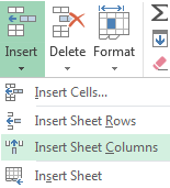
Move the cursor to activate A1 cell. Then go to tab «HOME», tool section «Cells» and click «Insert», in the popup menu select «Insert Sheet Columns» option.

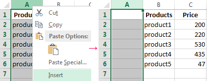
Right-click the heading of column A. Select «Insert» option on the shortcut menu.

Select the column, and press the hotkey combination CTRL+SHIFT+PLUS.

Now you can type the numbers of pricelist line items.

Simultaneous insertion of several columns

The pricelist still lacks two columns: quantity and units (items, kilograms, liters, packs). To add simultaneously, highlight the two-cell range (C1:D1). Then use the same tool on the «Insert»-«Insert Sheet Columns» main tab.

Alternatively, highlight two headings of columns C and D, right-click and select «Insert» option.

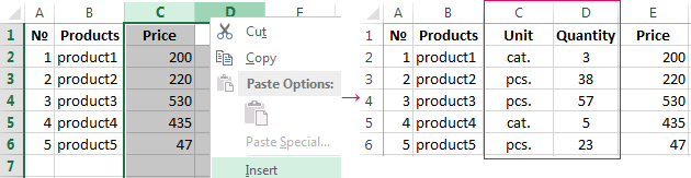
Note. Columns are always added to the left side. There appear as many new columns as many old ones have been highlighted. The order of inserted also depends on the order of highlighting. For example, next but one etc.

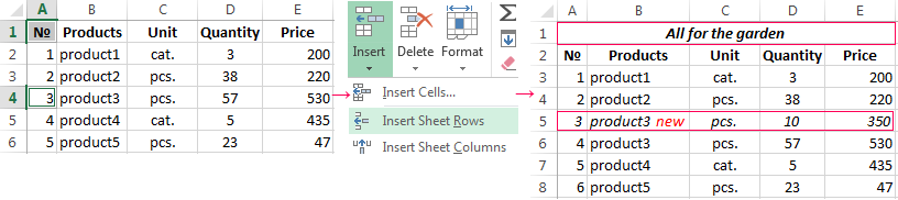
How to insert a row between rows in Excel?

Now let’s add a heading and a new goods line item «All for the garden» to the pricelist. To this end, let’s insert two new rows simultaneously.

Highlight the nonadjacent range of two cells A1,A4 (note that character “,” is used instead of character “:” – it means that two nonadjacent ranges should be highlighted; to make sure, type A1; A4 in the name field and press Enter). You know from the previous tutorials how to highlight nonadjacent ranges.

Now once again use the tool «HOME»-«Insert»-«Insert Sheet Columns». The picture shows how to insert a blank row between other rows in Excel.

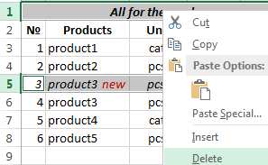
It is easy to guess the second way. You need to highlight headings of rows 1 and 3, right-click on one of the highlighted rows and select «Insert» option.

To add a row or a column in Excel use hot keys CTRL+SHIFT+PLUS having highlighted the appropriate row or column.

Note. New rows are always added above the highlighted rows.

Deleting rows and columns

When working with Excel you need to delete rows and columns as often as to insert them. Therefore, you have to practice.

By way of illustration, let’s delete from our pricelist the numbering of goods line items and the unit column simultaneously.

Highlight the nonadjacent range of cells A1; D1 and select «HOME»-«Delete»-«Delete Sheet Rows». The shortcut menu can also be used for deleting if you highlight headings A1 and D1 instead of cells.

Row deleting is performed in the similar way. You only need to select a tool in the appropriate menu. Applying a shortcut menu is the same. You only have to highlight the rows correspondingly by row numbers.

To delete a row or a column in Excel, use hot keys CTRL+MINUS having preliminary highlighted them.

Note. Inserting new columns and rows is in fact substitution, as the number of rows (1 048 576) and columns (16 384) doesn’t change. The new just replace the old ones. You should consider this fact when filling in the sheet with data by more than 50% — 80%.

Источник

Insert or delete a column

Insert or delete a row

Formatting options

Insert rows

Insert columns

Delete cells, rows, or columns

Insert cells

Need more help?

See Also

Need more help?

CURRENT TABLE:

DESIRED TABLE

Step 1

Step 2

Step 3

Alternative Solutions (still no VBA)

So, What Next? Want More Tips?

If you want more Excel and VBA tips then sign up to my Monthly Newsletter where I share 3 Tips on the first Wednesday of the month. You will receive my free Ebook, 30 Excel Tips. Why not check out all of my Macro Monday and Formula Friday blog posts below.

Macro Monday Blog Posts

Formula Friday Blog Posts.

Синтаксис

Параметры

Примеры

Простая вставка диапазона

Вставка вырезанного диапазона

Вставка скопированного диапазона

Вставка и перемещение строк

Вставка и перемещение столбцов

How to insert a column between other columns?

Simultaneous insertion of several columns

How to insert a row between rows in Excel?

Deleting rows and columns