
Watch Video – How to Insert Picture into a Cell in Excel
A few days ago, I was working with a data set that included a list of companies in Excel along with their logos.
I wanted to place the logo of each company in the cell adjacent to its name and lock it in such a way that when I resize the cell, the logo should resize as well.
I also wanted the logos to get filtered when I filter the name of the companies.
Wishful Thinking? Not Really.
You can easily insert a picture into a cell in Excel in a way that when you move, resize, and/or filter the cell, the picture also moves/resizes/filters.
Below is an example where the logos of some popular companies are inserted in the adjacent column, and when the cells are filtered, the logos also get filtered with the cells.
This could also be useful if you’re working with products/SKUs and their images.
When you insert an image in Excel, it not linked to the cells and would not move, filter, hide, and resize with cells.
In this tutorial, I will show you how to:
- Insert a Picture Into a Cell in Excel.
- Lock the Picture in the cell so that it moves, resizes, and filters with the cells.
Insert Picture into a Cell in Excel
Here are the steps to insert a picture into a cell in Excel:
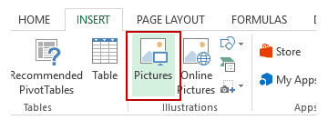
- Go to the Insert tab.
- Click on the Pictures option (it’s in the illustrations group).

- In the ‘Insert Picture’ dialog box, locate the pictures that you want to insert into a cell in Excel.

- Click on the Insert button.
- Re-size the picture/image so that it can fit perfectly within the cell.

- Place the picture in the cell.
- A cool way to do this is to first press the ALT key and then move the picture with the mouse. It will snap and arrange itself with the border of the cell as soon it comes close to it.

- A cool way to do this is to first press the ALT key and then move the picture with the mouse. It will snap and arrange itself with the border of the cell as soon it comes close to it.
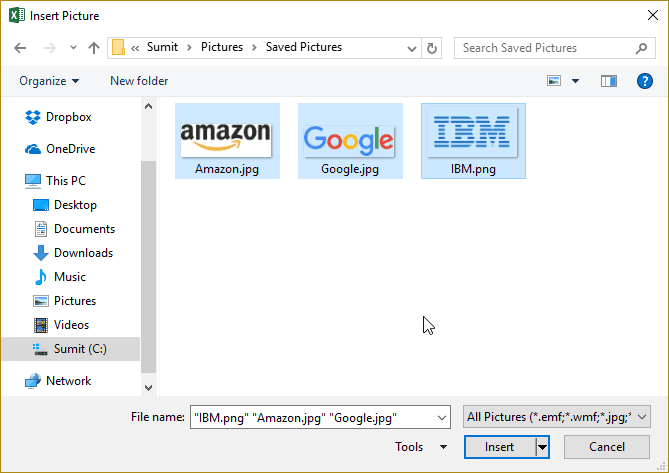


If you have multiple images, you can select and insert all the images at once (as shown in step 4).
You can also resize images by selecting it and dragging the edges. In the case of logos or product images, you may want to keep the aspect ratio of the image intact. To keep the aspect ratio intact, use the corners of an image to resize it.
When you place an image within a cell using the steps above, it will not stick with the cell in case you resize, filter, or hide the cells. If you want the image to stick to the cell, you need to lock the image to the cell it’s placed n.
To do this, you need to follow the additional steps as shown in the section below.
Lock the Picture with the Cell in Excel
Once you have inserted the image into the workbook, resized it ti fit within a cell, and placed it in the cell, you need to lock it to make sure it moves, filters, and hides with the cell.
Here are the steps to lock a picture in a cell:
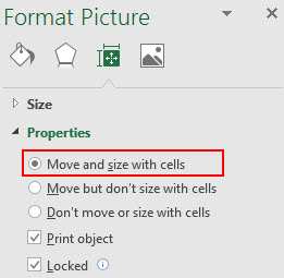
- Right-click on the picture and select Format Picture.

- In the Format Picture pane, select Size & Properties and with the options in Properties, select ‘Move and size with cells’.


That’s It!
Now you can move cells, filter it, or hide it, and the picture will also move/filter/hide.
Try it yourself.. Download the Example File

This could be a useful trick when you have a list of products with their images, and you want to filter certain categories of products along with their images.
You can also use this trick while creating Excel Dashboards.
You May Also Like the Following Excel Tutorials:
- Insert a Picture in a Comment in Excel.
- Insert Line Break in Excel Formula result.
- Picture Lookup Technique using Named Ranges.
- How to Insert Watermark in Excel Worksheets.
- How to Lock Cells in Excel.
Содержание
- Особенности вставки картинок
- Вставка изображения на лист
- Редактирование изображения
- Прикрепление картинки
- Способ 1: защита листа
- Способ 2: вставка изображения в примечание
- Способ 3: режим разработчика
- Вопросы и ответы

Некоторые задачи, выполняемые в таблицах, требуют установки в них различных изображений или фото. Программа Excel имеет инструменты, которые позволяют произвести подобную вставку. Давайте разберемся, как это сделать.
Особенности вставки картинок
Для того, чтобы вставить изображение в таблицу Эксель, оно сначала должно быть загружено на жесткий диск компьютера или подключенный к нему съёмный носитель. Очень важной особенностью вставки рисунка является то, что он по умолчанию не привязывается к конкретной ячейке, а просто размещается в выбранной области листа.
Урок: Как вставить картинку в Microsoft Word
Вставка изображения на лист
Сначала выясним, как вставить рисунок на лист, а уже потом разберемся, как прикрепить картинку к конкретной ячейке.
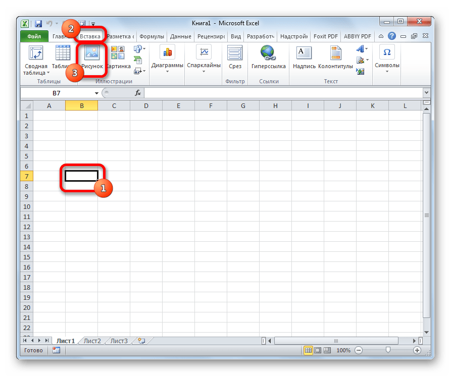
- Выделяем ту ячейку, куда вы хотите вставить изображение. Переходим во вкладку «Вставка». Кликаем по кнопке «Рисунок», которая размещена в блоке настроек «Иллюстрации».
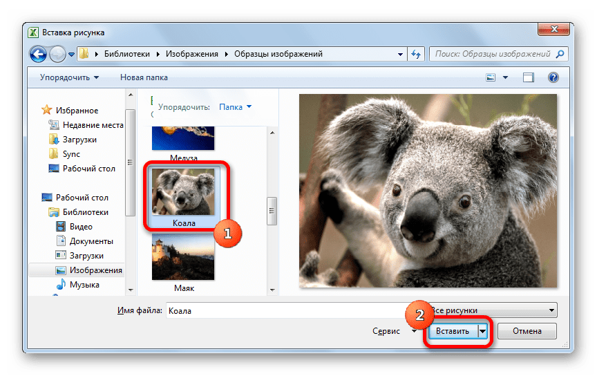
- Открывается окно вставки рисунка. По умолчанию оно всегда открывается в папке «Изображения». Поэтому вы можете предварительно перебросить в неё ту картинку, которую собираетесь вставить. А можно поступить другим путем: через интерфейс этого же окна перейти в любую другую директорию жесткого диска ПК или подключенного к нему носителя. После того, как вы произвели выбор картинки, которую собираетесь добавить в Эксель, жмите на кнопку «Вставить».
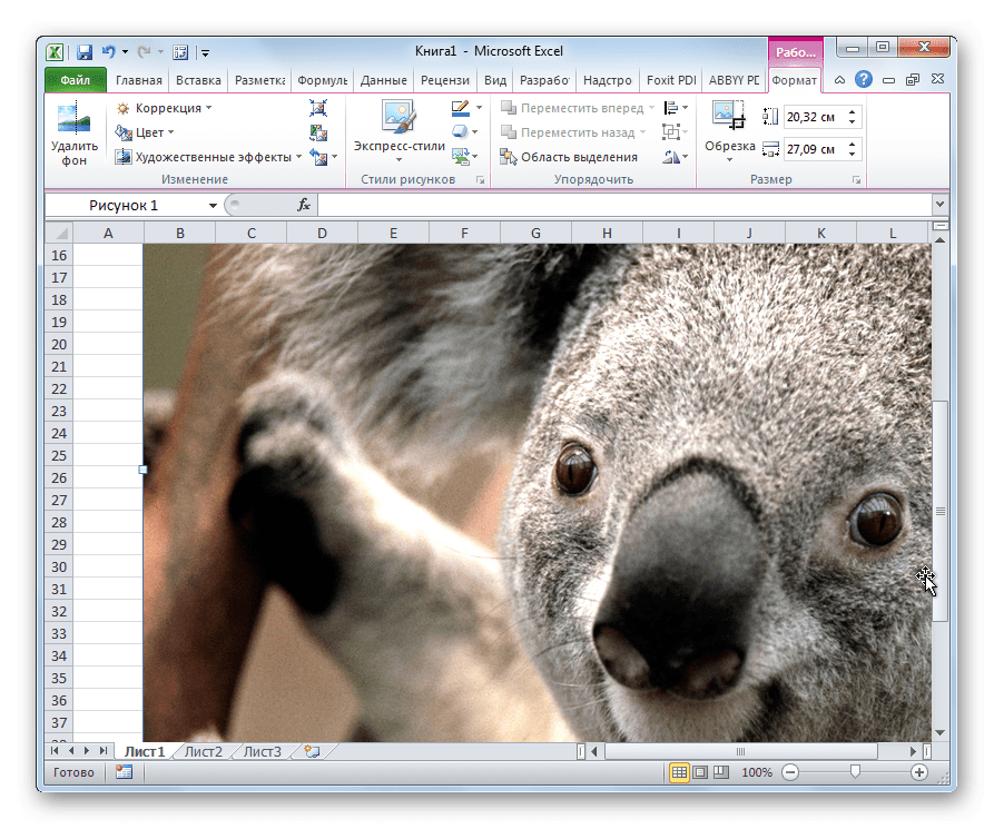
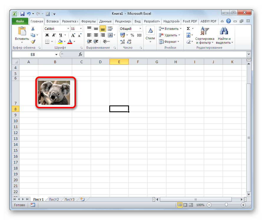
После этого рисунок вставляется на лист. Но, как и говорилось ранее, он просто лежит на листе и фактически ни с одной ячейкой не связан.
Редактирование изображения
Теперь нужно отредактировать картинку, придать ей соответствующие формы и размер.
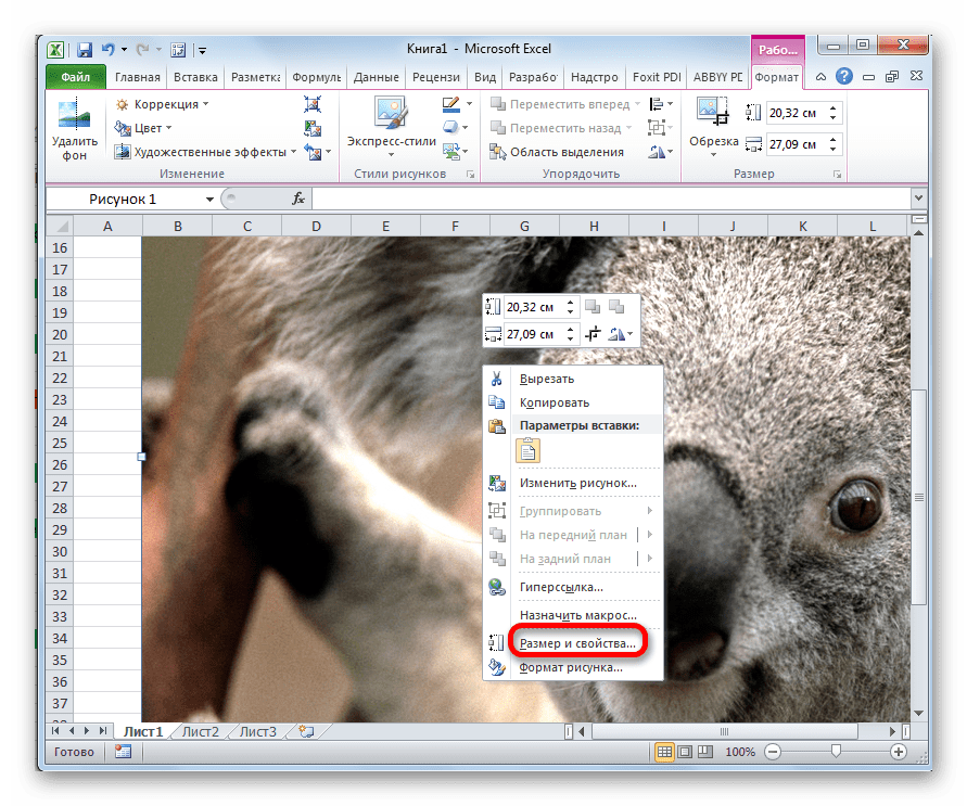
- Кликаем по изображению правой кнопкой мыши. Открываются параметры рисунка в виде контекстного меню. Кликаем по пункту «Размер и свойства».
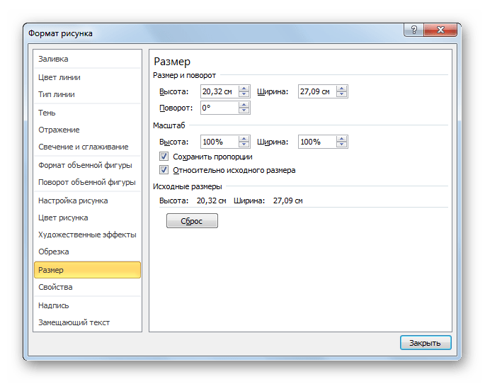
- Открывается окно, в котором присутствует множество инструментов по изменению свойств картинки. Тут можно изменить её размеры, цветность, произвести обрезку, добавить эффекты и сделать много другого. Всё зависит от конкретного изображения и целей, для которых оно используется.
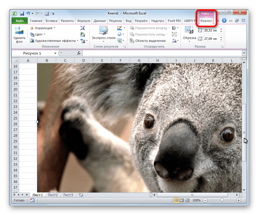
- Но в большинстве случаев нет необходимости открывать окно «Размеры и свойства», так как вполне хватает инструментов, которые предлагаются на ленте в дополнительном блоке вкладок «Работа с рисунками».
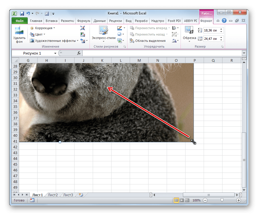
- Если мы хотим вставить изображение в ячейку, то самым важным моментом при редактировании картинки является изменение её размеров, чтобы они не были больше размеров самой ячейки. Изменить размер можно следующими способами:
- через контекстное меню;
- панель на ленте;
- окно «Размеры и свойства»;
- перетащив границы картинки с помощью мышки.
Прикрепление картинки
Но, даже после того, как изображение стало меньше ячейки и было помещено в неё, все равно оно осталось неприкрепленным. То есть, если мы, например, произведем сортировку или другой вид упорядочивания данных, то ячейки поменяются местами, а рисунок останется все на том же месте листа. Но, в Excel все-таки существуют некоторые способы прикрепления картинки. Рассмотрим их далее.

Способ 1: защита листа
Одним из способов прикрепить изображение является применение защиты листа от изменений.
- Подгоняем размер рисунка под размер ячейки и вставляем его туда, как было рассказано выше.
- Кликаем по изображению и в контекстном меню выбираем пункт «Размер и свойства».
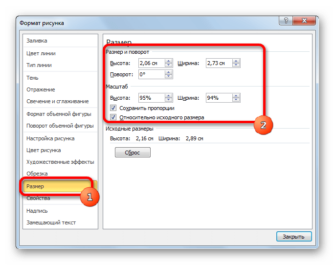
- Открывается окно свойств рисунка. Во вкладке «Размер» удостоверяемся, чтобы величина картинки была не больше размера ячейки. Также проверяем, чтобы напротив показателей «Относительно исходного размера» и «Сохранить пропорции» стояли галочки. Если какой-то параметр не соответствует указанному выше описанию, то изменяем его.
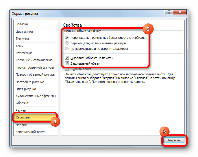
- Переходим во вкладку «Свойства» этого же окна. Устанавливаем галочки напротив параметров «Защищаемый объект» и «Выводить объект на печать», если они не установлены. Ставим переключатель в блоке настроек «Привязка объекта к фону» в позицию «Перемещать и изменять объект вместе с ячейками». Когда все указанные настройки выполнены, жмем на кнопку «Закрыть», расположенную в нижнем правом углу окна.
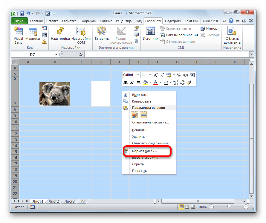
- Выделяем весь лист, нажатием сочетания клавиш Ctrl+A, и переходим через контекстное меню в окно настроек формата ячеек.
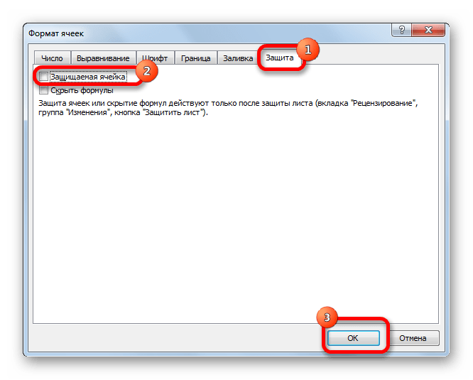
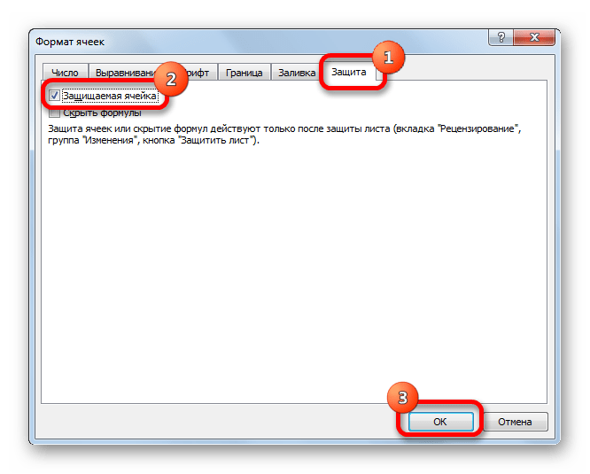
- Во вкладке «Защита» открывшегося окна снимаем галочку с параметра «Защищаемая ячейка» и жмем на кнопку «OK».
- Выделяем ячейку, где находится картинка, которую нужно закрепить. Открываем окно формата и во вкладке «Защита» устанавливаем галочку около значения «Защищаемая ячейка». Кликаем по кнопке «OK».
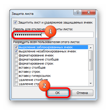
- Во вкладке «Рецензирование» в блоке инструментов «Изменения» на ленте кликаем по кнопке «Защитить лист».
- Открывается окошко, в котором вводим желаемый пароль для защиты листа. Жмем на кнопку «OK», а в следующем открывшемся окне снова повторяем введенный пароль.

После этих действий диапазоны, в которых находятся изображения, защищены от изменений, то есть, картинки к ним привязаны. В этих ячейках нельзя будет производить никаких изменений до снятия защиты. В других диапазонах листа, как и прежде, можно делать любые изменения и сохранять их. В то же время, теперь даже если вы решите провести сортировку данных, то картинка уже никуда не денется с той ячейки, в которой находится.
Урок: Как защитить ячейку от изменений в Excel
Способ 2: вставка изображения в примечание
Также можно привязать рисунок, вставив его в примечание.
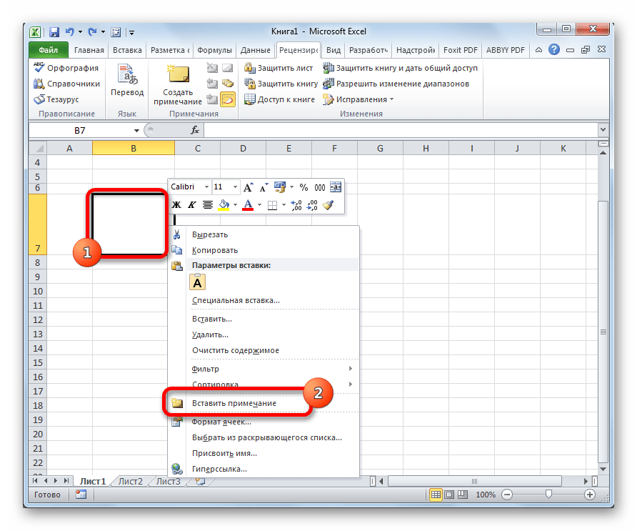
- Кликаем по ячейке, в которую планируем вставить изображение, правой кнопкой мышки. В контекстном меню выбираем пункт «Вставить примечание».
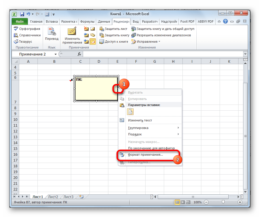
- Открывается небольшое окошко, предназначенное для записи примечания. Переводим курсор на его границу и кликаем по ней. Появляется ещё одно контекстное меню. Выбираем в нём пункт «Формат примечания».
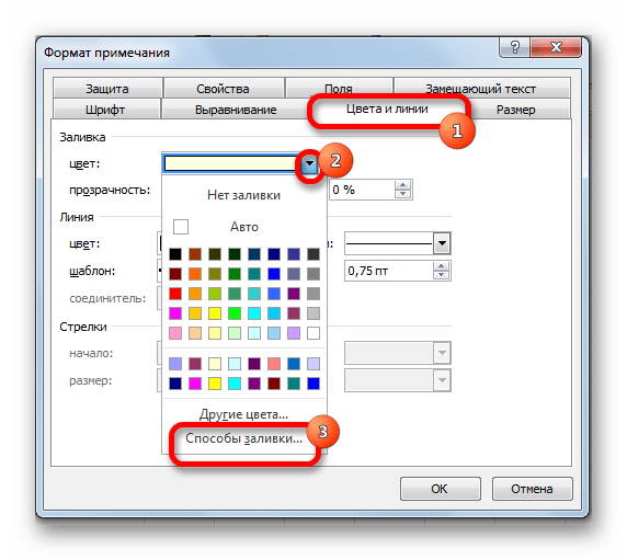
- В открывшемся окне настройки формата примечаний переходим во вкладку «Цвета и линии». В блоке настроек «Заливка» кликаем по полю «Цвет». В открывшемся перечне переходим по записи «Способы заливки…».
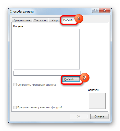
- Открывается окно способов заливки. Переходим во вкладку «Рисунок», а затем жмем на кнопку с одноименным наименованием.
- Открывается окно добавления изображения, точно такое же, как было описано выше. Выбираем рисунок и жмем на кнопку «Вставить».
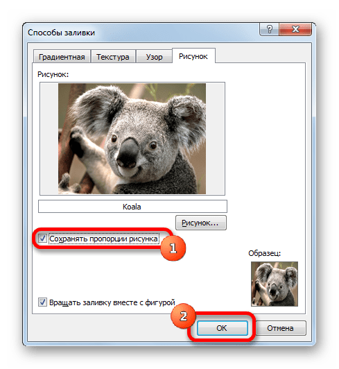
- Изображение добавилось в окно «Способы заливки». Устанавливаем галочку напротив пункта «Сохранять пропорции рисунка». Жмем на кнопку «OK».
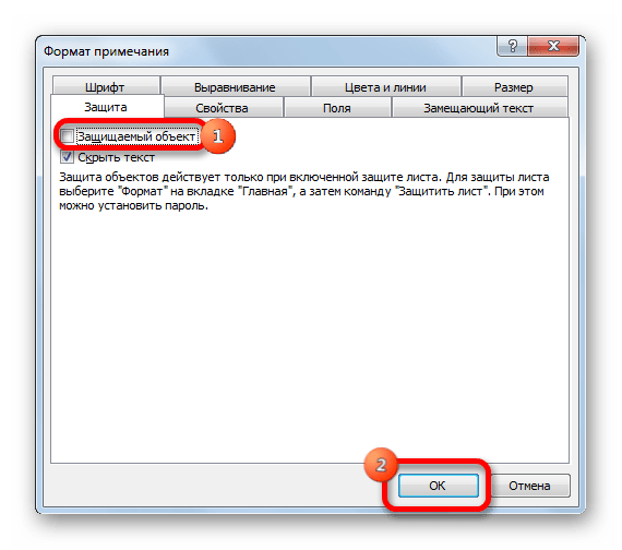
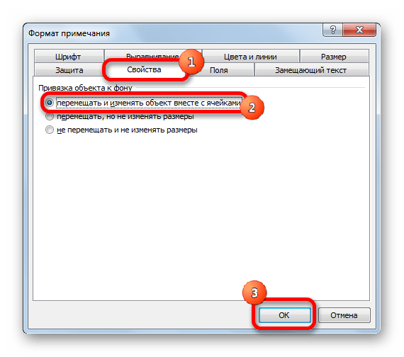
- После этого возвращаемся в окно «Формат примечания». Переходим во вкладку «Защита». Убираем галочку с параметра «Защищаемый объект».
- Переходим во вкладку «Свойства». Устанавливаем переключатель в позицию «Перемещать и изменять объект вместе с ячейками». Вслед за этим жмем на кнопку «OK».
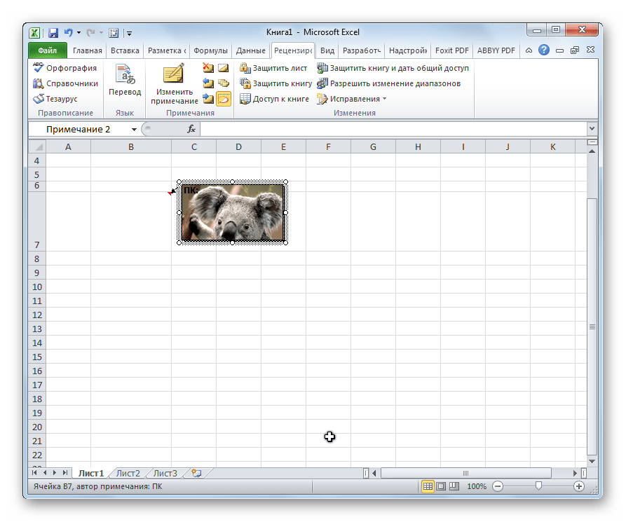
После выполнения всех вышеперечисленных действий, изображение не только будет вставлено в примечание ячейки, но и привязано к ней. Конечно, данный способ подходит не всем, так как вставка в примечание налагает некоторые ограничения.
Способ 3: режим разработчика
Привязать изображения к ячейке можно также через режим разработчика. Проблема состоит в том, что по умолчанию режим разработчика не активирован. Так что, прежде всего, нам нужно будет включить его.
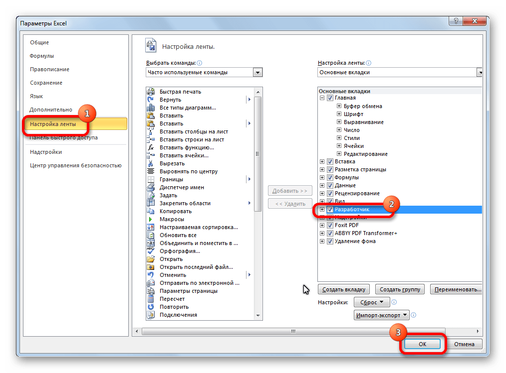
- Находясь во вкладке «Файл» переходим в раздел «Параметры».
- В окне параметров перемещаемся в подраздел «Настройка ленты». Устанавливаем галочку около пункта «Разработчик» в правой части окна. Жмем на кнопку «OK».
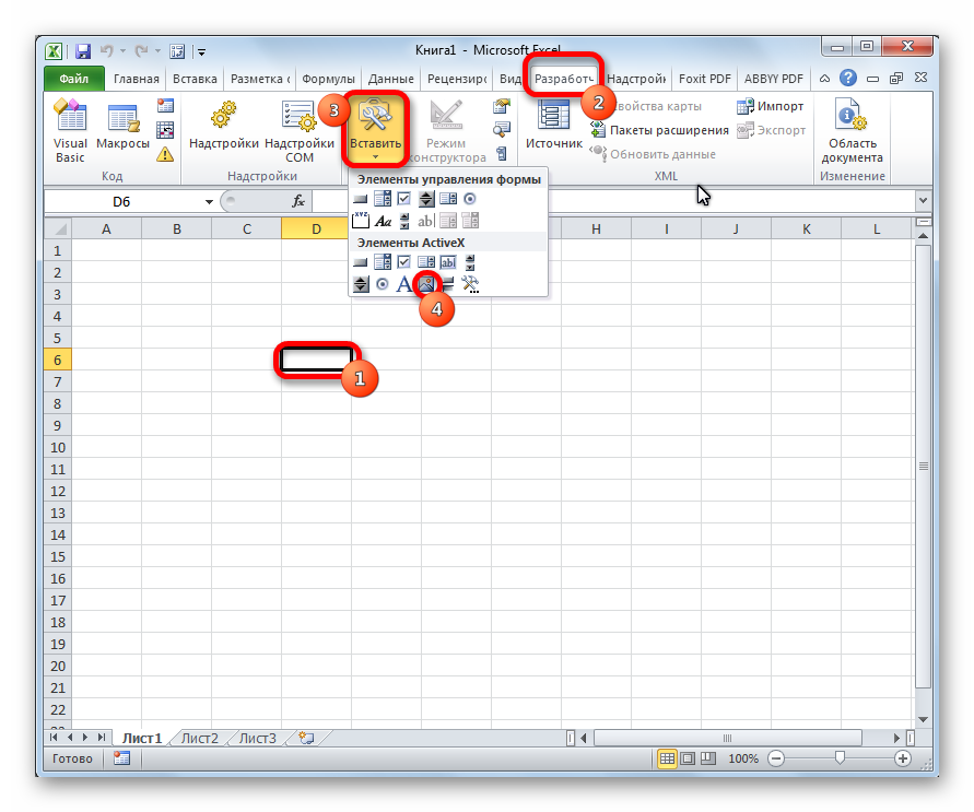
- Выделяем ячейку, в которую планируем вставить картинку. Перемещаемся во вкладку «Разработчик». Она появилась после того, как мы активировали соответствующий режим. Кликаем по кнопке «Вставить». В открывшемся меню в блоке «Элементы ActiveX» выбираем пункт «Изображение».
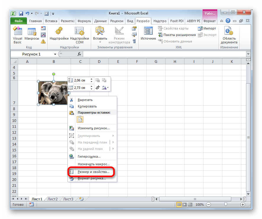
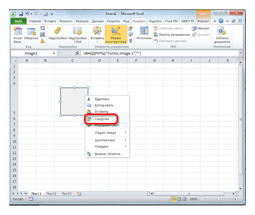
- Появляется элемент ActiveX в виде пустого четырехугольника. Регулируем его размеры перетаскиванием границ и помещаем в ячейку, где планируется разместить изображение. Кликаем правой кнопкой мыши по элементу. В контекстном меню выбираем пункт «Свойства».
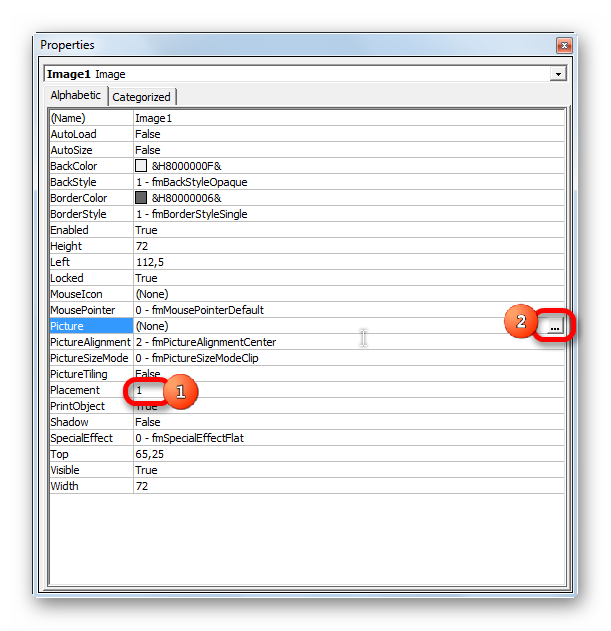
- Открывается окно свойств элемента. Напротив параметра «Placement» устанавливаем цифру «1» (по умолчанию «2»). В строке параметра «Picture» жмем на кнопку, на которой изображено многоточие.
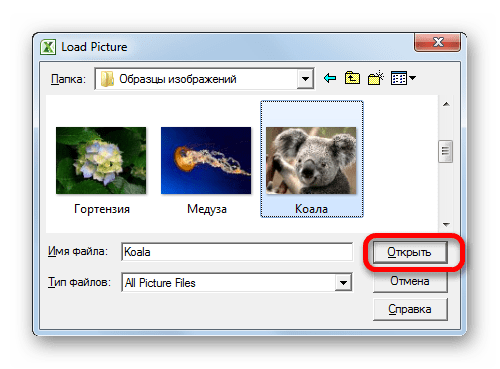
- Открывается окно вставки изображения. Ищем нужную картинку, выделяем её и жмем на кнопку «Открыть».
- После этого можно закрывать окно свойств. Как видим, рисунок уже вставлен. Теперь нам нужно полностью привязать его к ячейке. Выделяем картинку и переходим во вкладку «Разметка страницы». В блоке настроек «Упорядочить» на ленте жмем на кнопку «Выровнять». Из выпадающего меню выбираем пункт «Привязать к сетке». Затем чуть-чуть двигаем за край рисунка.

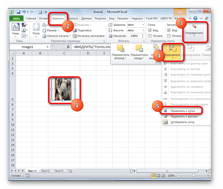
После выполнения вышеперечисленных действий картинка будет привязано к сетке и выбранной ячейке.
Как видим, в программе Эксель имеется несколько способов вставить изображение в ячейку и привязать его к ней. Конечно, способ со вставкой в примечание подойдет далеко не всем пользователям. А вот два остальных варианта довольно универсальны и каждый сам должен определиться, какой из них для него удобнее и максимально соответствует целям вставки.
![]()
Download Article
![]()
Download Article
Embedding images in your spreadsheets will add interest in your data and may help explain the results of your analyses to other users. You can add pictures, clip art and SmartArt to your Excel workbooks along with graphs that are created from charts. Are you ready to liven it up?
Steps
-
1
Launch the Microsoft Excel application installed on your computer.
-
2
Open the workbook file in which you want to add images.
Advertisement
-
3
Decide which type of image is best for your spreadsheet’s purpose.
- You may want to include a photograph of a beach or some clip art that represents outdoor leisure activities if your spreadsheet concerns activities available during the summer.
- You can add clip art showing a price tag or up and down arrows if your spreadsheet depicts the sales results following a recent price increase.
-
4
Click a blank cell in your worksheet to select it.
-
5
Insert the appropriate image into your spreadsheet.
- All types of images are found in the Insert menu or tab, depending on your version of Excel. Here, you can add pictures and other types of graphics.
- If you wish to add an image you have downloaded from the Internet or have saved on your hard drive, use the «Insert picture from file» option. Browse to the image saved on your computer and double-click it to insert.
- If you want to use clip art, select that option from the Insert menu and search for your clip art in the right pane. Clicking the clip art image will insert it into your spreadsheet.
-
6
Resize the image to fit the area you want to fill.
- Hover your mouse over a corner of the image until you see the resize cursor.
- Click and drag the corner of the image in toward the middle to shrink it; drag outward to enlarge.
-
7
Edit the properties of your image.
- Right-click on the image embedded in your worksheet and choose the Properties option from the pop-up menu.
- Add a border, shadow, 3D or other effects to your image.
-
8
Repeat the process to add more images to your worksheet.


Advertisement
Ask a Question
200 characters left
Include your email address to get a message when this question is answered.
Submit
Advertisement
Video
-
You can choose to slightly overlap your images by applying the correct layers to each one. Right-click on an image and choose the Send Backward or Send Forward options to layer your images.
Thanks for submitting a tip for review!
Advertisement
-
Be wary of undermining your credibility in professional situations with the use of excessive clip art. Whereas one image may add some interest to your work, you want the data to be the primary focus—not the clip art.
Advertisement
About This Article
Thanks to all authors for creating a page that has been read 259,434 times.
Is this article up to date?
Содержание
- Insert a Picture/Image in Excel Cell
- How to Insert a Picture/Image in Excel Cell?
- Change Image Size According to Cell Size in Excel
- How to Create an Excel Dashboard with Images?
- Things to Remember
- Recommended Articles
- How to insert picture in Excel cell, comment, header or footer
- How to insert picture in Excel
- Insert an image from a computer
- Add picture from the web, OneDrive or Facebook
- Paste picture in Excel from another program
- How to insert picture in Excel cell
- How to insert multiple pictures into cells in Excel
- How to insert picture in a comment
- A quick way to insert a picture in a comment
- How to embed image into Excel header or footer
- Insert a picture in Excel cell with formula
- Insert data from another sheet as picture
- How to copy/paste as picture in Excel
- Make a dynamic picture with Camera tool
- How to modify picture in Excel
- How to copy or move picture in Excel
- How to resize picture in Excel
- How to change picture’s colors and styles
- How to replace picture in Excel
- How to delete picture in Excel
Insert a Picture/Image in Excel Cell


How to Insert a Picture/Image in Excel Cell?
Table of contents
Inserting a picture or an image into an Excel cell is easy.
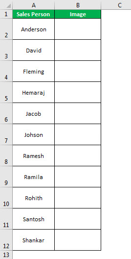
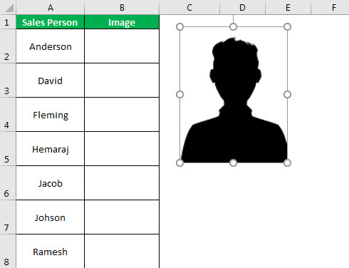
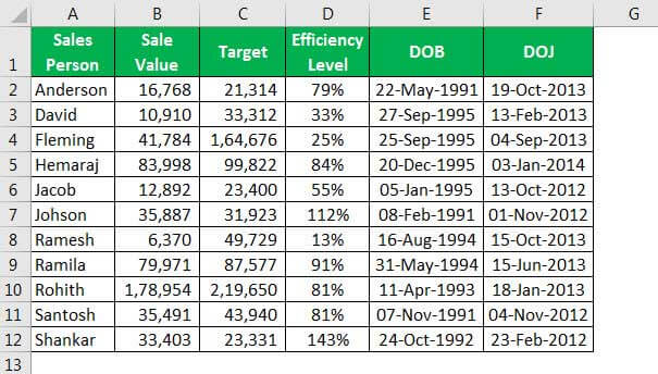
- For example, we have sales employees’ names in the Excel file. Below is the list.

We have their images on the computer hard disk.
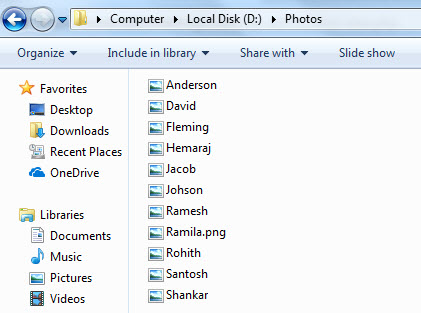
We want to bring the image against each person’s name, respectively.
Note: All the images are dummy. We can download them from Google directly.
We must copy the above list of names and paste it into Excel. Make the row height as 36 and column width in Excel 14.3.
Go to the Insert tab and click on Pictures.
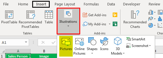
Once we click on Pictures, it asks us to choose the picture folder location from the computer. So, we must select the location and the pictures we want to insert.
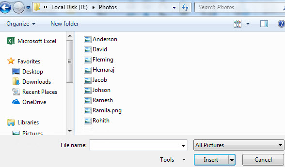
We can insert a picture one by one in an Excel cell, or we can insert it in one shot. To insert at one go, we need to be sure which represents who. So, we are going to insert them one by one. Select the image we want to insert and click on Insert.

Now, we can see the image in our Excel file.
This picture is not yet ready to use. We need to resize this. We must select the picture and resize it using the drag and drop option in Excel from the corner edges of the image, or we can resize the height and width under the Format tab.
Note: Modify the row height as 118 and column width as 26.

To fit the picture to the cell size, we must hold the ALT key and drag the picture corners. After that, it will automatically fit the cell size.
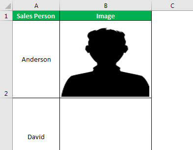
Like this, we must repeat this task for all the employees.
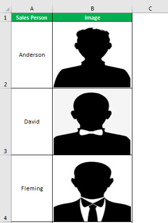
Change Image Size According to Cell Size in Excel
Now, we need to fit these images to the cell size. Whenever the cell width or height changes, the picture also should change accordingly.
- Step 1: First, we must select one image and press “Ctrl + A.” It will choose all the images in the active worksheet. (Make sure all the images are selected).
- Step 2:Now, press “Ctrl + 1.” It will open up the “Format” option on the right-hand side of the screen. Note: We are using Excel 2016 version.

- Step 3: Under “Format Picture,” select “Size & Properties.”
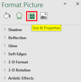
- Step 4: Click on “Properties” and select the option “Move and size with cells.”
- Step 5: We have locked the images to their respective cell sizes. It is dynamic now. As the cell changes, images are also kept changing.
How to Create an Excel Dashboard with Images?
We have created a master sheet that contains all the details of the employees.
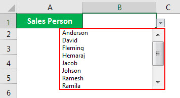
- Step 1: The sheet creates a dropdown list of employee lists in the dashboard.
- Step 2: We must Apply VLOOKUPApply VLOOKUPThe VLOOKUP excel function searches for a particular value and returns a corresponding match based on a unique identifier. A unique identifier is uniquely associated with all the records of the database. For instance, employee ID, student roll number, customer contact number, seller email address, etc., are unique identifiers.read more to get the “Sales Value,” “Target,” “Efficiency Level,” “DOB,” and “DOJ” from the “Employee Details” sheet.
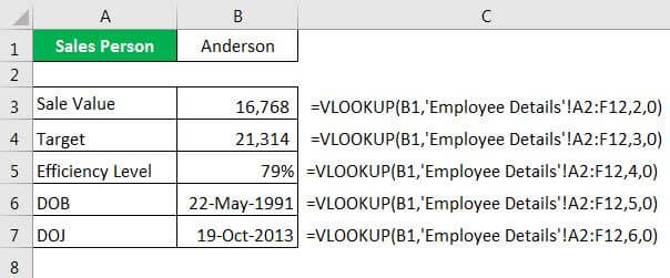
The values will be automatically updated as you change the name from the drop-down.
- Step 3: The big part is getting the employee’s photo selected from the drop-down. For this, we need to create a “Name Manager.”
Go to “FORMULAS” > “Define Name” in Excel.
Things to Remember
- We must make the image adjustment that fits or changes the cell movement.
- Create a master sheet containing all the consolidated data to create a dashboard.
- We must use the “ALT” key to adjust the image to the extreme corners of the cell.
Recommended Articles
This article is a guide to Insert a Picture/Image in Excel Cell. We discussed inserting a picture or an image into a cell in Excel and creating a dashboard with images in Excel, an example, and a downloadable Excel sheet. You can learn more about Excel from the following articles: –
Источник
 by Svetlana Cheusheva, updated on March 20, 2023
The tutorial shows different ways to insert an image in Excel worksheet, fit a picture in a cell, add it to a comment, header or footer. It also explains how to copy, move, resize or replace an image in Excel.
While Microsoft Excel is primarily used as a calculation program, in some situations you may want to store pictures along with data and associate an image with a particular piece of information. For example, a sales manager setting up a spreadsheet of products may want to include an extra column with product images, a real estate professional may wish to add pictures of different buildings, and a florist would definitely want to have photos of flowers in their Excel database.
In this tutorial, we will look at how to insert image in Excel from your computer, OneDrive or from the web, and how to embed a picture into a cell so that it adjusts and moves with the cell when the cell is resized, copied or moved. The below techniques work in all versions of Excel 2010 — Excel 365.
How to insert picture in Excel
All versions of Microsoft Excel allow you to insert pictures stored anywhere on your computer or another computer you are connected to. In Excel 2013 and higher, you can also add an image from web pages and online storages such as OneDrive, Facebook and Flickr.
Insert an image from a computer
Inserting a picture stored on your computer into your Excel worksheet is easy. All you have to do is these 3 quick steps:
- In your Excel spreadsheet, click where you want to put a picture.
- Switch to the Insert tab >Illustrations group, and click Pictures.
- In the Insert Picture dialog that opens, browse to the picture of interest, select it, and click Insert. This will place the picture near the selected cell, more precisely, the top left corner of the picture will align with the top left corner of the cell.

To insert several images at a time, press and hold the Ctrl key while selecting pictures, and then click Insert, like shown in the screenshot below: 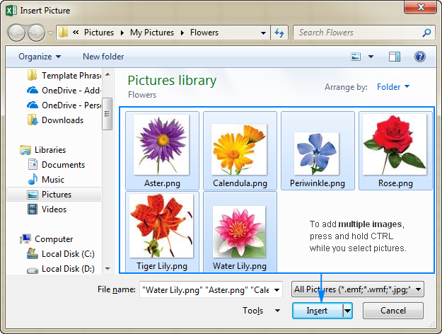
Done! Now, you can re-position or resize your image, or you can lock the picture to a certain cell in a way that it resizes, moves, hides and filters together with the associated cell.
Add picture from the web, OneDrive or Facebook
In the recent versions of Excel 2016 or Excel 2013, you can also add images from web-pages by using Bing Image Search. To have it done, perform these steps:
- On the Insert tab, click the Online Pictures button:
- The following window will appear, you type what you’re looking for into the search box, and hit Enter:
- In search results, click on the picture you like best to select it, and then click Insert. You can also select a few images and have them inserted in your Excel sheet in one go:


If you are looking for something specific, you can filter the found images by size, type, color or license — just use one or more filters at the top of the search results.
Note. If you plan to distribute your Excel file to someone else, check the picture’s copyright to make sure you can legally use it.
Besides adding images from Bing search, you can insert a picture stored on your OneDrive, Facebook or Flickr. For this, click the Online Pictures button on the Insert tab, and then do one of the following:
- Click Browse next to OneDrive, or
- Click the Facebook or Flickr icon at the bottom of the window.

Note. If your OneDrive account does not appear in the Insert Pictures window, most likely you are not signed in with your Microsoft account. To fix this, click the Sign in link at the upper right corner of the Excel window.
Paste picture in Excel from another program
The easiest way to insert a picture in Excel from another application is this:
- Select an image in another application, for example in Microsoft Paint, Word or PowerPoint, and click Ctrl + C to copy it.
- Switch back to Excel, select a cell where you want to put the image and press Ctrl + V to paste it. Yep, it’s that easy!

How to insert picture in Excel cell
Normally, an image inserted in Excel lies on a separate layer and «floats» on the sheet independently from the cells. If you want to embed an image into a cell, change the picture’s properties as shown below:
- Resize the inserted picture so that it fits properly within a cell, make the cell bigger if needed, or merge a few cells.
- Right-click the picture and select Format Picture…
- On the Format Picture pane, switch to the Size & Properties tab, and select the Move and size with cells option.


That’s it! To lock more images, repeat the above steps for each image individually. You can even put two or more images into one cell if needed. As a result, you will have a beautifully organized Excel sheet where each image is linked to a particular data item, like this: 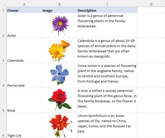
Now, when you move, copy, filter or hide the cells, the pictures will also be moved, copied, filtered or hidden. The image in the copied/moved cell will be positioned the same way as the original.
How to insert multiple pictures into cells in Excel
As you have just seen, it’s quite easy to add a picture in an Excel cell. But what if you have a dozen different images to insert? Changing the properties of each picture individually would be a waste of time. With our Ultimate Suite for Excel, you can have the job done in seconds.
- Select the left top cell of the range where you want to insert pictures.
- On the Excel ribbon, go to the Ablebits Tools tab >Utilities group, and click the Insert Picture button.
- Choose whether you want to arrange pictures vertically in a column or horizontally in a row, and then specify how you want to fit images:
- Fit to Cell — resize each picture to fit the size of a cell.
- Fit to Image — adjust each cell to the size of a picture.
- Specify Height — resize the picture to a specific height.
- Select the pictures you want to insert and click the Open button.

Note. For pictures inserted in this way, the Move but don’t size with cells option is selected, meaning the pictures will keep their size when you move or copy cells.
Inserting an image into an Excel comment may often convey your point better. To have it done, please follow these steps:
- Create a new comment in the usual way: by clicking New Comment on the Review tab, or selecting Insert Comment from the right-click menu, or pressing Shift + F2 .
- Right click the border of the comment, and choose Format Comment… from the context menu.
If you are inserting a picture into an existing comment, click Show All Comments on the Review tab, and then right-click the border of the comment of interest. 

If you want to Lock picture aspect ratio, select the corresponding checkbox like shown in the screenshot below: 
The picture has been embedded into the comment and will show up when you hover over the cell: 
If you’d rather not waste your time on routine tasks like this, Ultimate Suite for Excel can save a few more minutes for you. Here’s how:
- Select a cell where you want to add a comment.
- On the Ablebits Tools tab, in the Utilities group, click Comments Manager >Insert Picture.
- Select the image you want to insert and click Open. Done!

In situations when you want to add a picture into the header or footer of your Excel worksheet, proceed with the following steps:
- On the Insert tab, in the Text group, click Header & Footer. This should take you to the Header & Footer tab.
- To insert a picture in the header, click a left, right or center header box. To insert a picture in the footer, first click the text «Add footer», and then click within one of the three boxes that will appear.
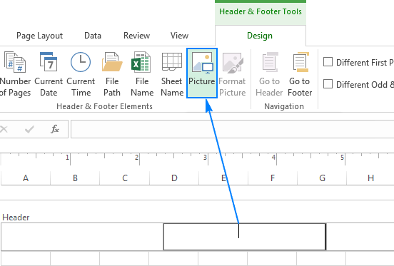
- On the Header & Footer tab, in the Header & Footer Elements group, click Picture.
- The Insert Pictures dialog window will pop up. You browse to the picture you want to add and click Insert. The &[Picture] placeholder will appear in the header box. As soon as you click anywhere outside of the header box, the inserted picture will appear:

Insert a picture in Excel cell with formula
Microsoft 365 subscribers have one more exceptionally easy way to insert a picture in cells — the IMAGE function. All you need to do is:
- Upload your image to any website with the «https» protocol in any of these formats: BMP, JPG/JPEG, GIF, TIFF, PNG, ICO, or WEBP.
- Insert an IMAGE formula into a cell.
- Press the Enter key. Done!
The image immediately appears in a cell. The size is adjusted automatically to fit into the cell maintaining the aspect ratio. It’s also possible to fill the entire cell with the image or set given width and height. When you hover over the cell, a bigger tooltip will pop up. 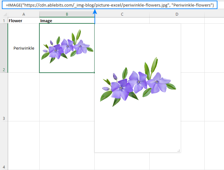
Insert data from another sheet as picture
As you have just seen, Microsoft Excel provides a numbers of different ways to insert an image into a cell or in a specific area of a worksheet. But did you know you can also copy information from one Excel sheet and insert it in another sheet as an image? This technique comes in handy when you are working on a summary report or assembling data from several worksheets for printing.
Overall, there are two methods to insert Excel data as picture:
Copy as Picture option — allows copy/pasting information from another sheet as a static image.
Camera tool — inserts data from another sheet as a dynamic picture that updates automatically when the original data changes.
How to copy/paste as picture in Excel
To copy Excel data as an image, select the cells, chart(s) or object(s) of interest and do the following.
- On the Home tab, in the Clipboard group, click the little arrow next to Copy, and then click Copy as Picture…
- Choose whether you want to save the copied contents As shown on screen or As shown when printed, and click OK:
- On another sheet or in a different Excel document, click where you want to put the picture and press Ctrl + V .


That’s it! The data from one Excel worksheet is pasted into another sheet as a static picture.
Make a dynamic picture with Camera tool
To begin with, add the Camera tool to your Excel ribbon or Quick Access Toolbar as explained here. 
With the Camera button in place, perform the following steps to take a photo of any Excel data including cells, tables, charts, shapes, and the like:
- Select a range of cells to be included in the picture. To capture a chart, select the cells surrounding it.
- Click on the Camera icon.
- In another worksheet, click where you want to add a picture. That’s all there is to it!
Unlike the Copy as Picture option, Excel Camera creates a «live» image that synchronizes with the original data automatically.
How to modify picture in Excel
After inserting a picture in Excel what is the first thing you’d usually want to do with it? Position properly on the sheet, resize to fit into a cell, or maybe try some new designs and styles? The following sections demonstrate some of the most frequent manipulations with images in Excel.
How to copy or move picture in Excel
To move an image in Excel, select it and hover the mouse over the picture until the pointer changes into the four-headed arrow, then you can click the image and drag it anywhere you want: 
To adjust the position of a picture in a cell, press and hold the Ctrl key while using the arrows keys to reposition the picture. This will move the image in small increments equal to the size of 1 screen pixel.
To move an image to a new sheet or workbook, select the image and press Ctrl + X to cut it, then open another sheet or a different Excel document and press Ctrl + V to paste the image. Depending on how far you’d like to move an image in the current sheet, it may also be easier to use this cut/paste technique.
To copy a picture to clipboard, click on it and press Ctrl + C (or right-click the picture, and then click Copy). After that, navigate to where you wish to place a copy (in the same or in a different worksheet), and press Ctrl + V to paste the picture.
How to resize picture in Excel
The easiest way to resize an image in Excel is to select it, and then drag in or out by using the sizing handles. To keep the aspect ratio intact, drag one of the corners of the image. 
Another way to resize a picture in Excel is to type the desired height and width in inches in the corresponding boxes on the Picture Tools Format tab, in the Size group. This tab appears on the ribbon as soon as you select the picture. To preserve the aspect ratio, type just one measurement and let Excel change the other automatically. 
How to change picture’s colors and styles
Of course, Microsoft Excel does not have all the capabilities of photo editing software programs, but you may be surprised to know how many different effects you can apply to images directly in your worksheets. For this, select the picture, and navigate to the Format tab under Picture Tools: 
Here is a short overview of the most useful format options:
- Remove the image background (Remove Background button in the Adjust group).
- Improve the brightness, sharpness or contrast of the picture (Corrections button in the Adjust group).
- Adjust the image colors by changing saturation, tone or do complete recoloring (Color button in the Adjust group).
- Add some artistic effects so that your image looks more like a painting or sketch (Artistic Effects button in the Adjust group).
- Apply special picture styles such as 3-D effect, shadows, and reflections (Picture Styles group).
- Add or remove the picture borders (Picture Border button in the Picture Styles group).
- Reduce the image file size (Compress Pictures button in the Adjust group).
- Crop the picture to remove unwanted areas (Crop button in the Size group)
- Rotate the picture at any angle and flip it vertically or horizontally (Rotate button in the Arrange group).
- And more!
To restore the original size and format of the image, click the Reset Picture button in the Adjust group.
How to replace picture in Excel
To replace an existing picture with a new one, right-click it, and then click Change Picture. Choose whether you want to insert a new picture from a file or online sources,
locate it, and click Insert: 
The new picture will be placed exactly in the same position as the old one and will have the same formatting options. For example, if the previous picture was inserted into a cell, the new one will also be.
How to delete picture in Excel
To delete a single picture, simply select it and press the Delete button on your keyboard.
To delete several pictures, press and hold Ctrl while you select images, and then press Delete.
To delete all pictures on the current sheet, use the Go To Special feature in this way:
- Press F5 key to open the Go To dialog box.
- Click the Special… button at the bottom.
- In the Go To Special dialog, check the Object option, and click OK. This will select all pictures on the active worksheet, and you press the Delete key to delete them all.

Note. Please be very careful when using this method because it selects all objects including pictures, shapes, WordArt, etc. So, before pressing Delete, make sure the selection does not contain some objects that you’d like to keep.
This is how you insert and work with pictures in Excel. I hope you will find the information helpful. Anyway, I thank you for reading and hope to see you on our blog next week!
Источник