Insert no value in excel - Word и Excel - помощь в работе с программами

Why not just check for the value being «» rather than empty?

Of course your formula will show division by 0 error if B1 is empty or 0.

I guess you could use a UDF like this but a simple If would do just as well.

Code:

'=If(ISE(A1),"",A1) or =If(A1="","",A1)
Function ISE(cell As Range) As Boolean
  If cell.Value = "" Then
    ISE = True
    Else: ISE = False
  End If
End Function

I’ll ask my question another way…

I’ve learned that VBA includes a Null value in the variable vbNullString

I’ve tested running a macro to insert a null value into a cell using vbNullString and it works… that is, it inserts a null value as follows…
Sub InsertNull_IfDivisiorZero()
If B1 = «» Then
ActiveCell.Value = vbNullString
Else
ActiveCell.Value = A1 / B1
End If
End Sub

However, when I create a UDF as follows…
Function NullValue()
ActiveCell.Value = vbNullString
End Function

and include this UDF in a cell formula as follows…
=IF(B1=»»,NullValue(),A1/B1)

the result is #VALUE! error with the explanation…
A value used in the formaul is of a wrong data type.

AND SO, I ask my question again…
«How can a Null Value be inserted into a cell in a formula?»

Not sure what this is accomplishing, but your Function is not written correctly:

Code:

Function NullValue() As String
NullValue = vbNullString
End Function

WHy not just check to see if you are trying to divide by a non-zero number?

=IF(B1,A1/B1,»»)

Last edited: Aug 8, 2008

Several points

1 —

Your UDF is wrong. You cannot assign values to cells in a UDF. Your statement is not allowed.
If you want to return the null string then use Hotpepper’s :

Code:

Function NullValue()
    NullValue = vbNullString
End Function

Now you could use:

=IF(B1=»»,NullValue(),A1/B1)

This is, however, equivalent to:

=IF(B1=»»,»»,A1/B1)

no need for the UDF, and does not solve your problem (b1 can be 0).

2 — «I’ve learned that VBA includes a Null value in the variable vbNullString»

No, vbNullString is not the vba Null value, it’s a constant equivalent to an empty string. You cannot write a null value to a cell. You use an empty string instead, like in the previous point.

3 —

ISBLANK() tests if a cell is empty. As far as I can see in your examples your cells have formulas and so will never be empty and so you have no use ffor ISBLANK() in this case.

Note that COUNTBLANK(), has a different criterion: it counts not only empty cell but also cells with empty strings.

4 —

In your formula you don’t want to perform the division if either

— the cell is empty
— the cell has a null string
— the cell has the value 0 (zero)

use:

=IF(N(B1),A1/B1,»»)

It works for the 3 cases.

Another option that will catch other problems:
=IF(ISERROR(A1/B1),»»,A1/B1)

I thank everyone for their input. However, the responses have not addressed my main need, which is to insert a NULL VALUE that is something other than «».

Perhaps by posting a couple of files that you can examine you’ll better understand what I’m trying to do.

At http://dplum.com/excel you will find a PDF file that can be reviewed (if you’d prefer to not open an xls file). Or you can examine the xls file from which the PDF was created.

Please note:
1. The Batting Average field is calulated using =IF(C6=0,»»,D6/C6) to avoid a Divide by Zero Error.
2. The IF statement in the Comment field (to show Avg > .350 as a «Slugger!») results in 2 errors… cells F11, F13… these cells display «Slugger!» even though they have a Double Quote («») Null Value in them.
3. To fix this error I need to use the AND() function to also check that the cell is Not = «»

So… if a TRUE Null Value could be placed in these cells rather than the «» the error would not happen. IS THERE A WAY TO DO THIS?

No, you can’t have nothing in a cell and a formula.

But this should be a very easy fix.

In F6:
=IF(N(E6)>0.35,»Slugger!»,»»)

Copy down.

Hotpepper,
Thanks for your feedback.

Hi, Dennis.

Seems like you have sorted out the question.

I wanted to mention that a null (from dataset) can be written into a cell using Excel’s database type functionality — so a query table, or an ADO recordset copied to the worksheet.

Regards, Fazza

Источник

You may have a personal preference to display zero values in a cell, or you may be using a spreadsheet that adheres to a set of format standards that requires you to hide zero values. There are several ways to display or hide zero values.

Sometimes you might not want zero (0) values showing on your worksheets, sometimes you need them to be seen. Whether your format standards or preferences call for zeroes showing or hidden, there are several ways to make it happen.

Hide or display all zero values on a worksheet

Click File > Options > Advanced.
Under Display options for this worksheet, select a worksheet, and then do one of the following:
- To display zero (0) values in cells, check the Show a zero in cells that have zero value check box.
- To display zero (0) values as blank cells, uncheck the Show a zero in cells that have zero value check box.

Hide zero values in selected cells

These steps hide zero values in selected cells by using a number format. The hidden values appear only in the formula bar and are not printed. If the value in one of these cells changes to a nonzero value, the value will be displayed in the cell, and the format of the value will be similar to the general number format.

Select the cells that contain the zero (0) values that you want to hide.
You can press Ctrl+1, or on the Home tab, click Format > Format Cells.
Click Number > Custom.
In the Type box, type 0;-0;;@, and then click OK.

To display hidden values:

Select the cells with hidden zeros.
You can press Ctrl+1, or on the Home tab, click Format > Format Cells.
Click Number > General to apply the default number format, and then click OK.

Hide zero values returned by a formula

Select the cell that contains the zero (0) value.
On the Home tab, click the arrow next to Conditional Formatting > Highlight Cells Rules Equal To.
In the box on the left, type 0.
In the box on the right, select Custom Format.
In the Format Cells box, click the Font tab.
In the Color box, select white, and then click OK.

Display zeros as blanks or dashes

Use the IF function to do this.

Use a formula like this to return a blank cell when the value is zero:

=IF(A2-A3=0,””,A2-A3)

Here’s how to read the formula. If 0 is the result of (A2-A3), don’t display 0 – display nothing (indicated by double quotes “”). If that’s not true, display the result of A2-A3. If you don’t want the cells blank but want to display something other than 0, put a dash “-“ or other character between the double quotes.

Hide zero values in a PivotTable report

Click the PivotTable report.
On the Analyze tab, in the PivotTable group, click the arrow next to Options, and then click Options.
Click the Layout & Format tab, and then do one or more of the following:
- Change error display Check the For error values show check box under Format. In the box, type the value that you want to display instead of errors. To display errors as blank cells, delete any characters in the box.
- Change empty cell display Check the For empty cells show check box. In the box, type the value that you want to display in empty cells. To display blank cells, delete any characters in the box. To display zeros, clear the check box.

Top of Page

Display or hide all zero values on a worksheet

Click File > Options > Advanced.
Under Display options for this worksheet, select a worksheet, and then do one of the following:
- To display zero (0) values in cells, select the Show a zero in cells that have zero value check box.
- To display zero values as blank cells, clear the Show a zero in cells that have zero value check box.

Use a number format to hide zero values in selected cells

Follow this procedure to hide zero values in selected cells. If the value in one of these cells changes to a nonzero value, the format of the value will be similar to the general number format.

Select the cells that contain the zero (0) values that you want to hide.
You can use Ctrl+1, or on the Home tab, click Format > Format Cells.
In the Category list, click Custom.
In the Type box, type 0;-0;;@

Notes:

The hidden values appear only in the formula bar — or in the cell if you edit within the cell — and are not printed.
To display hidden values again, select the cells, and then press Ctrl+1, or on the Home tab, in the Cells group, point to Format, and click Format Cells. In the Category list, click General to apply the default number format. To redisplay a date or a time, select the appropriate date or time format on the Number tab.

Use a conditional format to hide zero values returned by a formula

Select the cell that contains the zero (0) value.
On the Home tab, in the Styles group, click the arrow next to Conditional Formatting, point to Highlight Cells Rules, and then click Equal To.
In the box on the left, type 0.
In the box on the right, select Custom Format.
In the Format Cells dialog box, click the Font tab.
In the Color box, select white.

Use a formula to display zeros as blanks or dashes

To do this task, use the IF function.

Example

The example may be easier to understand if you copy it to a blank worksheet.


1
2
3
4
5
6
7

A	B
Data
10
10
Formula	Description (Result)
=A2-A3	Second number subtracted from the first (0)
=IF(A2-A3=0,»»,A2-A3)	Returns a blank cell when the value is zero (blank cell)
=IF(A2-A3=0,»-«,A2-A3	Returns a dash when the value is zero (-)

For more information about how to use this function, see IF function.

Hide zero values in a PivotTable report

Click the PivotTable report.
On the Options tab, in the PivotTable Options group, click the arrow next to Options, and then click Options.
Click the Layout & Format tab, and then do one or more of the following:

Change error display Select the For error values, show check box under Format. In the box, type the value that you want to display instead of errors. To display errors as blank cells, delete any characters in the box.

Change empty cell display Select the For empty cells, show check box. In the box, type the value that you want to display in empty cells. To display blank cells, delete any characters in the box. To display zeros, clear the check box.

Top of Page

Display or hide all zero values on a worksheet

Click the Microsoft Office Button , click Excel Options, and then click the Advanced category.
Under Display options for this worksheet, select a worksheet, and then do one of the following:
- To display zero (0) values in cells, select the Show a zero in cells that have zero value check box.
- To display zero values as blank cells, clear the Show a zero in cells that have zero value check box.

Use a number format to hide zero values in selected cells

Follow this procedure to hide zero values in selected cells. If the value in one of these cells changes to a nonzero value, the format of the value will be similar to the general number format.

Select the cells that contain the zero (0) values that you want to hide.
You can press Ctrl+1, or on the Home tab, in the Cells group, click Format > Format Cells.
In the Category list, click Custom.
In the Type box, type 0;-0;;@

Notes:

The hidden values appear only in the formula bar — or in the cell if you edit within the cell — and are not printed.
To display hidden values again, select the cells, and then on the Home tab, in the Cells group, point to Format, and click Format Cells. In the Category list, click General to apply the default number format. To redisplay a date or a time, select the appropriate date or time format on the Number tab.

Use a conditional format to hide zero values returned by a formula

Select the cell that contains the zero (0) value.
On the Home tab, in the Styles group, click the arrow next to Conditional Formatting > Highlight Cells Rules > Equal To.
In the box on the left, type 0.
In the box on the right, select Custom Format.
In the Format Cells dialog box, click the Font tab.
In the Color box, select white.

Use a formula to display zeros as blanks or dashes

To do this task, use the IF function.

Example

The example may be easier to understand if you copy it to a blank worksheet.

How do I copy an example?

Select the example in this article.

Important: Do not select the row or column headers.

Selecting an example from Help

Press CTRL+C.
In Excel, create a blank workbook or worksheet.
In the worksheet, select cell A1, and press CTRL+V.

Important: For the example to work properly, you must paste it into cell A1 of the worksheet.

To switch between viewing the results and viewing the formulas that return the results, press CTRL+` (grave accent), or on the Formulas tab > Formula Auditing group > Show Formulas.

After you copy the example to a blank worksheet, you can adapt it to suit your needs.


1
2
3
4
5
6
7

A	B
Data
10
10
Formula	Description (Result)
=A2-A3	Second number subtracted from the first (0)
=IF(A2-A3=0,»»,A2-A3)	Returns a blank cell when the value is zero (blank cell)
=IF(A2-A3=0,»-«,A2-A3	Returns a dash when the value is zero (-)

For more information about how to use this function, see IF function.

Hide zero values in a PivotTable report

Click the PivotTable report.
On the Options tab, in the PivotTable Options group, click the arrow next to Options, and then click Options.
Click the Layout & Format tab, and then do one or more of the following:

Change error display Select the For error values, show check box under Format. In the box, type the value that you want to display instead of errors. To display errors as blank cells, delete any characters in the box.

Change empty cell display Select the For empty cells, show check box. In the box, type the value that you want to display in empty cells. To display blank cells, delete any characters in the box. To display zeros, clear the check box.

Why Do You Need A Blank Value Choice?

Sometimes you may come across instances where you want to include an option for your users to select a bank/empty value in a Data Validation drop-down list. This is definitely a “nice-to-have” tweak as users can simply hit their Delete or Backspace key to clear out the cell value. However, I have found this slight enhancement can make the user experience flow a bit more nicely as there could be doubt on the user’s end if they are allowed to have a blank value.

Let’s look at two ways you can get that blank value added into your Data Validation drop-down list. We will explore

Manually typing out the list choices
Referencing a cell range to pull in the list choices

Typing Out The List Values

A lesser-known feature of Data Validation Lists is that you can actually hardcode the values you want to display in your list. I typically prefer this route if I don’t want to risk someone accidentally changing the list options or if the list is containing something simple like yes/no options. Instead of referencing a cell range address, you can simply type the value you want to be listed and separate them with a comma.

The oddity though is that the universal value for blank in Excel (» «) DOES NOT give us a blank result in the data validation list. For one reason or another, you have to use two dashes to achieve this effect (—).

Excel Example Data Validation Drop-Down List

Please note, that even though the dashes show up as the selectable option in the drop-down menu, once selected, the cell value is empty/blank. The value will also be recognized as a blank value if pointed to in formulas.

Pulling Values From A Cell Range

If you want to use a range reference to populate your Data Validation List, you simply need to ensure the first row in your reference does not have a cell value. This will carry through to what is displayed in your drop-down menu.

Excel Example Data Validation Drop-Down List

I Hope This Helped!

Hopefully, I was able to explain how you can achieve the effect of having a no-value/empty option for your users to select in Data Validation drop-down lists. If you have any questions about this technique or suggestions on how to improve it, please let me know in the comments section below.

About The Author

Hey there! I’m Chris and I run TheSpreadsheetGuru website in my spare time. By day, I’m actually a finance professional who relies on Microsoft Excel quite heavily in the corporate world. I love taking the things I learn in the “real world” and sharing them with everyone here on this site so that you too can become a spreadsheet guru at your company.

Through my years in the corporate world, I’ve been able to pick up on opportunities to make working with Excel better and have built a variety of Excel add-ins, from inserting tickmark symbols to automating copy/pasting from Excel to PowerPoint. If you’d like to keep up to date with the latest Excel news and directly get emailed the most meaningful Excel tips I’ve learned over the years, you can sign up for my free newsletters. I hope I was able to provide you some value today and hope to see you back here soon! — Chris

Источник

I’m a complete newcomer to VBA so bear with me.

I have a list of consecutive integers with some values missing, also a list of missing values. These are columns A and B. What I’d like to be able to do is to search the list for the number that’s one smaller than the value in the selected cell, insert a cell just below that number, and put the selected value into the new cell, then delete from the «missing values» list.

For example:
Say I have, in column A, the list: (1 2 3 5 6 9 10)
And in column B: (4 7
What I’d like to be able to do is select the cell with «4» in it in column B, and have a sub that will:
1. Search the list in column A to find the cell containing «3»
2. Insert a cell in column A below the one containing «3», shifting the remainder down
3. Put «4» into the new column-A cell
4. Delete the cell containing «4» from column B, shifting the remainder up

I have over-simplified it … I would like to do this with code because in reality my column-A list has nearly 10,000 entries, and my missing-value column-B list contains a few hundred.

I might be able to figure it on my own, but would appreciate something I didn’t have to take weeks to tweak. Seems like if I knew more VBA it wouldn’t be that difficult … someday!

Источник

Watch Video – Insert Blank Row After Every Row in Excel

People who work with large data sets often need simple things such as inserting/deleting rows or columns.

While there are already many different (and simple) ways to add rows in Excel, when it comes to inserting a blank row after every other row (or every third or fourth row), things get a bit complicated.

Insert a Blank Row After Every Other Row

In this tutorial, I will show you some really simple ways to insert a blank row after every row in the existing dataset (or every nth row).

Since there is no direct way to add rows in between rows, the method covered in this article are workarounds to make this happen, And if you’re comfortable with VBA, then you can do this with a single click.

Using Helper Column and the Sort Feature

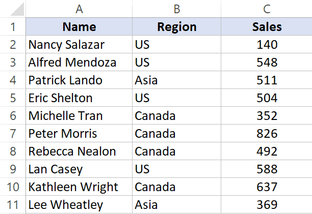
Suppose you have a dataset as shown below and you want to insert a blank between the existing rows.

Below are the steps to insert blank rows between existing rows:

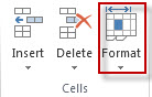
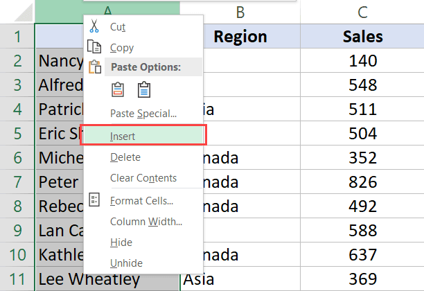
Insert a blank column to the left of the dataset. To do this, right-click on the column header of the left-most column and click on Insert.
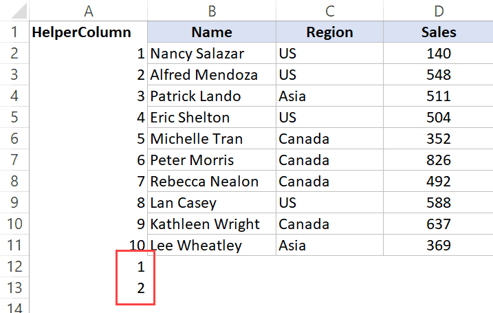
Enter the text ‘HelperColumn’ in A1 (you can use any text you want)
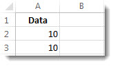
Enter 1 in cell A2 and 2 in cell A3.
Select both the cells and place the cursor at the bottom-right of the selection. When the cursor changes to a plus icon, double click on it. This will fill the entire column with incrementing numbers
Go to the last filled cell in the helper column and then select the cell below it.
Enter 1 in this cell and 2 in the cell below it
Select both the cells and place the cursor at the bottom-right of the selection.
When the cursor changes to a plus icon, click and drag it down. This will fill a series of numbers (just as we got in step 3). Make sure you get more numbers than what you have in the dataset. For example, if there are 10 records in the dataset, make sure to get at least 10 cells filled in this step. Once, done, your dataset would look as shown below.
Select the entire dataset (including all the cells in the helper column).
Click the Data tab
Click on the Sort option
In the Sort dialog box, use the following settings:
- Sort by: Helper
- Sort on: Cell Value
- Order: Smallest to Largest
Click OK. This will give you the dataset as shown below.
Delete the helper column.

You would notice that as soon as you click OK in the Sort dialog box, it instantly rearranges the rows and now you have a blank row after every row of your dataset.

In reality, this is not really inserting a blank row. This sorting method is simply rearranging the data by placing blank rows from below the dataset in between the rows in the dataset.

You can also extend the same logic to insert a blank row after every two rows or every three rows.

Suppose you have the dataset as shown below and you want to get a blank row after every two rows.

Below are the steps to do this:

Insert a blank column to the left of the dataset. To do this, right-click on the column header of the left-most column and click on Insert.
Enter the text ‘HelperColumn’ in A1 (you can use any text you want)
Enter 1 in cell A2 and 2 in cell A3.
Select both the cells and place the cursor at the bottom-right of the selection. When the cursor changes to a plus icon, double click on it. This will fill the entire column with incrementing numbers
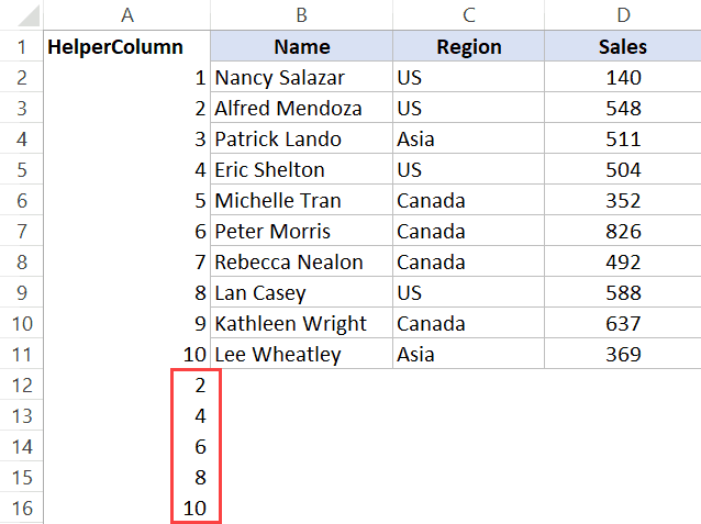
Go to the last filled cell in the helper column and then select the cell below it.
Enter 2 in this cell and 4 in the cell below it. We are using numbers in multiples of 2 as we want one blank row after every two rows.
Select both the cells and place the cursor at the bottom-right of the selection.
When the cursor changes to a plus icon, click and drag it down. This will fill a series of numbers (just as we got in step 3). Make sure you get a number bigger than what you have in the dataset. For example, if there are 10 records in the dataset, make sure you get at least till the number 10.
Select the entire dataset (including all the cells in the helper column).
Click the Data tab
Click on the Sort option
In the Sort dialog box, use the following settings:
- Sort by: Helper
- Sort on: Cell Value
- Order: Smallest to Largest
Click OK. This will give you the final data set as shown below (with a blank row after every second row of the dataset)
Delete the helper column.

Similarly, in case you want to insert a blank row after every third row, use the number 3, 6, 9, and so on in Step 5.

Using a Simple VBA Code

While you need a lot of workarounds to insert alternate blank rows in Excel, with VBA it’s all a piece of cake.

With a simple VBA code, all you need to do is select the dataset in which you want to insert a blank row after every row, and simply run the code (takes a single click).

Below is the VBA code that will insert a blank row after every row in the dataset:

Sub InsertAlternateRows()
'This code will insert a row after every row in the selection
'This code has been created by Sumit Bansal from trumpexcel.com
Dim rng As Range
Dim CountRow As Integer
Dim i As Integer
Set rng = Selection
CountRow = rng.EntireRow.Count

For i = 1 To CountRow
    ActiveCell.Offset(1, 0).EntireRow.Insert
    ActiveCell.Offset(2, 0).Select
Next i

End Sub

The above code counts the total number of rows in the selection and uses a For Next loop to cycle through each row and insert a blank row after each existing row in the dataset.

Here are the steps to place this VBA code in the VB Editor in Excel:

Copy the above code
Go to the Developer tab and click on the Visual Basic option. This will open the VB Editor. You can also use the keyboard shortcut ALT + F11
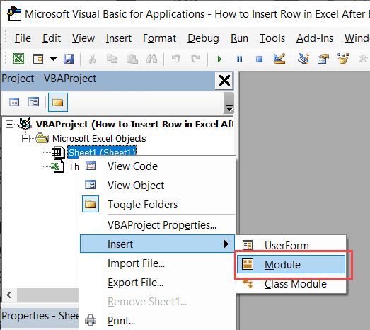
In the VB Editor, right-click on any object in the Project Explorer
Hover the cursor over the Insert option and then click on Module. This will insert a new module
In the Module code window, paste the above code.

Once you have the code in the VB Editor, you can now use this code to insert blank rows after every other row in the dataset.

Here are the steps to use the code to insert blank rows after every row:

Select the entire dataset (except the header row)
Click the Developer tab (in case you don’t have the Developer tab, click here to learn how to get it)
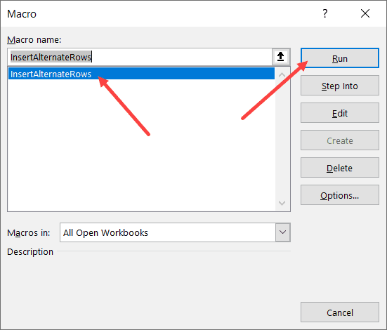
Click on the ‘Macros’ option
In the Macro dialog box, select the macro – ‘InsertAlternateRows’
Click on Run

That’s it!

The above steps would instantly insert alternating blank rows in the dataset.

There are many different ways to run a macro in Excel. For example, if you have to do this quite often, you can add this macro to the Quick Access Toolbar so that you can run it with a single click.

You can read more about different ways to run macros here.

In case you want to insert a blank row after every second row, you can use the below code:

Sub InsertBlankRowAfterEvery2ndRow()
'This code will insert a row after every second row in the selection
'This code has been created by Sumit Bansal from trumpexcel.com
Dim rng As Range
Dim CountRow As Integer
Dim i As Integer
Set rng = Selection
CountRow = rng.EntireRow.Count

For i = 1 To CountRow / 2
    ActiveCell.Offset(2, 0).EntireRow.Insert
    ActiveCell.Offset(3, 0).Select
Next i

End Sub

Hope you found this tutorial useful.

You may also like the following Excel tutorials:

How to Delete Every Other Row in Excel (or Every Nth Row)
Highlight EVERY Other ROW in Excel (using Conditional Formatting)
How to Select Every Third Row in Excel (or select every Nth Row)
Delete Blank Rows in Excel (with and without VBA)
How to Quickly Select Blank Cells in Excel
Hide Zero Values in Excel | Make Cells Blank If the Value is 0
Insert New Columns in Excel

Источник

See Also

Why Do You Need A Blank Value Choice?

Typing Out The List Values

Pulling Values From A Cell Range

I Hope This Helped!

About The Author

Insert a Blank Row After Every Other Row

Using Helper Column and the Sort Feature

Using a Simple VBA Code