Insert new line in excel - Word и Excel - помощь в работе с программами

To start a new line of text or add spacing between lines or paragraphs of text in a worksheet cell, press Alt+Enter to insert a line break.

Double-click the cell in which you want to insert a line break.
Click the location inside the selected cell where you want to break the line.
Press Alt+Enter to insert the line break.

To start a new line of text or add spacing between lines or paragraphs of text in a worksheet cell, press CONTROL + OPTION + RETURN to insert a line break.

Double-click the cell in which you want to insert a line break.
Click the location inside the selected cell where you want to break the line.
Press CONTROL+OPTION+RETURN to insert the line break.

To start a new line of text or add spacing between lines or paragraphs of text in a worksheet cell, press Alt+Enter to insert a line break.

Double-click the cell in which you want to insert a line break (or select the cell and then press F2).
Click the location inside the selected cell where you want to break the line.
Press Alt+Enter to insert the line break.

Double-tap within the cell.
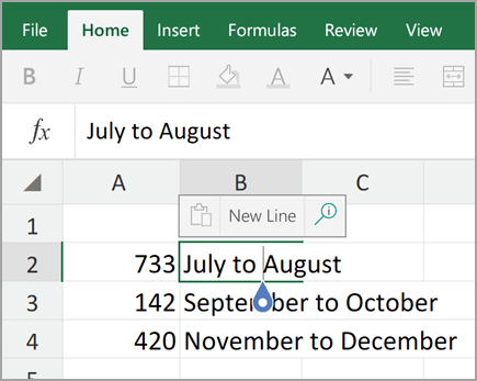
Tap the place where you want a line break, and then tap the blue cursor.
Tap New Line in the contextual menu.

Note: You cannot start a new line of text in Excel for iPhone.

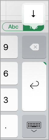
Tap the keyboard toggle button to open the numeric keyboard.
Press and hold the return key to view the line break key, and then drag your finger to that key.

Источник

A new line in excel cell is inserted when one needs to move a string to the next line of the cell. To insert a new line, a line break must be added at the relevant place. A line break tells Excel to break the existing line and begin a new line (within the same cell) with the immediately following character. When line breaks are inserted in a cell, its content can be seen in multiple lines.

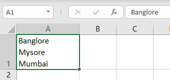
For example, in the following image, a line break has been inserted after the cities Bangalore and Mysore. So, a total of two line breaks have been inserted in cell A1. Notice that the three cities are in three different rows of the same cell.

Starting a new line in an excel cell ensures that the lengthy text strings are split into multiple lines. This improves the readability and lends a neat look to the worksheet. To obtain the right result after inserting line breaks, ensure that the wrap text feature of Excel is turned on.

Insert a New Line in an Excel Cell
- Top 3 Ways to Insert a New Line in a Cell of Excel
  - #1 – Using the Shortcut Keys “Alt+Enter”
  - #2–Using the “CHAR(10)” Formula of Excel
  - #3–Using the Named Formula [CHAR(10)]
- Frequently Asked Questions
- Recommended Articles

Top 3 Ways to Insert a New Line in a Cell of Excel

The methods to start a new line in a cell of Excel are listed as follows:

Shortcut keys “Alt+Enter”
“CHAR(10)” formula of Excel
Named formula [CHAR(10)]

Let us consider an example of each technique.

Note: The line feed (LF) and carriage returnCarriage Return in excel cell is a way to shift to a new line within the same cell. This could be treated as a line breaker which fits in huge data in an organized manner within one cell.read more (CR) are two terms closely related to a line break. The LF moves the cursor to the next line within the cell. In contrast, a CR moves the cursor to the beginning (or the first position) of the same line. So, with a CR alone, the cursor does not move to the next line.

Every operating system considers a line break (LF or CR or a combination of CR and LF) differently. For instance, when a line break is inserted in the Windows operating system, both CR and LF (called CR+LF or CRLF) are inserted together.

The CRLF moves the cursor to the beginning of the next line. However, the “Alt+Enter” method inserts only line feeds in Excel. The ASCII (American Standard Code for Information Interchange) codes for LF and CR are 10 and 13 respectively.

In this article, the usage of code 10 has been shown in example #2. Further, this article uses the term line break in place of line feed and carriage return. Hence, consider all three (line break, line feed, and carriage return) to be the same in this article.

#1 – Using the Shortcut Keys “Alt+Enter”

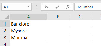
The following image shows the names of three cities of India in cell A1. We want to insert a line break after the first two cities of this cell. Use the keys “Alt+Enter” of Excel.

The steps to insert line breaks by using the keys “Alt+Enter” are listed as follows:

Step 1: Double-click inside cell A1. Next, move and bring the cursor immediately before the “M” of Mysore. To do this, either move the cursor with the arrow keys of the keyboard or click at the stated position with the left-click of the mouse.

The cursor is placed before Mysore because a line break needs to be inserted at this position.

Note: Alternatively, one can also place the cursor at the stated position in the formula bar.

Step 2: Press the keys “Alt+Enter.” For this shortcut to work, hold the “Alt” key while pressing the “Enter” key.

A new line is inserted before “Mysore,” as shown in the following image.

Step 3: Place the cursor before the “M” of Mumbai by using the left-click of the mouse. Press the keys “Alt+Enter,” the way they were pressed in the preceding step.

The name “Mumbai” shifts to a new line within the same cell of Excel. This is shown in the following image.

Step 4: Press the “Enter” key to exit the Edit mode. The following image shows the names of the three cities in multiple lines of a single cell (cell A1) of Excel. This result will be displayed only if the wrap text feature of Excel is turned on.

Notice that the formula bar (in the following image) shows a line break after Bangalore.

Note: The “wrap text” is a toggle button in the “alignment” group of the Home tab. It can also be accessed from the “alignment” tab of the “format cells” window. This window can be opened by pressing the shortcut “Ctrl+1.”

By default, the wrap text feature is turned on when a line break is inserted with the “Alt+Enter” method in Excel. To cross-check, keep cell A1 selected and notice that the “wrap text” button is automatically activated after inserting a line break with the shortcut keys.

If the wrap text button is turned off, the content of cell A1 will display in a single line. However, the line breaks will still be visible in the formula bar.

#2–Using the “CHAR(10)” Formula of Excel

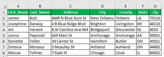
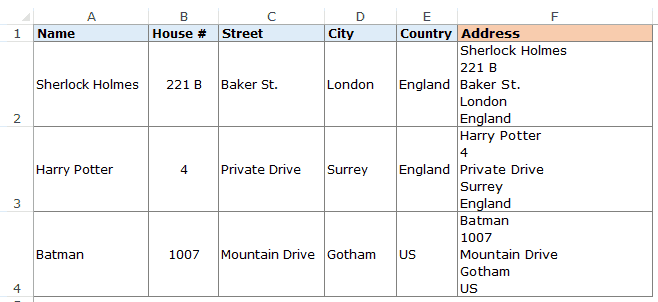
The following image shows the names and addresses of some people. The first and the last names have been split into columns A and B respectively. The address has been split into columns C to G. We want to perform the following tasks:

Join the first and the last name to the full address of each person. For this, combine the strings of columns A and B with those of columns C to G. Use the ampersand (&) to join the stated strings. Ensure that a single space character precedes each string of the address.
Insert a line break between the last name and the first character of the address. Use the CHAR function for inserting line breaks.

In the end, the complete name should be in one line, followed by the address in the subsequent lines of the cell. Further, use a single formula for performing the given tasks. Explain the formula used.

The steps to perform the given tasks by using the ampersand and the CHAR functionThe character function in Excel, also known as the char function, identifies the character based on the number or integer accepted by the computer language. For example, the number for character «A» is 65, so if we use =char(65), we get A.read more are listed as follows:

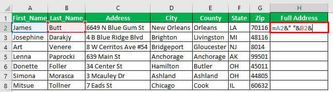
Step 1: Insert a new column to the right of the given dataset. We have inserted column H titled “full address.” This is shown in the following image.

Step 2: Begin by combining the first and last names (of row 2) with the ampersand. To do this, type the following formula in cell H2.

“=A2&“ ”&B2&”

This formula joins the first and the last names of cells A2 and B2 and also inserts a space between them. However, the formula is currently incomplete.

Step 3: Extend the preceding formula to include the CHAR function. Open this function by typing “CHAR,” followed by the opening parenthesis.

The opening of the CHAR function is shown in the following image.

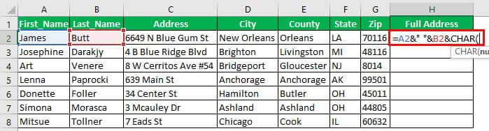
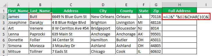
Step 4: Insert the number 10 within the CHAR function. The “CHAR(10)” formula inserts a line break in Excel.

Note: The syntax of the CHAR function is “CHAR(number).” This function returns a character when a number between 1 and 255 is entered. The character is returned from the character set of the user’s computer.

Earlier, the Windows operating system used the ASCII and the ANSI character sets, which have now been replaced by Unicode. The ASCII stands for American Standard Code for Information Interchange. The ANSI character set was created by the American National Standard Institute.

In contrast, the Macintosh operating system uses the Macintosh character set. So, the Macintosh users may use the formula “CHAR(13)” to insert a line break in Excel.

Step 5: Insert the cell references to be joined with the strings of cells A2 and B2. So, in cell H2, enter the following formula by excluding the beginning and ending double quotation marks.

“=A2&” “&B2&CHAR(10)&C2&” “&D2&” “&E2&” “&F2&” “&G2”

Press the “Enter” key. The output appears in cell H2. The formula and the output are shown in the following image. The output is not fully visible as it is in a single line of cell H2 of Excel.

Explanation of the formula: The preceding formula joins the first and the last names (in cells A2 and B2) with the entire address of a person (in cells D2, E2, F2, and G2). The ampersand (&) is used to join.

Notice that, in the formula, a space character has been inserted preceding the strings of cells D2, E2, F2, and G2. This space character is inserted within double quotation marks (like “ ”). These spaces of the formula ensure that spaces are inserted as separators in the output. Moreover, the separators are inserted at exactly those places (in the output) where they have been entered in the formula.

However, no space is inserted between the strings of cells B2 and C2. Rather, the “CHAR(10)” has been used in place of a space. This is because the “CHAR(10)” moves the immediately following string (of cell C2) to the next line.

Step 6: Activate the wrap text feature of Excel to see the entire content of cell H2. So, select cell H2 and click the “wrap text” button in the “alignment” group of the Home tab.

The output is shown in the following image. The full name and the complete address are visible in cell H2. Not only the strings of cells A2 to G2 have been joined, but a line break has also been inserted after the name (James Butt). As a result, a legible output has been obtained in cell H2.

Note: When a line break is inserted by the CHAR function, the wrap text feature of Excel is not turned on by default. Rather, this feature needs to be enabled manually to see the impact of the line break.

Step 7: Drag the formula of cell H2 till cell H8 by using the fill handle. The fill handle is displayed at the bottom-right corner of cell H2.

The dragging of the fill handle and the outputs are shown in the following image. Hence, the names and addresses have been consolidated neatly in column H.

#3–Using the Named Formula [CHAR(10)]

Working on the dataset of example #2, we want to perform the following tasks:

Assign the name “NL” to the “CHAR(10)” formula. By doing this, “CHAR(10)” becomes a named formula.
Add the comment “new line inserter” to the name “NL.”
Show how to use the name “NL” (representing the named formula) in the ampersand and CHAR formula of example #2. Explain the formula thus used.

Use the “define name” property of Excel for the first two bullet points.

The steps to perform the given tasks by using the named formula are listed as follows:

Step 1: Click “define name” from the “defined names” group of the Formulas tab. This option is shown in the following image.

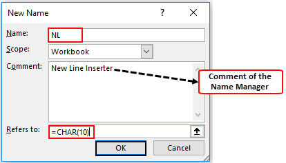
Step 2: The “new name” window opens, as shown in the following image. Make the following insertions in this window:

In the “name” box, enter the name “NL.”
In the “scope” box, let the option “workbook” remain selected.
In the “comment” box, enter the string “new line inserter.”
In the “refers to” box, enter the formula “=CHAR(10).”

Ensure that the insertions of points “a,” “c,” and “d” are entered without the beginning and ending double quotation marks. Click “Ok” once the insertions are done.

Note 1: The name and the comment cannot exceed 255 characters in length. The name must begin with a letter, underscore (_) or backslash (). Further, the name should not consist of any space characters.

Note 2: The “new name” window can also be opened by clicking “name managerThe name manager in Excel is used to create, edit, and delete named ranges. For example, we sometimes use names instead of giving cell references. By using the name manager, we can create a new reference, edit it, or delete it.read more” (in the “defined names” group) from the Formulas tab and then clicking “new” (in the “name manager” window).

Step 3: Use “NL” in place of “CHAR(10)” in the following formula.

“=A2&” “&B2&NL&C2&” “&D2&” “&E2&” “&F2&” “&G2”

Press the “Enter” key. The outputs are shown in the following image.

Note: When the “N” of “NL” is typed in the formula, Excel shows the name (NL) as well as the comment (new line inserter) in a list of suggestions. To select “NL” from this list, just double-click it.

Explanation of the formula: The outputs of the preceding formula are the same as that of example #2 (in step 7). This is because other than the name “NL,” the formulas of the two examples (examples #2 and #3) are the same.

Since “CHAR(10)” has been named “NL,” we have used this name in the formula instead of the CHAR function. The “wrap text” feature has also been applied to cell H2. This is the reason its content has fitted into multiple lines of cell H2 of Excel.

Notice that using a different name for “CHAR(10)” has not impacted the result. Rather, using the name “NL” has made the preceding formula compact and understandable.

Note: In this example, “CHAR(10)” is considered a named formula. A named formula is one that has been assigned a name in Excel. Assigning a name (like “NL”) to a formula [like “CHAR(10)”] helps refer to the formula by its name.

So, every time one needs to use “CHAR(10)” in the formulas of the current workbook, one can use “NL” in its place. This is because the “scope” in the “new name” window has been set as “workbook.”

Frequently Asked Questions

1. What does it mean to insert a new line in a cell of Excel? Suggest the shortcuts for inserting a line break in Windows and Macintosh operating systems.

Inserting a new line means moving the content of a cell to the next line. This allows one to break lengthy text strings and display their data in multiple lines of a single cell. The shortcuts for inserting a line break in Excel are stated as follows:

Windows operating system – The shortcut is “Alt+Enter.” For this shortcut to work, hold the “Alt” key while pressing the “Enter” key.

Macintosh operating system – The shortcut is “Control+Option+Return” (or “Control+Command+Return”). For this shortcut to work, hold the “Control” and the “Option” keys while pressing the “Return” key.

Note: Before using the preceding shortcuts, ensure that the cursor is placed where a line break needs to be inserted.

2. How to use the CONCATENATE function and the Find and Replace feature to insert a new line in Excel?

The CONCATENATE function joins the values of different cells in a single cell. Thereafter, the “CHAR(10)” inserts line breaks in the single output cell.

The CONCATENATE and CHAR formula for inserting a new line in Excel is stated as follows:
“CONCATENATE(cell1,CHAR(10),cell2,CHAR(10),cell3,CHAR(10)…)”

The steps for inserting a new line with the Find and Replace feature of Excel are listed as follows:

a. Select the cells in which a new line needs to be inserted.
b. Press the keys “Ctrl+H” to open the Replace tab of the Find and Replace window. Alternatively, click the “find & select” drop-down from the “editing” group of the Home tab. Then, select the “replace” option.
c. In the “find what” box, type the separator that separates the strings. For instance, if a comma separates the strings, type a comma. Likewise, if a space separates the strings, type a space.
d. In the “replace with” box, press the keys “Ctrl+J.” A small, blinking dot appears in this box.
e. Click “replace all.”

In the selected cells, all occurrences of the separator (typed in step “c”) will be replaced by line breaks.

Note: Use the Find and Replace feature for inserting line breaks when each selected cell contains at least one occurrence of the separator. At the same time, there is a need to replace all these occurrences with line breaks.

3. How to remove a line break from a cell of Excel?

The formula to remove a line break from a cell is stated as follows:
“=SUBSTITUTE(cell1,CHAR(10),””)”

The formula to insert a comma in place of a line break is stated as follows:
“=SUBSTITUTE(cell1,CHAR(10),”,”)”

In both the preceding formulas, “cell1” is the cell that contains the string with line breaks. Further, the SUBSTITUTE function replaces every occurrence of “CHAR(10)” with a blank (“”) or a comma (“,”).

Note: Alternatively, the line breaks can be removed with the Find and Replace feature. Press the keys “Ctrl+J” in the “find what” box. In the “replace with” box, type a separator (like a space or comma) that needs to be inserted in place of a line break. Click “replace all” at the end.

Since removing line breaks with the Find and Replace feature may not always work as desired, one can use the preceding SUBSTITUTE and CHAR formulas.

Start a New Line in Excel Cell – Keyboard Shortcut

To start a new line in an Excel cell, you can use the following keyboard shortcut:

For Windows – ALT + Enter.
For Mac – Control + Option + Enter.

Here are the steps to start a new line in Excel Cell using the shortcut ALT + ENTER:

Double click on the cell where you want to insert the line break (or press F2 key to get into the edit mode).
Place the cursor where you want to insert the line break.
Hold the ALT key and press the Enter key for Windows (for Mac – hold the Control and Option keys and hit the Enter key).

See Also: 200+ Excel Keyboard Shortcuts.

Start a New Line in Excel Cell Using Formula

While keyboard shortcut is fine when you are manually entering data and need a few line breaks.

But in case you need to combine cells and get a line break while combining these cells, you can use a formula to do this.

Using TextJoin Formula

If you’re using Excel 2019 or Office 365 (Windows or Mac), you can use the TEXTJOIN function to combine cells and insert a line break in the resulting data.

For example, suppose we have a dataset as shown below and you want to combine these cells to get the name and the address in the same cell (with each part in a separate line):

The following formula will do this:

=TEXTJOIN(CHAR(10),TRUE,A2:E2)

At first, you may see the result as one single line that combines all the address parts (as shown below).

To make sure you have all the line breaks in between each part, make sure the wrap text feature is enabled.

To enable Wrap text, select the cells with the results, click on the Home tab, and within the alignment group, click on the ‘Wrap Text’ option.

Once you click on the Wrap Text option, you will see the resulting data as shown below (with each address element in a new line):

Note: If you are using MAC, use CHAR(13) instead of CHAR(10).

Using Concatenate Formula

If you’re using Excel 2016 or prior versions, you won’t have the TEXTJOIN formula available.

So you can use the good old CONCATENATE function (or the ampersand & character) to combine cells and get line break in between.

Again, considering you have the dataset as shown below that you want to combine and get a line break in between each cell:

For example, if I combine using the text in these cells using an ampersand (&), I would get something as shown below:

While this combines the text, this is not really the format that I want. You can try using the text wrap, but that wouldn’t work either.

If I am creating a mailing address out of this, I need the text from each cell to be in a new line in the same cell.

To insert a line break in this formula result, we need to use CHAR(10) along with the above formula.

CHAR(10) is a line feed in Windows, which means that it forces anything after it to go to a new line.

So to do this, use the below formula:

=A2&CHAR(10)&B2&CHAR(10)&C2&CHAR(10)&D2&CHAR(10)&E2

This formula would enter a line break in the formula result and you would see something as shown below:

IMPORTANT: For this to work, you need to wrap text in excel cells. To wrap text, go to Home –> Alignment –> Wrap Text. It is a toggle button.

Tip: If you are using MAC, use CHAR(13) instead of CHAR(10).

You may also like the following Excel Tutorial:

Insert Picture in an Excel Cell.
How to Split Multiple Lines in a Cell into a Separate Cells / Columns
Combine Cells in Excel
CONCATENATE Excel Range with and without a separator
MS Help – Start a New Line.
How to Switch Between Sheets in Excel? (7 Better Ways)

Источник

Home / Excel Formulas / How to Add New Line in a Cell in Excel (Line Break)

To start or insert a new line within a cell in Excel, there are multiple ways that you can use. But the easiest one is to use the keyboard shortcut Alt + Enter that you can use while entering values, and apart from that there are ways that you can use it with a formula, like, TEXTJOIN and CONCATENATE.

In this tutorial, we will look at all these methods and you can choose any of these according to your need.

sample-file.xlsx

Steps a Start a New Line in Excel in a Cell (Manually)

In the following example, I want to add my name to cell A1, but I want to add my last name to a new line inside the cell only. So let’s use the following steps for this:

The first thing that you need to do is to edit the cell and enter the first value by normally typing it.
After that, you need to press and hold the ALT key from your keyboard.
Next, you need to press the enter key while pressing and holding the ALT key. This will move your cursor to the new line.
Now, you can enter the last name in the second line, just by typing it.
In the end, hit enter to come out of the edit cell mode.

So here you have a cell where you have a value in the new line (second line) within the cell.

But there is one thing that you need to know when you insert a new line in the cell using the keyboard shortcut, Excel activates the wrap text for that cell automatically.

Now if you remove this wrap text formatting from the cell, this will also remove the new line from the cell that you have added while entering the values.

If you need to insert a new line in multiple cells in a single go, the best way is to use a formula. In the following example, you have first and last names in columns A and B.

Now, you need to CONCATENATE both to get the full name in column C. And here you also need to use the CHAR function to enter a new line within the cell.

First thing is to enter the concatenate function in cell C2.
After that, in the first argument, refer to cell A2 where you have the first name.
Next, in the second argument enter the CHAR function and use 10 as the argument value.
From here, in the third argument, refer to cell B2 where you have the last name.
Now, hit the enter key and apply this formula to all the names that you have in the column.
In the end, to get the line break, you need to apply wrap text to the entire column C.

=CONCATENATE(A2,CHAR(10),B2)

In the same way, you can use the TEXTJOIN as well which also helps you to combine two values from the cell, and then using the CHAR function you can add a new line (line break) within the cell.

=TEXTJOIN(CHAR(10),TRUE,A2:B2)

Once you create a formula using TEXTJOIN and CHAR, you also need to apply the wrap text formatting to the cell, so that it shows both values in two different lines using a line break.

Named Range Trick to Insert a New Line in a Cell

You can also create a named range in Excel and add a CHAR function inside that named range. Go to the Formula Tab ⇢ Name Manager ⇢ New.

Now, if you want to add a new line in a cell while combining two values you can simply use a formula like the one below.

In this method, you also need to apply wrap text to the cell to get the second value in the new line.

Источник

Если вам нужно вставить новую строку в ячейку Excel, как вы можете с этим справиться? В этой статье представлены 4 решения для вас.

Начать новую строку в ячейке с помощью ярлыка
Начать новую строку в ячейке с формулой
Начать новую строку в ячейке с буфером обмена
Начните новые строки в ячейках с помощью классного инструмента

Начать новую строку в ячейке с помощью ярлыка

Вы можете использовать другой + Enter клавиши, чтобы легко начать новую строку в ячейке.

Дважды щелкните ячейку, поместите курсор в то место, где вы начнете новую строку, а затем нажмите другой + Enter ключи вместе. И тогда вы увидите, что в ячейку вставлена новая строка.

Начать новую строку в ячейке с формулой

Вы также можете применить формулу для начала новой строки в ячейке.

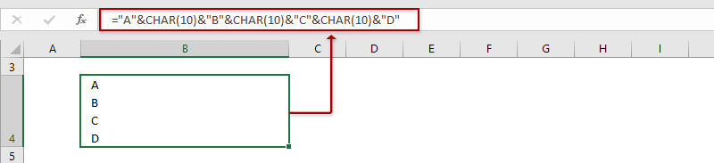
Например, содержимое ячейки — «ABCD», вы можете изменить содержимое на формулу ниже и нажать Enter ключ. Затем включите деформацию текста, нажав Главная > Перенести текст.

= «A» & CHAR (10) & «B» & CHAR (10) & «C» & CHAR (10) & «D»

Начать новую строку в ячейке с буфером обмена

Если вы хотите начинать новые строки для ввода содержимого соседних ячеек, вы можете использовать буфер обмена, чтобы легко это сделать в Excel.

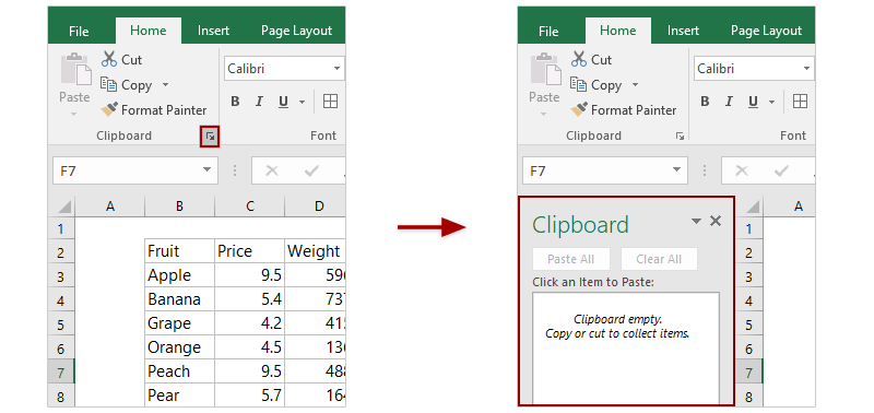
1. Включите буфер обмена, щелкнув привязку в правом нижнем углу буфер обмена группы на Главная меню.

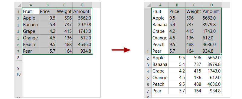
2. Выберите строки, которые вы добавите как новые строки в ячейку, и нажмите Ctrl + C ключи вместе, чтобы скопировать его. Затем диапазон добавляется в буфер обмена.

3. Дважды щелкните ячейку и щелкните скопированный диапазон в буфере обмена.

Затем скопированный диапазон добавляется в эту ячейку, и каждая строка добавляется как новая строка. Смотрите скриншот:

Начните новые строки в ячейках с помощью классного инструмента

Если у вас есть Kutools for Excel установлен, можно применить его круто Сочетать возможность легко добавлять содержимое ячеек в ту же строку или столбец, что и новая строка в ячейках.

Kutools for Excel— Включает более 300 удобных инструментов для Excel. Полнофункциональная бесплатная 60-дневная пробная версия, кредитная карта не требуется! Get It Now

1. Выберите нужный диапазон и нажмите Кутулс > Сочетать.

2. В диалоговом окне «Объединить столбцы или строки» установите флажок Объединить ряды и New Line параметры и щелкните Ok кнопка. Смотрите скриншот:

Теперь вы увидите, что содержимое ячейки в каждом столбце добавляется в виде новых строк в первую ячейку соответствующего столбца. Смотрите скриншот:

Если проверить Объединить столбцы и New Line параметры и щелкните Ok в диалоговом окне «Объединить столбцы или строки», вы увидите, что содержимое ячеек каждой строки вставляется как новые строки в первую ячейку соответствующей строки. Смотрите скриншот:

Статьи по теме:

Лучшие инструменты для работы в офисе

Kutools for Excel Решит большинство ваших проблем и повысит вашу производительность на 80%

Снова использовать: Быстро вставить сложные формулы, диаграммы и все, что вы использовали раньше; Зашифровать ячейки с паролем; Создать список рассылки и отправлять электронные письма …
Бар Супер Формулы (легко редактировать несколько строк текста и формул); Макет для чтения (легко читать и редактировать большое количество ячеек); Вставить в отфильтрованный диапазон…
Объединить ячейки / строки / столбцы без потери данных; Разделить содержимое ячеек; Объединить повторяющиеся строки / столбцы… Предотвращение дублирования ячеек; Сравнить диапазоны…
Выберите Дубликат или Уникальный Ряды; Выбрать пустые строки (все ячейки пустые); Супер находка и нечеткая находка во многих рабочих тетрадях; Случайный выбор …
Точная копия Несколько ячеек без изменения ссылки на формулу; Автоматическое создание ссылок на несколько листов; Вставить пули, Флажки и многое другое …
Извлечь текст, Добавить текст, Удалить по позиции, Удалить пробел; Создание и печать промежуточных итогов по страницам; Преобразование содержимого ячеек в комментарии…
Суперфильтр (сохранять и применять схемы фильтров к другим листам); Расширенная сортировка по месяцам / неделям / дням, периодичности и др .; Специальный фильтр жирным, курсивом …
Комбинируйте книги и рабочие листы; Объединить таблицы на основе ключевых столбцов; Разделить данные на несколько листов; Пакетное преобразование xls, xlsx и PDF…
Более 300 мощных функций. Поддерживает Office/Excel 2007-2021 и 365. Поддерживает все языки. Простое развертывание на вашем предприятии или в организации. Полнофункциональная 30-дневная бесплатная пробная версия. 60-дневная гарантия возврата денег.

Вкладка Office: интерфейс с вкладками в Office и упрощение работы

Включение редактирования и чтения с вкладками в Word, Excel, PowerPoint, Издатель, доступ, Visio и проект.
Открывайте и создавайте несколько документов на новых вкладках одного окна, а не в новых окнах.
Повышает вашу продуктивность на 50% и сокращает количество щелчков мышью на сотни каждый день!

Комментарии (0)

Оценок пока нет. Оцените первым!

Источник

Table of contents

Top 3 Ways to Insert a New Line in a Cell of Excel

#1 – Using the Shortcut Keys “Alt+Enter”

#2–Using the “CHAR(10)” Formula of Excel

#3–Using the Named Formula [CHAR(10)]

Frequently Asked Questions

Recommended Articles

Start a New Line in Excel Cell – Keyboard Shortcut

Start a New Line in Excel Cell Using Formula

Using TextJoin Formula

Using Concatenate Formula

Steps a Start a New Line in Excel in a Cell (Manually)

Named Range Trick to Insert a New Line in a Cell

Начать новую строку в ячейке с помощью ярлыка

Начать новую строку в ячейке с формулой

Начать новую строку в ячейке с буфером обмена

Начните новые строки в ячейках с помощью классного инструмента

Статьи по теме:

Лучшие инструменты для работы в офисе

Kutools for Excel Решит большинство ваших проблем и повысит вашу производительность на 80%

Вкладка Office: интерфейс с вкладками в Office и упрощение работы