
Insert or delete rows and columns
Insert and delete rows and columns to organize your worksheet better.

Note: Microsoft Excel has the following column and row limits: 16,384 columns wide by 1,048,576 rows tall.
Insert or delete a column
-
Select any cell within the column, then go to Home > Insert > Insert Sheet Columns or Delete Sheet Columns.
-
Alternatively, right-click the top of the column, and then select Insert or Delete.
Insert or delete a row
-
Select any cell within the row, then go to Home > Insert > Insert Sheet Rows or Delete Sheet Rows.
-
Alternatively, right-click the row number, and then select Insert or Delete.
Formatting options
When you select a row or column that has formatting applied, that formatting will be transferred to a new row or column that you insert. If you don’t want the formatting to be applied, you can select the Insert Options button after you insert, and choose from one of the options as follows:
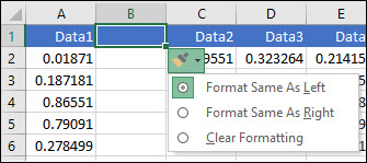
If the Insert Options button isn’t visible, then go to File > Options > Advanced > in the Cut, copy and paste group, check the Show Insert Options buttons option.
Insert rows
To insert a single row: Right-click the whole row above which you want to insert the new row, and then select Insert Rows.
To insert multiple rows: Select the same number of rows above which you want to add new ones. Right-click the selection, and then select Insert Rows.
Insert columns
To insert a single column: Right-click the whole column to the right of where you want to add the new column, and then select Insert Columns.
To insert multiple columns: Select the same number of columns to the right of where you want to add new ones. Right-click the selection, and then select Insert Columns.
Delete cells, rows, or columns
If you don’t need any of the existing cells, rows or columns, here’s how to delete them:
-
Select the cells, rows, or columns that you want to delete.
-
Right-click, and then select the appropriate delete option, for example, Delete Cells & Shift Up, Delete Cells & Shift Left, Delete Rows, or Delete Columns.
When you delete rows or columns, other rows or columns automatically shift up or to the left.
Tip: If you change your mind right after you deleted a cell, row, or column, just press Ctrl+Z to restore it.
Insert cells
To insert a single cell:
-
Right-click the cell above which you want to insert a new cell.
-
Select Insert, and then select Cells & Shift Down.
To insert multiple cells:
-
Select the same number of cells above which you want to add the new ones.
-
Right-click the selection, and then select Insert > Cells & Shift Down.
Need more help?
You can always ask an expert in the Excel Tech Community or get support in the Answers community.
See Also
Basic tasks in Excel
Overview of formulas in Excel
Need more help?
Want more options?
Explore subscription benefits, browse training courses, learn how to secure your device, and more.
Communities help you ask and answer questions, give feedback, and hear from experts with rich knowledge.
Creating new tables, reports and pricelists of different types, we cannot predict the number of necessary rows and columns. Using Excel program implies to a great extent creating and setting up spreadsheets, which requires inserting and deleting different elements.
First, let’s consider the methods of inserting sheet rows and columns when creating spreadsheets.
Note that in this tutorial we indicate hot keys for adding or deleting rows and columns. They should be used after highlighting the whole row or column. To highlight the row where the cursor is placed, press the combination of hot keys: SHIFT+SPACEBAR. Hot keys for highlighting a column are CTRL+SPACEBAR.
How to insert a column between other columns?
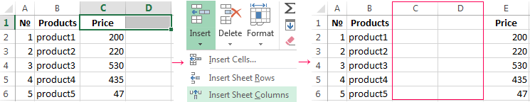
Assuming you have a pricelist lacking line item numbering:
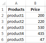
To insert a column between other columns for filling in pricelist items numbering you can use one of the two ways:
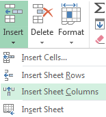
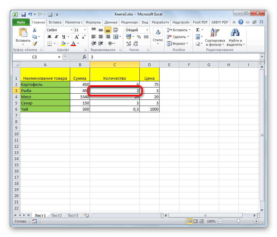
- Move the cursor to activate A1 cell. Then go to tab «HOME», tool section «Cells» and click «Insert», in the popup menu select «Insert Sheet Columns» option.
- Right-click the heading of column A. Select «Insert» option on the shortcut menu.
- Select the column, and press the hotkey combination CTRL+SHIFT+PLUS.
Now you can type the numbers of pricelist line items.
Simultaneous insertion of several columns
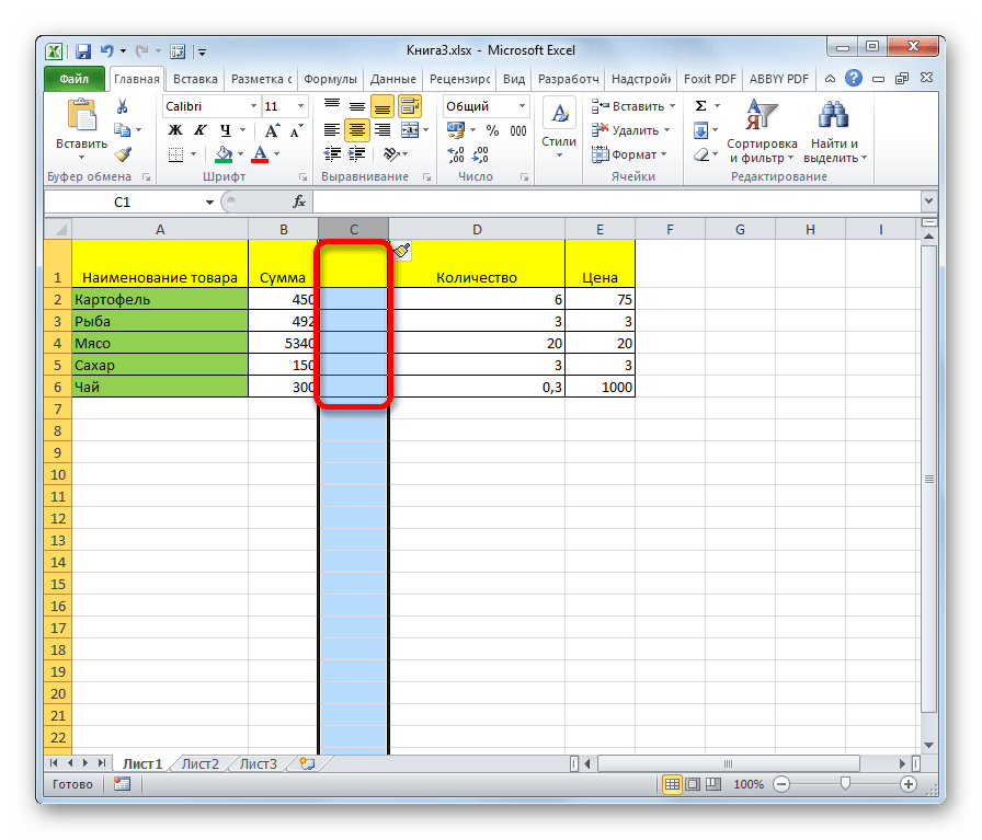
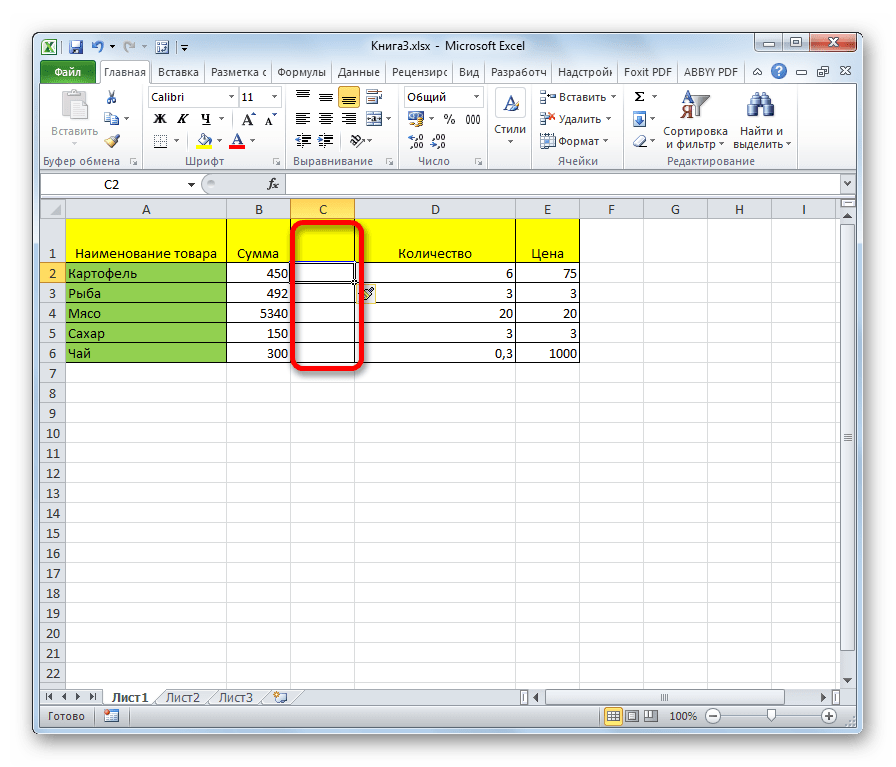
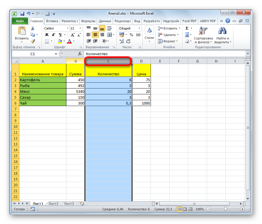
The pricelist still lacks two columns: quantity and units (items, kilograms, liters, packs). To add simultaneously, highlight the two-cell range (C1:D1). Then use the same tool on the «Insert»-«Insert Sheet Columns» main tab.
Alternatively, highlight two headings of columns C and D, right-click and select «Insert» option.
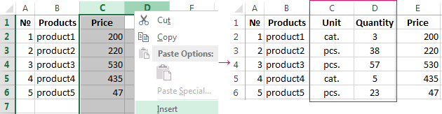
Note. Columns are always added to the left side. There appear as many new columns as many old ones have been highlighted. The order of inserted also depends on the order of highlighting. For example, next but one etc.
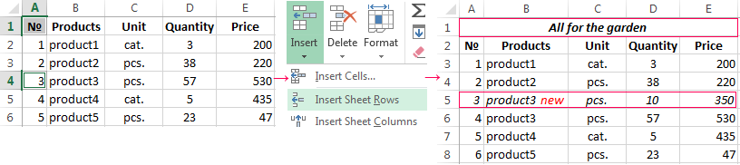
How to insert a row between rows in Excel?
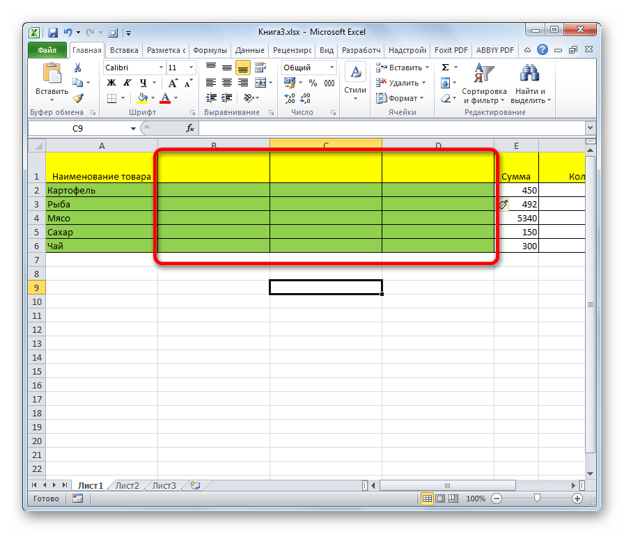
Now let’s add a heading and a new goods line item «All for the garden» to the pricelist. To this end, let’s insert two new rows simultaneously.
Highlight the nonadjacent range of two cells A1,A4 (note that character “,” is used instead of character “:” – it means that two nonadjacent ranges should be highlighted; to make sure, type A1; A4 in the name field and press Enter). You know from the previous tutorials how to highlight nonadjacent ranges.
Now once again use the tool «HOME»-«Insert»-«Insert Sheet Columns». The picture shows how to insert a blank row between other rows in Excel.
It is easy to guess the second way. You need to highlight headings of rows 1 and 3, right-click on one of the highlighted rows and select «Insert» option.
To add a row or a column in Excel use hot keys CTRL+SHIFT+PLUS having highlighted the appropriate row or column.
Note. New rows are always added above the highlighted rows.
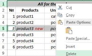
Deleting rows and columns
When working with Excel you need to delete rows and columns as often as to insert them. Therefore, you have to practice.
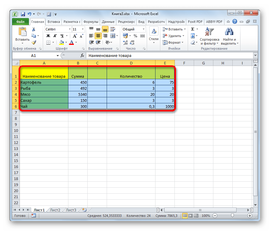
By way of illustration, let’s delete from our pricelist the numbering of goods line items and the unit column simultaneously.
Highlight the nonadjacent range of cells A1; D1 and select «HOME»-«Delete»-«Delete Sheet Rows». The shortcut menu can also be used for deleting if you highlight headings A1 and D1 instead of cells.
Row deleting is performed in the similar way. You only need to select a tool in the appropriate menu. Applying a shortcut menu is the same. You only have to highlight the rows correspondingly by row numbers.
To delete a row or a column in Excel, use hot keys CTRL+MINUS having preliminary highlighted them.
Note. Inserting new columns and rows is in fact substitution, as the number of rows (1 048 576) and columns (16 384) doesn’t change. The new just replace the old ones. You should consider this fact when filling in the sheet with data by more than 50% — 80%.
Adding or removing columns in Excel in a common task when you’re working with data in Excel.
And just like every other thing in Excel, there are multiple ways to insert columns as well. You can insert one or more single columns (to the right/left of a selected one), multiple columns (adjacent or non-adjacent), or a column after every other column in a dataset.
Each of these situations would need a different method to insert a column.
Note: All the methods shown in this tutorial will also work in case you want to insert new rows
Insert New Columns in Excel
In this tutorial, I will cover the following methods/scenarios to insert new columns in Excel:
- Insert one new column (using keyboard shortcut or options in the ribbon)
- Add multiple new columns
- Add non-adjacent columns at one go
- Insert new columns after every other column
- Insert a New Column in an Excel Table
Insert a New Column (Keyboard Shortcut)
Suppose you have a dataset as shown below and you want to add a new column to the left of column B.
Below is the keyboard shortcut to insert a column in Excel:
Control Shift + (hold the Control and Shift keys and press the plus key)
Command + I if you’re using Mac
Below are the steps to use this keyboard shortcut to add a column to the left of the selected column:
- Select a cell in the column to the left of which you want to add a new column
- Use the keyboard shortcut Control Shift +
- In the Insert dialog box that opens, click the Entire Column option (or hit the C key)

- Click OK (or hit the Enter key).

The above steps would instantly add a new column to the left of the selected column.
Another way to add a new column is to first select an entire column and then use the above steps. When you select an entire column, using the Control Shift + shortcut will not show the insert dialog box.
It will just add the new column right away.
Below is the keyboard shortcut to select the entire column (once you select a cell in the column):
Control + Spacebar (hold the Control key and press the space bar key)
Once you have the column selected, you can use Control Shift + to add a new column.
If you’re not a fan of keyboard shortcuts, you can also use the right-click method to insert a new column. Simply right-click on any cell in a column, right-click and then click on Insert. This will open the Insert dialog box where you can select ‘Entire Column’.

This would insert a column to the left of the column where you selected the cell.
Add Multiple New Columns (Adjacent)
In case you need to insert multiple adjacent columns, you can either insert one column and time and just repeat the same process (you can use the F4 key to repeat the last action), or you can insert all these columns at one go.
Suppose you have a dataset as shown below and you want to add two columns to the left of column B.
Below are the steps to do this:
- Select two columns (starting with the one on the left of which you want to insert the columns)
- Right-click anywhere in the selection
- Click on Insert

The above steps would instantly insert two columns to the left of Column B.
In case you want to insert any other number of columns (say 3 or 4 or 5 columns), you select that many to begin with.
Add Multiple New Columns (Non-Adjacent)
The above example is quick and fast when you want to add new adjacent columns (i.e., a block of 3 adjacent columns as shown above).
But what if you want to insert columns but these are non-adjacent.
For example, suppose you have a dataset as shown below, and you want to insert one column before Column B and one before Column D.

While you can choose to do this one by one, there is a better way.
Below are the steps to add multiple non-adjacent columns in Excel:
- Select the columns where you want to insert a new column.
- Right-click anywhere in the selection
- Click on Insert.

The above steps would instantly insert a column to the left of the selected columns.

Insert New Columns After Every Other Column (Using VBA)
Sometimes, you may want to add a new column after every other column in your existing dataset.
While you can do this manually, if you’re working with a large dataset, this can take some time.
The faster way of doing this would be to use a simple VBA code to simply insert a column after every column in your dataset.
Sub InsertColumn()
'Code created by Sumit Bansal from trumpexcel.com

Dim ColCount As Integer
Dim i As Integer

StartCol = Selection.Columns.Count + Selection.Columns(1).Column
EndCol = Selection.Columns(1).Column

For i = StartCol To EndCol Step -1
    Cells(1, i).EntireColumn.Insert
Next i

End Sub
The above code will go through each column in the selection and insert a column to the right of the selected columns.
You can add this code to a regular module and then run this macro from there.
Or, if you have to use this functionality regularly, you can also consider adding it to Personal Macro Workbook and then adding it to the Quick Access Toolbar. This way, you will always have access to this code and can run it with a single click.
Note: The above code also works when you have the data formatted as an Excel table.
Add a Column in an Excel Table
When you convert a dataset into an Excel Table, you lose some of the flexibility that you have with regular data when it comes to inserting columns.
For example, you can not select non-contiguous columns and insert columns next to it at one go. You will have to do this one by one.
Suppose you have an Excel Table as shown below.
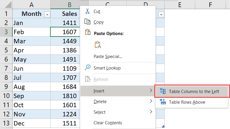
To insert a column to the left of column B, select any cell in the column, right-click, go to the Insert option and click on ‘Table Columns to the left’.
This will insert a column to the left of the selected cell.
In case you select a cell in Column B and one in Column D, you will notice that the ‘Table Columns to the left’ option is grayed out. In this case, you will have to insert columns one by one only.
What’s surprising is that this works when you select non-contiguous rows, but not with columns.
So these are some of the methods you can use to insert new columns in Excel. All the methods covered in this tutorial will also work if you want to insert new rows (the VBA code would need some modification though).
Hope you found this tutorial useful!
You may also like the following Excel tutorials:
- How to Sum a Column in Excel
- How to Unhide COLUMNS in Excel
- How to Move Rows and Columns in Excel
- How to Compare Two Columns in Excel (for matches & differences)
- How to Freeze Multiple Columns in Excel?
Adding a column in Excel means inserting a new column to the existing dataset. Besides inserting, one may need to delete, hide, unhide, and move rows or columns. Such modifications help in structuring and organizing the dataset. As a result, it is essential to be aware of the techniques related to these alterations.
For example, while preparing a consolidated balance sheet, Mr. X realizes that the data related to the previous year is missing. To include this data, he wants to insert a new column. Here, the method of inserting a column comes into use.
Excel provides different ways of performing actions on a dataset. This article discusses the most appropriate and effective methods of working with data. It covers the following aspects: –
- Insert Excel columns (alternate methods and shortcuts)
- Delete columns and rows
- Hide and unhide rows or columns
- Move rows or columns
Apart from inserting columns in Excel, the remaining topics have been covered in brief.
Table of contents
- How to Add/Insert Columns in Excel?
- Example #1–Add Columns in Excel
- Example #2–Alternate Method to Insert Rows and Columns in Excel
- Example #3–Hide and Unhide Columns & Rows in Excel
- Example #4–Move Rows or Columns in Excel
- Shortcuts to Insert Columns in Excel
- Frequently Asked Questions
- Recommended Articles
How to Add/Insert Columns in Excel?
Below are some examples through which you may learn how to add and insert columns in Excel.
Example #1–Add Columns in Excel
The following table shows the first and the last names in columns A and B, respectively. We want to insert a new column (column B) between these names, which will display the middle name.

The steps to insert a new column (column B) between two existing columns (columns A and B) are listed as follows:
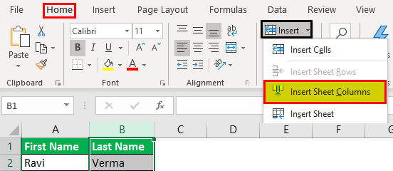
Step 1: Select any cell of column B. Alternatively, one can also select column B, as shown in the following image. Further, click the “Insert” drop-down from the “Home” tab of the Excel ribbonThe ribbon is an element of the UI (User Interface) which is seen as a strip that consists of buttons or tabs; it is available at the top of the excel sheet. This option was first introduced in the Microsoft Excel 2007.read more. Finally, select “Insert Sheet Columns.”
Note: To select a column, click its label or header on top.
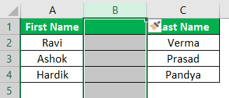
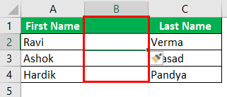
Step 2: A new column (column B) is inserted between the columns containing the first and the last names. As a result, the data (last name) of the previous column B (shown in step 1) now shifts to column C.
Note: Excel inserts a column immediately preceding the column of the selected cell. Hence, one must always choose a cell accordingly. If a column is selected, Excel inserts a column preceding it.
Example #2–Alternate Method to Insert Rows and Columns in Excel
Working on the data of example #1, we need to insert a middle name column using the following methods:
a) Select and right-click a cell
b) Select and right-click a column
a) The steps for inserting a column after selecting and right-clicking a cell are listed as follows:
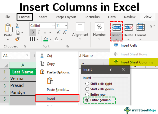
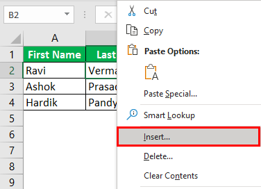
Step 1: Select any cell of column B. This is because a column preceding column B is to be inserted. Right-click the selection and choose “insert,” as shown in the following image.
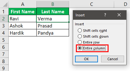
Step 2: The “Insert” dialog box appears. Select “Entire column” to insert a new column.
Note: For inserting a new row, select “Entire row.”
Step 3: A new column (column B) for typing middle names has been inserted.
b) The steps for inserting a column after selecting and right-clicking a column are listed as follows:
Step 1: Select the entire column B. That is because a column preceding column B is to be inserted. Right-click the selection and choose “Insert,” as shown in the following image.
Step 2: A new column B is inserted. The same has been shown under step 3 of method a.
Note: Select the entire row preceding which a new row is inserted for inserting rows. Right-click the selection and choose “Insert.” The same is shown in the following image.

Example #3–Hide and Unhide Columns & Rows in Excel
Working on the data of example #1, we want to perform the following tasks:
a) Hide columns A and B or rows 3 and 4 by right-clicking
b) Hide column A by using the “format” drop-down
c) Unhide columns B and C by right-clicking
a) The steps to hide the columns A and B or rows 3 and 4 by right-clicking are listed as follows:
Step 1: Select columns A and B. Right-click the selection and choose “hide,” as shown in the next image.
Note 1: To select a row or column, click the row number (to the left) or the column label (on top).
Note 2: Multiple adjacent rows or columns can be selected by dragging across the row and column headings. Alternatively, hold the “Shift” key while selecting the rows or columns.
Note 3: We can select non-adjacent rows or columns by holding the “Ctrl” key while making the selections.
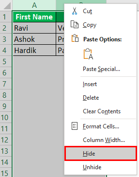
Step 2: Columns A and B will be hidden. Likewise, select rows 3 and 4. Right-click the selection and choose the “Hide” option from the context menu. The same is shown in the following image.
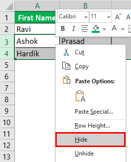
It will hide rows 3 and 4.
b) The steps to hide column A by using the “format” drop-down are listed as follows:
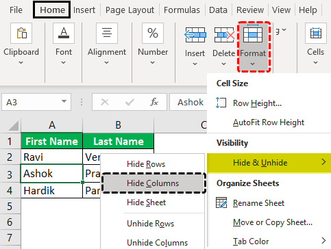
Step 1: Select any cell of column A. Click the “Format” drop-down under the “Home” tab of the Excel ribbon. Next, select “Hide Columns” under the “Hide & Unhide” option.
The same is shown in the following image.
Note: Alternatively, select the relevant column to be hidden. Click “Hide columns” under the “Hide & Unhide” option.
Step 2: We will hide the column of the selected cell, column A. Likewise, to hide rows, select the relevant row. Then, choose “Hide Rows” from the “Hide & Unhide” option of the “Format” drop-down.
c) The steps to unhide columns B and C by right-clicking are listed as follows:
Step 1: Select the unhidden columns (A and D) immediately before and after the hidden columns (B and C). Right-click the selection and choose “Unhide.”
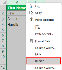
Step 2: The columns B and C will be unhidden. The dataset appears as shown in step 1 of task b.
Likewise, unhide rows by selecting the “Unhide rows” (immediately before and after the hidden rows) and clicking “Unhide” from the context menu.
Example #4–Move Rows or Columns in Excel
Working on the data of example #1, we want to move column B (last name) to precede column A (first name).
The steps to move column B are listed as follows:
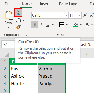
Step 1: Select column B, which is to be moved. Cut it in either of the following ways:
- Press “Ctrl+X.”
- Click the scissors icon from the “Clipboard” group of the “Home” tab.
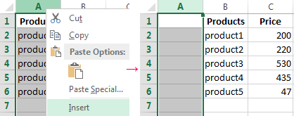
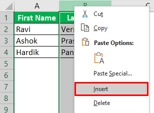
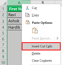
Step 2: Select column A, where the data of column B is to be pasted. Right-click the selection and choose “Insert Cut Cells.”
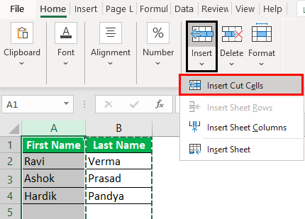
Alternatively, select “Insert Cut Cells” from the “Insert” drop-down of the “Home” tab. The same is shown in the following image.
Note: The “Insert Cut Cells” option will be visible once the selected cells have been cut.
Step 3: The data of column B is pasted into column A. Hence, the first column (column A) now contains the last names. The data of the initial column A (first name) automatically shifts to column B.
The same is shown in the following image.
Note: A row can be selected, cut, and pasted to the desired location. Select the “Insert Cut Cells” option from the “Insert” drop-down of the “Home” tab for pasting.

Shortcuts to Insert Columns in Excel
Let us go through the two shortcuts for inserting columns and rows.
a) Shortcut for inserting with the “Insert” drop-down of the “Home” tab
The excel shortcutAn Excel shortcut is a technique of performing a manual task in a quicker way.read more for inserting a row or column with the “Insert” drop-down works as follows:
- Select a cell preceding which a row or column is inserted.
- Click the “Insert” drop-down from the “Cells” group of the “Home” tab.
- Press “R” to insert a row or “C” to insert a column
A new row or column is inserted depending on the third pointer’s key.
Note: Under the “Insert” drop-down, the “R” of “insert sheet rows” and the “C” of “insert sheet columns” are underlined. Hence, these keys work as shortcuts for inserting rows and columns.
b) Shortcut for inserting with right-click
- The shortcut for inserting a row or column with right-click works as follows:
- Select a cell preceding which a row or column is inserted.
- Right-click the selection and press “I.” The “Insert” dialog box opens.
- Press “R” to insert a row or “C” to insert a column.
- Press the “Enter” key.
A new row or column is inserted depending on the third pointer’s key.
Note: If the “Insert” dialog box does not open in step 2, press the “Enter” key after pressing “I.” It opens the “Insert” dialog box.
Frequently Asked Questions
1. What does it mean to insert a column? How is it done in Excel?
Inserting a column refers to adding a new column to an existing dataset. This new column may contain additional data that can be important for the end-user.
Additionally, there is a possibility that a column has been omitted by mistake. In such cases, inserting a column will be helpful.
The steps to insert a column in Excel are listed as follows:
a. Select the column preceding which a new column is to be inserted.
b. Right-click the selection and choose “Insert” from the context menu.
It will insert the new column immediately before the selected column.
Note: To select a column, click its header (label) on top.
2. How to insert a column in Excel by using a shortcut?
Let us insert a new column E in Excel. The steps to insert a column (column E) by using a shortcut are listed as follows:
a. Select the existing column E.
b. Press the keys “Ctrl+Shift+plus sign(+)” together to insert a column.
It will insert the new column E. The data of the initial column E now shifts to column F.
Note 1: One must select a column carefully. That is because Excel inserts a column preceding the selected column.
Note 2: As an alternative to step a, one can select any cell of column E. After that, press “Ctrl+space” to select the entire column E.
3. How to insert multiple adjacent columns in Excel?
Let us insert columns D, E, and F in Excel. The steps to insert multiple columns (D, E, and F) are listed as follows:
a. Select as many columns in the existing dataset as the number of the new columns to be inserted. So, select the current columns D, E, and F.
b. Press the keys “Ctrl+Shift+plus sign(+)” together.
It will insert the blank columns D, E, and F. The initial columns D, E, and F data shift to columns G, H, and I.
Note 1: Alternative to step a: select adjacent cells of columns D, E, and F. These cells should be in one row. Further, press “Ctrl+space.” As a result, columns D, E, and F will be selected.
Note 2: To select multiple adjacent columns (in step a), drag across the column headings. Alternatively, hold the “Shift” key while selecting the columns.
Note 3: Alternative to step b: right-click the selection and choose “Insert.”
Recommended Articles
This article is a guide to Add Columns in Excel. We also discuss inserting, hiding, and moving rows and columns in Excel and practical examples. You may learn more about Excel from the following articles: –
- Compare Two Columns in Excel for Matches
- 3 Ways to Show Excel Negative Numbers
- Rows vs. Columns
- Move Columns in Excel
Содержание
- Вставка столбца
- Способ 1: вставка через панель координат
- Способ 2: добавление через контекстное меню ячейки
- Способ 3: кнопка на ленте
- Способ 4: применение горячих клавиш
- Способ 5: вставка нескольких столбцов
- Способ 6: добавление столбца в конце таблицы
- Вопросы и ответы

Для работы в Microsoft Excel первоочередной задачей является научиться вставлять строки и столбцы в таблицу. Без этого умения практически невозможно работать с табличными данными. Давайте разберемся, как добавить колонку в Экселе.
Урок: Как добавить столбец в таблицу Microsoft Word
Вставка столбца
В Экселе существует несколько способов вставить столбец на лист. Большинство из них довольно просты, но начинающий пользователь может не сразу со всеми разобраться. Кроме того, существует вариант автоматического добавления строк справа от таблицы.
Способ 1: вставка через панель координат
Одним из самых простых способов вставки является операция через горизонтальную панель координат Excel.
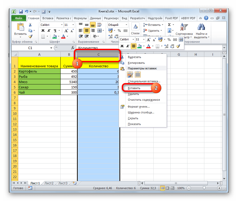
- Кликаем в горизонтальной панели координат с наименованиями колонок по тому сектору, слева от которого нужно вставить столбец. При этом колонка полностью выделяется. Кликаем правой кнопкой мыши. В появившемся меню выбираем пункт «Вставить».
- После этого слева от выделенной области тут же добавляется новый столбец.
Способ 2: добавление через контекстное меню ячейки
Можно выполнить данную задачу и несколько по-другому, а именно через контекстное меню ячейки.
- Кликаем по любой ячейке, находящейся в столбце справа от планируемой к добавлению колонки. Кликаем по этому элементу правой кнопкой мыши. В появившемся контекстном меню выбираем пункт «Вставить…».
- На этот раз добавление не происходит автоматически. Открывается небольшое окошко, в котором нужно указать, что именно пользователь собирается вставить:
- Столбец;
- Строку;
- Ячейку со сдвигом вниз;
- Ячейку со сдвигом вправо.
Переставляем переключатель в позицию «Столбец» и жмем на кнопку «OK».
- После этих действий колонка будет добавлена.


Способ 3: кнопка на ленте
Вставку столбцов можно производить, используя специальную кнопку на ленте.
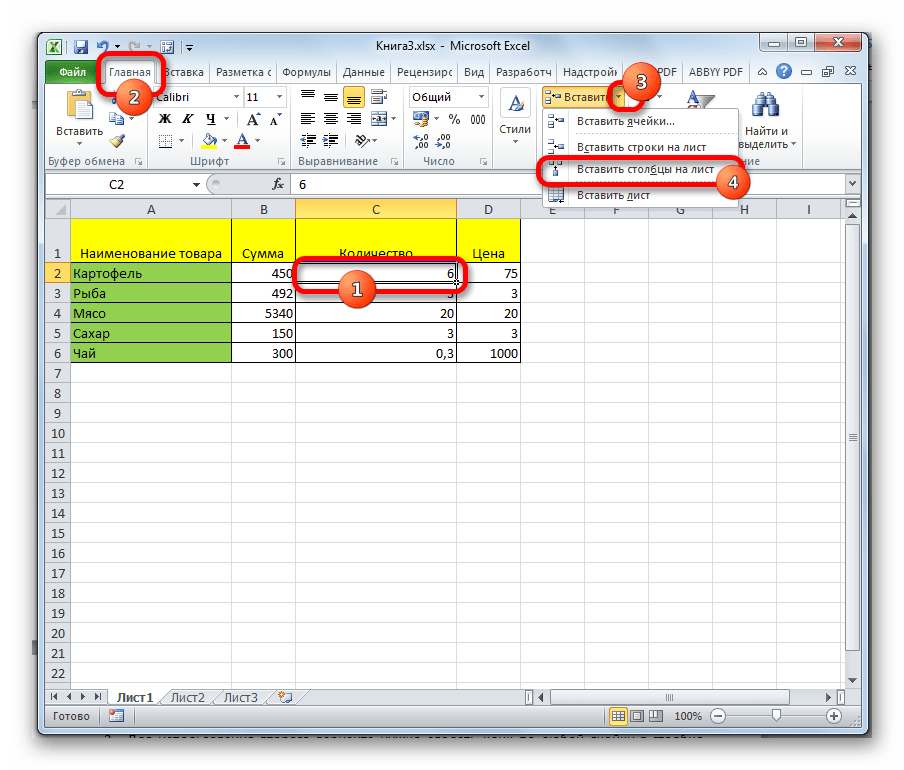
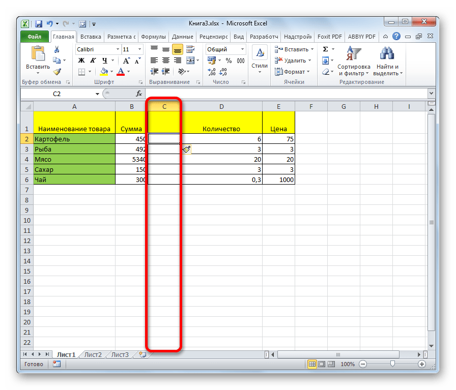
- Выделяем ячейку, слева от которой планируется добавить столбец. Находясь во вкладке «Главная», кликаем по пиктограмме в виде перевернутого треугольника, расположенного около кнопки «Вставить» в блоке инструментов «Ячейки» на ленте. В открывшемся меню выбираем пункт «Вставить столбцы на лист».
- После этого колонка будет добавлена слева от выделенного элемента.
Способ 4: применение горячих клавиш
Также новую колонку можно добавить с помощью горячих клавиш. Причем существует два варианта добавления

- Один из них похож на первый способ вставки. Нужно кликнуть по сектору на горизонтальной панели координат, расположенному справа от предполагаемой области вставки и набрать комбинацию клавиш Ctrl++.
- Для использования второго варианта нужно сделать клик по любой ячейке в столбце справа от области вставки. Затем набрать на клавиатуре Ctrl++. После этого появится то небольшое окошко с выбором типа вставки, которое было описано во втором способе выполнения операции. Дальнейшие действия в точности такие же: выбираем пункт «Столбец» и жмем на кнопку «OK».
Урок: Горячие клавиши в Экселе
Способ 5: вставка нескольких столбцов
Если требуется сразу вставить несколько столбцов, то в Экселе не нужно для этого проводить отдельную операцию для каждого элемента, так как можно данную процедуру объединить в одно действие.
- Нужно сначала выделить столько ячеек в горизонтальном ряду или секторов на панели координат, сколько столбцов нужно добавить.
- Затем применить одно из действий через контекстное меню или при помощи горячих клавиш, которые были описаны в предыдущих способах. Соответствующее количество колонок будет добавлено слева от выделенной области.

Способ 6: добавление столбца в конце таблицы
Все вышеописанные способы подходят для добавления колонок в начале и в середине таблицы. Их можно использовать и для вставки столбцов в конце таблицы, но в этом случае придется произвести соответствующее форматирование. Но существуют пути добавить колонку в конец таблицы, чтобы она сразу воспринималась программой её непосредственной частью. Для этого нужно сделать, так называемую «умную» таблицу.
- Выделяем табличный диапазон, который хотим превратить в «умную» таблицу.
- Находясь во вкладке «Главная», кликаем по кнопке «Форматировать как таблицу», которая расположена в блоке инструментов «Стили» на ленте. В раскрывшемся списке выбираем один из большого перечня стилей оформления таблицы на свое усмотрение.
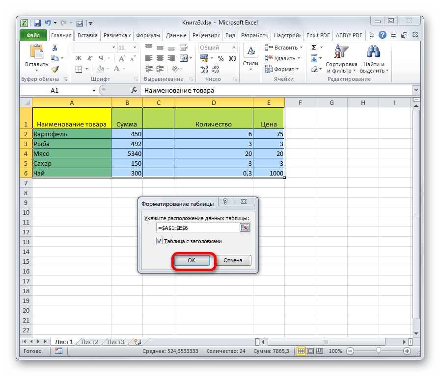
- После этого открывается окошко, в котором отображаются координаты выделенной области. Если вы что-то выделили неправильно, то прямо тут можно произвести редактирование. Главное, что нужно сделать на данном шаге – это проверить установлена ли галочка около параметра «Таблица с заголовками». Если у вашей таблицы есть шапка (а в большинстве случаев так и есть), но галочка у этого пункта отсутствует, то нужно установить её. Если же все настройки выставлены правильно, то просто жмем на кнопку «OK».
- После данных действий выделенный диапазон был отформатирован как таблица.
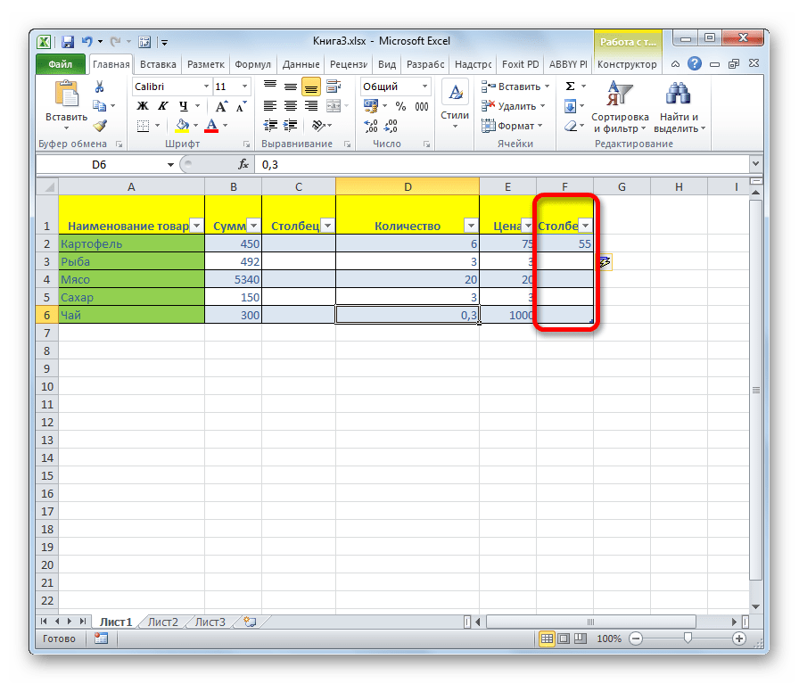
- Теперь для того, чтобы включить новый столбец в состав этой таблицы, достаточно заполнить любую ячейку справа от нее данными. Столбец, в котором находится данная ячейка, сразу станет табличным.


Как видим, существует целый ряд способов добавления новых столбцов на лист Excel как в середину таблицы, так и в крайние диапазоны. Чтобы добавление было максимально простым и удобным, лучше всего создать, так называемую «умную» таблицу. В этом случае, при добавлении данных в диапазон справа от таблицы он автоматически будет включен в неё в виде новой колонки.
Еще статьи по данной теме: