
This is a step-by-step guide on how to use IF function in Excel. It shows you how to create a formula using the IF function, it includes several IF formula examples, an introduction on how to use nested IF formulas, and the exercise file I used when creating this tutorial.
The Excel IF function performs a logical test and returns one value when the condition is TRUE and another when the condition is FALSE.
How do you write an if-then formula in Excel? Well, the syntax for IF statements is the same in all Excel versions. This means that you can use any of the examples shown in this article in Excel for Microsoft 365 or Excel 2021, 2019, 2016, 2013, 2010, 2007, and 2003.
How to use IF function in Excel:
- Select the cell where you want to insert the IF formula. Using your mouse or keyboard, navigate to the cell where you want to insert your formula.
- Type =IF(
- Insert the condition that you want to check, followed by a comma (,). The first argument of the IF function is the logical_test. This is the condition that you want to validate. For example C6 > 70.
- Insert the value to display when the condition is TRUE, followed by a comma (,). The second argument of the IF function is value_if_true. Here, you can insert a nested formula or a simple message such as “YES”.
- Insert the value to display when the condition is FALSE. The last argument of the IF function is value_if_false. Just like the previous step, you can insert a nested formula or display a message such as “NO”. This can also be set as an empty string (“”), which will display a cell that looks blank.
- Type ) to close the function and press ENTER
The following video shows you exactly how to apply the six steps described above and create your first IF formula.
The syntax that shows how to create an IF function in Excel is explained below:=IF(logical_test, [value_if_true], [value_if_false])
IF is a logical function and implies setting 3 arguments:
logical_test – The logical condition that you want to test. This will return either a TRUE or a FALSE value.
value_if_true – [optional] The value or formula which will be used when logical_test is TRUE.
value_if_false – [optional] The value or formula which will be used when logical_test is FALSE.
Please remember that while both value_if_true and value_if_false are optional, at least one of them needs to be supplied. Otherwise, your IF formula will simply return 0 (zero).
Where is the IF function in Excel? Since this is a logical function, you can find the IF function in the Formulas tab, Function Library section, under Logical.
Logical operators for IF function
The IF function is one of the most used Excel functions, and it allows you to return different values when the logical condition supplied is TRUE or FALSE. An Excel if-then formula can use the following logical operators:
| Logical operators | Definition | Example |
| = | equal to | A1=B1 |
| <> | not equal to | A1<>B1 |
| > | greater than | A1>B1 |
| >= | greater than or equal to | A1>=B1 |
| < | lower than | A1<B1 |
| <= | lower than or equal to | A1<=B1 |
The IF function doesn’t support wildcards.
Your first IF formula
The IF function runs a logical test and returns different values depending on whether the result is TRUE or FALSE. The result from IF can be a value, a cell reference, or even another formula.
Now let’s move on to some examples.
We’ll be evaluating exam grades. If the student obtained a score higher than or equal to 70, then we will return the message “Pass.” If the grade is lower than 70, then we will display “Fail.”
In this example, I have inserted the following formula in cell F9:=IF(E9>=70, "Pass", "Fail")
The 3 arguments for this IF formula are:
logical_test: E9>=70
value_if_true: Pass is returned if E9>=70.
value_if_false: Fail is returned if E9<70.

Please note that when you want to use text in your IF formulas (like a word or sentence), you need to wrap the text in quotes (e.g. “Fail”). The only exception is while using TRUE or FALSE, which are built-in functionalities that Excel recognizes automatically.
How to use the IF function in Excel with another function or formula
The beauty of the IF function is that it allows us to build complex financial models with lots of interdependencies. This includes using different formulas based on conditional logic.
In our next example, we will use the IF function to calculate a payment fee based on the value of the order. If the order value is higher than or equal to $1000, then it should calculate a payment fee of 1.00%. However, if the total order value is lower than $1000, then it should use 1.50%.
The formula in cell F31 is:=IF(E31>=1000, E31*1%, E31*1.5%)

Now let’s look at an IF formula that is dependent on user input. If we select free shipping for the order, then the shipping fee will be set to zero. Otherwise, it will be calculated as 3% of the order value.
This is something really easy to achieve, but it will open up so many opportunities for you to use the IF function in the future.

How to use nested IF statements in Excel
Nesting more IF functions allows you to perform multiple comparisons and create more complex formulas. However, you can only nest up to 64 IF functions in Excel. If you ever reach this limit (I never did), I can guarantee that there is a better and more elegant solution using functions like VLOOKUP, SUMIF, or COUNTIFS.
In the next example, I wrote a formula with several nested IF functions to assign a grade to a list of students based on their test results.
=IF(E71<60, "F", IF(E71<70, "D", IF(E71<80, "C", IF(E71<90, "B", "A"))))
The order of the conditions is important. When the conditions overlap, Excel will retrieve the [value_if_true] argument from the first IF statement that returns TRUE. This is why the conditions from the formula above need to be inserted in the same order for the formula to work properly.

Note: If you are running Office 365, then you can also look at the new IFS function. This function runs multiple tests and returns the value corresponding to the first TRUE result. It’s a very useful alternative to nested IF formulas and makes your formulas much easier to understand by others. You can read more about IFS on Microsoft’s website.
How to use IF formula with OR function in Excel
OR allows you to supply alternative conditions to an IF statement. This opens up opportunities to create complex scenarios where certain behavior is triggered by multiple possible conditions.
Let’s look at an IF formula that calculates a 2.00% shipping fee when the total order value is higher than $1000 or when there are more than 5 items in the order.
The IF OR statement I’ve used in cell H106 is:=IF(OR(G106>1000, F106>5), G106*2%, 0)

The OR function evaluates if G106>1000 or if F106>5 and the formula returns TRUE when either or both conditions are fulfilled.
How to use IF formula with AND function in Excel
AND allows you to supply multiple criteria to an IF statement. Basically, the IF function returns TRUE if, and only if, all the conditions are met.
Working with our previous example, let’s apply the shipping fee only when the total order value is higher than $1000 and the order contains more than 5 items.
The IF AND statement I’ve used in cell H106 is:=IF(AND(G128>1000, F128>5), G128*2%, 0)

The AND function evaluates if G106>1000 and if F106>5 and returns TRUE when both conditions are fulfilled.
How to use IF function with VLOOKUP in Excel
VLOOKUP can be nested inside an IF formula to retrieve data when a condition is TRUE or FALSE. In the next example, I will show you how to calculate shipping fees based on a different table that contains the thresholds and percentages to be applied depending on the order value.
The formula I’ve used in cell F152:=IF(G152="No", VLOOKUP(E152, $J$146:$K$152, 2, TRUE)*E152, 0)

The formula uses the following arguments:
logical_test: G152="No"
value_if_true: VLOOKUP(E152, $J$146:$K$152, 2, TRUE)*E152 is used to retrieve the corresponding shipping fee percentage when G152=”No”
value_if_false: 0 is returned if G152 is anything else than “No.” In our case, the alternative is selecting “Yes” from the drop-down list.
Note: One thing to remember is that I’ve used a VLOOKUP formula with an approximate match argument. This means that your data must be sorted in ascending order by lookup value (in our case, the Order amount).
In case you need additional help, please also read this article that explains step-by-step how to use VLOOKUP function in Excel.
What to do next?
IF is a versatile function that can be used in a wide range of scenarios. I use it daily, and I can’t imagine a world where Excel would lack this functionality.
Practice writing formulas using the IF function, and your spreadsheets will definitely get better and more complex. For example, why not look at another example using an IF function with 3 conditions? It will show you more examples of how to insert an if formula in Excel using nested IF statements and multiple conditions.
Let me know if you have questions on how to use IF function in Excel or if you need advice on how to nest multiple IF statements in your Excel project by leaving a comment below.
The logical IF statement in Excel is used for the recording of certain conditions. It compares the number and / or text, function, etc. of the formula when the values correspond to the set parameters, and then there is one record, when do not respond — another.
Logic functions — it is a very simple and effective tool that is often used in practice. Let us consider it in details by examples.
The syntax of the function «IF» with one condition
The operation syntax in Excel is the structure of the functions necessary for its operation data.
=IF(boolean;value_if_TRUE;value_if_FALSE)
Let us consider the function syntax:
- Boolean – what the operator checks (text or numeric data cell).
- Value_if_TRUE – what will appear in the cell when the text or numbers correspond to a predetermined condition (true).
- Value_if_FALSE – what appears in the box when the text or the number does not meet the predetermined condition (false).
Example:

Logical IF functions.
The operator checks the A1 cell and compares it to 20. This is a «Boolean». When the contents of the column is more than 20, there is a true legend «greater 20». In the other case it’s «less or equal 20».
Attention! The words in the formula need to be quoted. For Excel to understand that you want to display text values.
Here is one more example. To gain admission to the exam, a group of students must successfully pass a test. The results are listed in a table with columns: a list of students, a credit, an exam.

The statement IF should check not the digital data type but the text. Therefore, we prescribed in the formula В2= «done» We take the quotes for the program to recognize the text correctly.
The function IF in Excel with multiple conditions
Usually one condition for the logic function is not enough. If you need to consider several options for decision-making, spread operators’ IF into each other. Thus, we get several functions IF in Excel.
The syntax is as follows:
Here the operator checks the two parameters. If the first condition is true, the formula returns the first argument is the truth. False — the operator checks the second condition.
Examples of a few conditions of the function IF in Excel:

It’s a table for the analysis of the progress. The student received 5 points:
- А – excellent;
- В – above average or superior work;
- C – satisfactory;
- D – a passing grade;
- E – completely unsatisfactory.
IF statement checks two conditions: the equality of value in the cells.

In this example, we have added a third condition, which implies the presence of another report card and «twos». The principle of the operator is the same.
Enhanced functionality with the help of the operators «AND» and «OR»
When you need to check out a few of the true conditions you use the function И. The point is: IF A = 1 AND A = 2 THEN meaning в ELSE meaning с.
OR function checks the condition 1 or condition 2. As soon as at least one condition is true, the result is true. The point is: IF A = 1 OR A = 2 THEN value B ELSE value C.
Functions AND & OR can check up to 30 conditions.
An example of using the operator AND:

It’s the example of using the logical operator OR.

How to compare data in two tables
Users often need to compare the two spreadsheets in an Excel to match. Examples of the «life»: compare the prices of goods in different bringing, to compare balances (accounting reports) in a few months, the progress of pupils (students) of different classes, in different quarters, etc.
To compare the two tables in Excel, you can use the COUNTIFS statement. Consider the order of application functions.
For example, consider the two tables with the specifications of various food processors. We planned allocation of color differences. This problem in Excel solves the conditional formatting.
Baseline data (tables, which will work with):

Select the first table. Conditional Formatting — create a rule — use a formula to determine the formatted cells:

In the formula bar write: = COUNTIFS (comparable range; first cell of first table)=0. Comparing range is in the second table.
To drive the formula into the range, just select it first cell and the last. «= 0» means the search for the exact command (not approximate) values.
Choose the format and establish what changes in the cell formula in compliance. It’s better to do a color fill.
Select the second table. Conditional Formatting — create a rule — use the formula. Use the same operator (COUNTIFS). For the second table formula:
Download all examples in Excel

Now it is easy to compare the characteristics of the data in the table.
Функция ЕСЛИ в Excel — это отличный инструмент для проверки условий на ИСТИНУ или ЛОЖЬ. Если значения ваших расчетов равны заданным параметрам функции как ИСТИНА, то она возвращает одно значение, если ЛОЖЬ, то другое.
Содержание
- Что возвращает функция
- Синтаксис
- Аргументы функции
- Дополнительная информация
- Функция Если в Excel примеры с несколькими условиями
- Пример 1. Проверяем простое числовое условие с помощью функции IF (ЕСЛИ)
- Пример 2. Использование вложенной функции IF (ЕСЛИ) для проверки условия выражения
- Пример 3. Вычисляем сумму комиссии с продаж с помощью функции IF (ЕСЛИ) в Excel
- Пример 4. Используем логические операторы (AND/OR) (И/ИЛИ) в функции IF (ЕСЛИ) в Excel
- Пример 5. Преобразуем ошибки в значения “0” с помощью функции IF (ЕСЛИ)
Что возвращает функция
Заданное вами значение при выполнении двух условий ИСТИНА или ЛОЖЬ.
Синтаксис
=IF(logical_test, [value_if_true], [value_if_false]) — английская версия
=ЕСЛИ(лог_выражение; [значение_если_истина]; [значение_если_ложь]) — русская версия
Аргументы функции
- logical_test (лог_выражение) — это условие, которое вы хотите протестировать. Этот аргумент функции должен быть логичным и определяемым как ЛОЖЬ или ИСТИНА. Аргументом может быть как статичное значение, так и результат функции, вычисления;
- [value_if_true] ([значение_если_истина]) — (не обязательно) — это то значение, которое возвращает функция. Оно будет отображено в случае, если значение которое вы тестируете соответствует условию ИСТИНА;
- [value_if_false] ([значение_если_ложь]) — (не обязательно) — это то значение, которое возвращает функция. Оно будет отображено в случае, если условие, которое вы тестируете соответствует условию ЛОЖЬ.
Дополнительная информация
- В функции ЕСЛИ может быть протестировано 64 условий за один раз;
- Если какой-либо из аргументов функции является массивом — оценивается каждый элемент массива;
- Если вы не укажете условие аргумента FALSE (ЛОЖЬ) value_if_false (значение_если_ложь) в функции, т.е. после аргумента value_if_true (значение_если_истина) есть только запятая (точка с запятой), функция вернет значение “0”, если результат вычисления функции будет равен FALSE (ЛОЖЬ).
На примере ниже, формула =IF(A1> 20,”Разрешить”) или =ЕСЛИ(A1>20;»Разрешить») , где value_if_false (значение_если_ложь) не указано, однако аргумент value_if_true (значение_если_истина) по-прежнему следует через запятую. Функция вернет “0” всякий раз, когда проверяемое условие не будет соответствовать условиям TRUE (ИСТИНА).
 |
| - Если вы не укажете условие аргумента TRUE(ИСТИНА) (value_if_true (значение_если_истина)) в функции, т.е. условие указано только для аргумента value_if_false (значение_если_ложь), то формула вернет значение “0”, если результат вычисления функции будет равен TRUE (ИСТИНА);
На примере ниже формула равна =IF (A1>20;«Отказать») или =ЕСЛИ(A1>20;»Отказать»), где аргумент value_if_true (значение_если_истина) не указан, формула будет возвращать “0” всякий раз, когда условие соответствует TRUE (ИСТИНА).

Функция Если в Excel примеры с несколькими условиями
Пример 1. Проверяем простое числовое условие с помощью функции IF (ЕСЛИ)
При использовании функции ЕСЛИ в Excel, вы можете использовать различные операторы для проверки состояния. Вот список операторов, которые вы можете использовать:
Ниже приведен простой пример использования функции при расчете оценок студентов. Если сумма баллов больше или равна «35», то формула возвращает “Сдал”, иначе возвращается “Не сдал”.
Пример 2. Использование вложенной функции IF (ЕСЛИ) для проверки условия выражения
Функция может принимать до 64 условий одновременно. Несмотря на то, что создавать длинные вложенные функции нецелесообразно, то в редких случаях вы можете создать формулу, которая множество условий последовательно.
В приведенном ниже примере мы проверяем два условия.
- Первое условие проверяет, сумму баллов не меньше ли она чем 35 баллов. Если это ИСТИНА, то функция вернет “Не сдал”;
- В случае, если первое условие — ЛОЖЬ, и сумма баллов больше 35, то функция проверяет второе условие. В случае если сумма баллов больше или равна 75. Если это правда, то функция возвращает значение “Отлично”, в других случаях функция возвращает “Сдал”.
Пример 3. Вычисляем сумму комиссии с продаж с помощью функции IF (ЕСЛИ) в Excel
Функция позволяет выполнять вычисления с числами. Хороший пример использования — расчет комиссии продаж для торгового представителя.
В приведенном ниже примере, торговый представитель по продажам:
- не получает комиссионных, если объем продаж меньше 50 тыс;
- получает комиссию в размере 2%, если продажи между 50-100 тыс
- получает 4% комиссионных, если объем продаж превышает 100 тыс.
Рассчитать размер комиссионных для торгового агента можно по следующей формуле:
=IF(B2<50,0,IF(B2<100,B2*2%,B2*4%)) — английская версия
=ЕСЛИ(B2<50;0;ЕСЛИ(B2<100;B2*2%;B2*4%)) — русская версия
В формуле, использованной в примере выше, вычисление суммы комиссионных выполняется в самой функции ЕСЛИ. Если объем продаж находится между 50-100K, то формула возвращает B2 * 2%, что составляет 2% комиссии в зависимости от объема продажи.
Больше лайфхаков в нашем Telegram Подписаться
Пример 4. Используем логические операторы (AND/OR) (И/ИЛИ) в функции IF (ЕСЛИ) в Excel
Вы можете использовать логические операторы (AND/OR) (И/ИЛИ) внутри функции для одновременного тестирования нескольких условий.
Например, предположим, что вы должны выбрать студентов для стипендий, основываясь на оценках и посещаемости. В приведенном ниже примере учащийся имеет право на участие только в том случае, если он набрал более 80 баллов и имеет посещаемость более 80%.
Вы можете использовать функцию AND (И) вместе с функцией IF (ЕСЛИ), чтобы сначала проверить, выполняются ли оба эти условия или нет. Если условия соблюдены, функция возвращает “Имеет право”, в противном случае она возвращает “Не имеет право”.
Формула для этого расчета:
=IF(AND(B2>80,C2>80%),”Да”,”Нет”) — английская версия
=ЕСЛИ(И(B2>80;C2>80%);»Да»;»Нет») — русская версия
Пример 5. Преобразуем ошибки в значения “0” с помощью функции IF (ЕСЛИ)
С помощью этой функции вы также можете убирать ячейки содержащие ошибки. Вы можете преобразовать значения ошибок в пробелы или нули или любое другое значение.
Формула для преобразования ошибок в ячейках следующая:
=IF(ISERROR(A1),0,A1) — английская версия
=ЕСЛИ(ЕОШИБКА(A1);0;A1) — русская версия
Формула возвращает “0”, в случае если в ячейке есть ошибка, иначе она возвращает значение ячейки.
ПРИМЕЧАНИЕ. Если вы используете Excel 2007 или версии после него, вы также можете использовать функцию IFERROR для этого.
Точно так же вы можете обрабатывать пустые ячейки. В случае пустых ячеек используйте функцию ISBLANK, на примере ниже:
=IF(ISBLANK(A1),0,A1) — английская версия
=ЕСЛИ(ЕПУСТО(A1);0;A1) — русская версия
What is IF Function in Excel?
IF function in Excel evaluates whether a given condition is met and returns a value depending on whether the result is “true” or “false”. It is a conditional function of Excel, which returns the result based on the fulfillment or non-fulfillment of the given criteria.
For example, the IF formula in Excel can be applied as follows:
“=IF(condition A,“value B”,“value C”)”
The IF excel function returns “value B” if condition A is met and returns “value C” if condition A is not met.
It is often used to make logical interpretations which help in decision-making.
Table of contents
- What is IF Function in Excel?
- Syntax of the IF Excel Function
- How to Use IF Function in Excel?
- Example #1
- Example #2
- Example #3
- Example #4
- Example #5
- Guidelines for the Multiple IF Statements
- Frequently Asked Question
- IF Excel Function Video
- Recommended Articles
Syntax of the IF Excel Function
The syntax of the IF function is shown in the following image:

The IF excel function accepts the following arguments:
- Logical_test: It refers to the condition to be evaluated. The condition can be a value or a logical expression.
- Value_if_true: It is the value returned as a result when the condition is “true”.
- Value_if_false: It is the value returned as a result when the condition is “false”.
In the formula, the “logical_test” is a required argument, whereas the “value_if_true” and “value_if_false” are optional arguments.
The IF formula uses logical operators to evaluate the values in a range of cells. The following table shows the different logical operatorsLogical operators in excel are also known as the comparison operators and they are used to compare two or more values, the return output given by these operators are either true or false, we get true value when the conditions match the criteria and false as a result when the conditions do not match the criteria.read more and their meaning.
| Operator | Meaning |
|---|---|
| = | Equal to |
| > | Greater than |
| >= | Greater than or equal to |
| < | Less than |
| <= | Less than or equal to |
| <> | Not equal to |
How to Use IF Function in Excel?
Let us understand the working of the IF function with the help of the following examples in Excel.
You can download this IF Function Excel Template here – IF Function Excel Template
Example #1
If there is no oxygen on a planet, life is impossible. If oxygen is available on a planet, then life is possible. The following table shows a list of planets in column A and the information on the availability of oxygen in column B. We have to find the planets where life is possible, based on the condition of oxygen availability.

Let us apply the IF formula to cell C2 to find out whether life is possible on the planets listed in the table.
The IF formula is stated as follows:
“=IF(B2=“Yes”, “Life is Possible”, “Life is Not Possible”)
The succeeding image shows the IF formula applied to cell C2.

The subsequent image shows how the IF formula is applied to the range of cells C2:C5.

Drag the cells to view the output of all the planets.

The output in the below worksheet shows life is possible on the planet Earth.
Flow Chart of Generic IF Excel Function

The IF Function Flow Chart for Mars (Example #1)

The flow of IF function flowchart for Jupiter and Venus is the same as the IF function flowchart for Mars (Example #1).
The IF Function Flow Chart for Earth

Hence, the IF excel function allows making logical comparisons between values. The modus operandi of the IF function is stated as: If something is true, then do something; otherwise, do something else.
Example #2
The following table shows a list of years. We want to find out if the given year is a leap year or not.
A leap year has 366 days; the extra day is the 29th of February. The criteria for a leap year are stated as follows:
- The year will be exactly divisible by 4 and not exactly be divisible by 100 or
- The year will be exactly divisible by 400.

In this example, we will use the IF function along with the AND, OR, and MOD functions to find the leap years.
We use the MOD function to find a remainder after a dividend is divided by a divisor.
The AND functionThe AND function in Excel is classified as a logical function; it returns TRUE if the specified conditions are met, otherwise it returns FALSE.read more evaluates both the conditions of the leap years for the value “true”. The OR functionThe OR function in Excel is used to test various conditions, allowing you to compare two values or statements in Excel. If at least one of the arguments or conditions evaluates to TRUE, it will return TRUE. Similarly, if all of the arguments or conditions are FALSE, it will return FASLE.read more evaluates either of the condition for the value “true”.
We will apply the MOD function to the conditions as follows:
If MOD(year,4)=0 and MOD(year,100)<>(is not equal to) 0, then the year is a leap year.
or
If MOD(year,400)=0, then the year is a leap year; otherwise, the year is not a leap year.
The IF formula is stated as follows:
“=IF(OR(AND((MOD(year,4)=0),(MOD(year,100)<>0)),(MOD(year,400)=0)),“Leap Year”, “Not A Leap Year”)”
The argument “year” refers to a reference value.
The following images show the output of the IF formula applied in the range of cells.


The following image shows how the IF formula is applied to the range of cells B2:B18.

The succeeding table shows the years 1960, 2028, and 2148 as leap years and the remaining as non-leap years.

The result of the IF excel formula is displayed for the range of cells B2:B18 in the following image.

Example #3
The succeeding table shows a list of drivers and the directions they undertook to reach the destination. It is preceded by an image of the road intersection explaining the turns taken by the drivers and their destinations. The right turn leads to town B, and the left turn leads to town C. Identify the driver’s destination to town B and town C.
Road Intersection Image


Let us apply the IF excel function to find the destination. Here, the condition is mentioned as follows:
- If the driver turns right, he/she reaches town B.
- If the driver turns left, he/she reaches town C.
We use the following IF formula to find the destination:
“=IF(B2=“Left”, “Town C”, “Town B”)”
The succeeding image shows the output of the IF formula applied to cell C2.

Drag the cells to use the formula in the range C2:C11. Finally, we get the destinations of each driver for their turning movements.
The below image displays the IF formula applied to the range.

The output of the IF formula and the destinations are displayed in the succeeding image.

The result shows that six drivers reached town C, and the remaining four have reached town B.
Example #4
The following table shows a list of items and their inventory levels. We want to check if the specific item is available in the inventory or not using the IF function.

Let us list the name of items in column A and the number of items in column B. The list of data to be validated for the entire items list is shown in the cell E2 of the below image.

We use the Excel IF along with the VLOOKUP functionThe VLOOKUP excel function searches for a particular value and returns a corresponding match based on a unique identifier. A unique identifier is uniquely associated with all the records of the database. For instance, employee ID, student roll number, customer contact number, seller email address, etc., are unique identifiers.
read more to check the availability of the items in the inventory.
The VLOOKUP function looks up the values referring to the number of items, and the IF function will check whether the item number is greater than zero or not.
We will apply the following IF formula in the F2 cell:
“=IF(VLOOKUP(E2,A2:B11,2,0)=0, “Item Not Available”,“Item Available”)”
If the lookup value of an item is equal to 0, then the item is not available; else, the item is available.
The succeeding image shows the result of the IF formula in the cell F2.

Select “bat” in the E2 item cell to know whether the item is available or not in the inventory (as shown in the following image).

Example #5
The following table shows the list of students and their marks. The grade criteria are provided based on the marks obtained by the students. We want to find the grade of each student in the list.

We apply the Nested IF in Excel since we have multiple criteria to find and decide each student’s grade.
The Nesting of IF function uses the IF function inside another IF formula when multiple conditions are to be fulfilled.
The syntax of Nesting of IF function is stated as follows:
“=IF( condition1, value_if_true1, IF( condition2, value_if_true2, value_if_false2 ))”
The succeeding table represents the range of scores and the grades, respectively.

Let us apply the multiple IF conditions with AND function in the below-nested formula to find out the grade of the students:
“=IF((B2>=95),“A”,IF(AND(B2>=85,B2<=94),“B”,IF(AND(B2>=75,B2<=84),“C”,IF(AND(B2>=61,B2<=74),“D”,“F”))))”
The IF function checks the logical condition as shown in the formula below:
“=IF(logical_test, [value_if_true],[value_if_false])”
We will split the above-mentioned nested formula and check the IF statements as shown below:
First Logical Test: B2>=95
If the formula returns,
- Value_if_true, execute: “A” (Grade A) else(comma) enter value_if_false
- Value_if_false, then the formula finds another IF condition and enter IF condition
Second Logical Test: B2>=85(logical expression 1) and B2<=94(logical expression 2)
(We use AND function to check the multiple logical expressions as the two given conditions are to be evaluated for “true.”)
If the formula returns,
- Value_if_true, execute: “B” (Grade B) else(comma) enter value_if_false
- Value_if_false, then the formula finds another IF condition and enter IF condition
Third Logical Test: B2>=75(logical expression 1) and B2<=84(logical expression 2)
(We use AND function to check the multiple logical expressions as the two given conditions are to be evaluated for “true.”)
If the formula returns,
- Value_if_true, execute: “C” (Grade C) else(comma) enter value_if_false
- value_if_false, then the formula finds another IF condition and enter IF condition
Fourth Logical Test: B2>=61(logical expression 1) and B2<=74(logical expression 2)
(We use AND function to check the multiple logical expressions as the two given conditions are to be evaluated for “true.”)
If the formula returns,
- Value_if_true, execute: “D” (Grade D) else(comma) enter value_if_false
- Value_if_false, execute: “F” (Grade F)
- Finally, close the parenthesis.
The below image displays the output of the IF formula applied to the range.

The succeeding image shows the IF nested formula applied to the range.

The grades of the students are listed in the following table.

Guidelines for the Multiple IF Statements
The guidelines for the multiple IF statements are listed as follows:
- Use nested IF function to a limited extent as multiple IF statements require a great deal of thought to be accurate.
- Multiple IF statementsIn Excel, multiple IF conditions are IF statements that are contained within another IF statement. They are used to test multiple conditions at the same time and return distinct values. Additional IF statements can be included in the ‘value if true’ and ‘value if false’ arguments of a standard IF formula.read more require multiple parentheses (), which is often difficult to manage. Excel provides a way to check the color of each opening and closing parenthesis to avoid this situation. The last closing parenthesis color will always be black, denoting the end of the formula statement.
- Whenever we pass a string value for the arguments “value_if_true” and “value_if_false” or test a reference against a string value, enclose the string value in double quotes. Passing a string value without quotes will result in “#NAME?” error.
Frequently Asked Question
1. What is the IF function in Excel?
The Excel IF function is a logical function that checks the given criteria and returns one value for a “true” and another value for a “false” result.
The syntax of the IF function is stated as follows:
“=IF(logical_test, [value_if_true], [value_if_false])”
The arguments are as follows:
1. Logical_test – It refers to a value or condition that is tested.
2. Value_if_true – It is the value returned when the condition logical_test is “true.”
3. Value_if_false – It is the value returned when the condition logical_test is “false.”
The “logical_test” is a required argument, whereas the “value_if_true” and “value_if_false” are optional arguments.
2. How to use the IF Excel function with multiple conditions?
The IF Excel statement for multiple conditions is created by using multiple IF functions in a single formula.
The syntax of IF function with multiple conditions is stated as follows:
“=IF (condition 1_“true”, do something, IF (condition 2_“true”, do something, IF (condition 3_ “true”, do something, else do something)))”
3. How to use the function IFERROR in Excel?
IF Excel Function Video
Recommended Articles
This has been a guide to the IF function in Excel. Here we discuss how to use the IF function along with examples and downloadable templates. You may also look at these useful functions –
- What is the Logical Test in Excel?A logical test in Excel results in an analytical output, either true or false. The equals to operator, “=,” is the most commonly used logical test.read more
- “Not Equal to” in Excel“Not Equal to” argument in excel is inserted with the expression <>. The two brackets posing away from each other command excel of the “Not Equal to” argument, and the user then makes excel checks if two values are not equal to each other.read more
- Data Validation ExcelThe data validation in excel helps control the kind of input entered by a user in the worksheet.read more
The IF function is useful for making quick decisions or performing comparisons in Microsoft Excel. It’s an easy but versatile logical comparison function for handling many scenarios, ranging from financial models to assigning allowances. In this tutorial, I’ll show how to use the IF function in Excel and a simple adaptation. (Includes practice worksheet)
What is the IF Function?
The IF function is one of the simplest and most useful logical functions. It can fill cell items for you based on evaluating a condition such as a cell’s content and logical operators. What’s appealing about the function is that it can be used with other functions to handle more complex scenarios. You might think of it as a formula building block and you can find it in the Logical category.
The wizard-like dialog allows you to fill 3 Function Arguments or data elements, but you could use the formula bar once you master it. This is the easiest way to learn an Excel formula because you can see if it returns your expected result. For example, at the bottom left of the dialog, a line reads “Formula result =.”
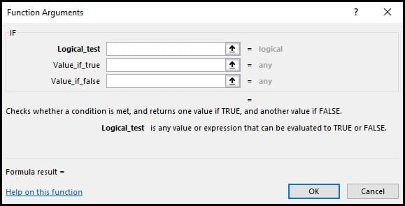
The IF Function Arguments
| Field | Definition |
|---|---|
| Logical_test | A test on a cell value that is either TRUE or FALSE. |
| Value_if_true | The value Excel will put in a cell if the test is true. |
| Value_if_false | The value Excel will put in a cell if the test fails. |
Despite not having Microsoft Excel, my parents routinely employed this type of IF logic when calculating my allowance. Their version read:
IF you empty the garbage AND mow the lawn AND wash the dishes AND walk the dog, you get your full allowance.
And since I grew up in New England, this logic would change with the seasons to account for leaves and snow.
Setting Up the IF Function
Although Excel can’t issue an allowance, it can calculate the amount using a logic test based on whether a cell met a formula condition.
For example, I could create a spreadsheet with the chores needed to get an allowance. If the chores were completed (TRUE situation), a value would be applied toward the allowance. If the chore wasn’t completed (FALSE situation), nothing would be added.
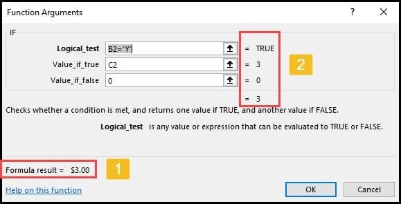
These examples are noted by labels [1] and [2] in the screen snap below.

Using the example above, you might express the logic in the following way:
IF cell B2 equals “Y”, then use the Rate value from cell C2 ($3.00) in D2.
IF cell B2 does not equal “Y”, then place 0 in cell D2.
As you can see in this example, the IF logical condition is either TRUE or FALSE. And it pays to take out the garbage.
Comparison Operators
To help evaluate conditions, Excel uses a list of common operators. You probably know these as we probably used them in math class. These operators will be evaluated to a logical “true” or “false”. In the table below, B2 and C2 in the Example column are cell references.
| Operator | Example |
| = (equals) | B2 = “YES” |
| < (less than) | B2 < 12 |
| > (greater than) | B2 > 112 |
| <= (less than or equal to) | B2 <= 12 |
| >= (greater than or equal to) | B2 >= 12 |
| <> (not equal to) | B2 <> C2 |
How To Enter IF Function Arguments
- Click the spreadsheet cell where you wish to use the Excel formula.
- From the Formulas tab, click Insert function…
- In the Insert Function dialog text box, type “if“.
Note: On Office 365, there is now a Logical button on the Formulas tab. You can select IF from the drop-down menu.
- Make sure your cursor is in the Logical_test text box.
- Click the spreadsheet cell you wish to evaluate. Excel will fill in the cell reference such as “B2”.
- Add the equals sign = and your desired value in quotes. For example =”Y”.
- In the Value_if_true field, type the value you would like entered in your cell if B2 equals “Y”. In our example, I’ll click cell C3.
- In the Value_if_false: field, enter the value the cell should have if B2 does not have a “Y”. I’ll enter 0. I could leave it blank, but the cell would show “FALSE”.
- Review the dialog to see if the Formula result= value (label [1] below) is what you expect. If not, check to see if any errors show to the right of the fields (label [2] below).
- Click OK.
- Copy the formula to the other cells in your column.
✪ Tip: Even though the Value_if_false field is optional, it’s best to provide a value. Otherwise, Excel will use FALSE in the cell value.
Excel IF With Numeric Values
The above spreadsheet might have been Version 1 for my parents. A new incentive program would appear based on some parent/child negotiations and competitive neighborhood rates. I probably would’ve requested pay for partial chores. No doubt, my parents would counter with a penalty clause if something was less than half done.
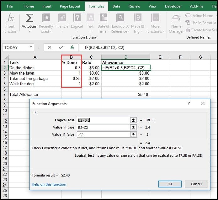
Excel is flexible when it comes to IF statements and can evaluate more than a simple “Y” or “N.” For example, if we convert our previous Done? column to a % Done column with a number, we can accommodate these new requirements such as:
=IF(B2>0.5,B2*C2,-C2)The new formula returns the allowance based on the % Done in Column B. If the chore completion number is greater than .5, a prorated amount is applied to the allowance.
If the chore completion rate was .5 or below, a negative amount was applied to the allowance. Loosely translated, an “incomplete” performance costs money. You could also apply colors using conditional formatting.
Troubleshooting Tips
There are a couple of reasons why the IF function doesn’t work as expected.
- You don’t have quotes around a text string. For example, you used B2=Y instead of B2=”Y”. The quotes aren’t needed if you use the values TRUE or FALSE as Excel recognizes them.
- You have a data type mismatch. For example, your comparison operator was comparing a number in one cell such as “twelve”, but the comparison cell had 12. However, Excel is forgiving if you’re evaluating number formats such as 1.5 versus $1.50.
As you’ve seen, this is a versatile and useful function. Once you get the hang of how to use IF function in Excel, you’ll start using it in more scenarios. The two examples presented here were foundational. But you can use IF functions to handle other transactions such as applying sales tax, stock values, shipping charges, fixing Excel DIV 0 errors, or even nesting IF functions with Boolean logic.
And if you have kids, let them build the Excel spreadsheet and give them a bonus for using the IF function.
Hand-picked Excel Tutorials
- How to Use Excel VLOOKUP
- Beginner’s Guide to XLOOKUP
- How to Create an Excel Pivot Table
- The Benefits of Creating Excel Tables
- Video: How to Use Conditional Formatting