Inputting data on excel - Word и Excel - помощь в работе с программами

Содержание

Apply data validation to cells
Try it!
Download our examples
Restrict data entry
Prompt users for valid entries
Display an error message when invalid data is entered
Add data validation to a cell or a range
How to Create a Data Entry Form in Excel (Step-by-step Guide)
Why Do You Need to Know About Data Entry Forms?
Data Entry Form in Excel
Adding Data Entry Form Option To Quick Access Toolbar
Parts of the Data Entry Form
Creating a New Entry
Navigating Through Existing Records
Deleting a Record
Restricting Data Entry Based on Rules

Apply data validation to cells

Use data validation to restrict the type of data or the values that users enter into a cell. One of the most common data validation uses is to create a drop-down list.

Try it!

Select the cell(s) you want to create a rule for.

Select Data >Data Validation.

On the Settings tab, under Allow, select an option:

Whole Number — to restrict the cell to accept only whole numbers.

Decimal — to restrict the cell to accept only decimal numbers.

List — to pick data from the drop-down list.

Date — to restrict the cell to accept only date.

Time — to restrict the cell to accept only time.

Text Length — to restrict the length of the text.

Custom – for custom formula.

Under Data, select a condition.

Set the other required values based on what you chose for Allow and Data.

Select the Input Message tab and customize a message users will see when entering data.

Select the Show input message when cell is selected checkbox to display the message when the user selects or hovers over the selected cell(s).

Select the Error Alert tab to customize the error message and to choose a Style.

Now, if the user tries to enter a value that is not valid, an Error Alert appears with your customized message.

Download our examples

If you’re creating a sheet that requires users to enter data, you might want to restrict entry to a certain range of dates or numbers, or make sure that only positive whole numbers are entered. Excel can restrict data entry to certain cells by using data validation, prompt users to enter valid data when a cell is selected, and display an error message when a user enters invalid data.

Restrict data entry

Select the cells where you want to restrict data entry.

On the Data tab, click Data Validation > Data Validation.

Note: If the validation command is unavailable, the sheet might be protected or the workbook might be shared. You cannot change data validation settings if your workbook is shared or your sheet is protected. For more information about workbook protection, see Protect a workbook.

In the Allow box, select the type of data you want to allow, and fill in the limiting criteria and values.

Note: The boxes where you enter limiting values will be labeled based on the data and limiting criteria that you have chosen. For example, if you choose Date as your data type, you will be able to enter limiting values in minimum and maximum value boxes labeled Start Date and End Date.

Prompt users for valid entries

When users click in a cell that has data entry requirements, you can display a message that explains what data is valid.

Select the cells where you want to prompt users for valid data entries.

On the Data tab, click Data Validation > Data Validation.

On the Input Message tab, select the Show input message when cell is selected check box.

In the Title box, type a title for your message.

In the Input message box, type the message that you want to display.

Display an error message when invalid data is entered

If you have data restrictions in place and a user enters invalid data into a cell, you can display a message that explains the error.

Select the cells where you want to display your error message.

On the Data tab, click Data Validation > Data Validation.

On the Error Alert tab, in the Title box, type a title for your message.

In the Error message box, type the message that you want to display if invalid data is entered.

Do one of the following:

On the Style pop-up menu, select

Require users to fix the error before proceeding

Warn users that data is invalid, and require them to select Yes or No to indicate if they want to continue

Warn users that data is invalid, but allow them to proceed after dismissing the warning message

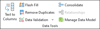
Add data validation to a cell or a range

Note: The first two steps in this section are for adding any type of data validation. Steps 3-7 are specifically for creating a drop-down list.

Select one or more cells to validate.

On the Data tab, in the Data Tools group, click Data Validation.

On the Settings tab, in the Allow box, select List.

In the Source box, type your list values, separated by commas. For example, type Low,Average,High.

Make sure that the In-cell dropdown check box is selected. Otherwise, you won’t be able to see the drop-down arrow next to the cell.

To specify how you want to handle blank (null) values, select or clear the Ignore blank check box.

Test the data validation to make sure that it is working correctly. Try entering both valid and invalid data in the cells to make sure that your settings are working as you intended and your messages are appearing when you expect.

After you create your drop-down list, make sure it works the way you want. For example, you might want to check to see if the cell is wide enough to show all your entries.

Remove data validation — Select the cell or cells that contain the validation you want to delete, then go to Data > Data Validation and in the data validation dialog press the Clear All button, then click OK.

The following table lists other types of data validation and shows you ways to add it to your worksheets.

Follow these steps:

Restrict data entry to whole numbers within limits.

Follow steps 1-2 above.

From the Allow list, select Whole number.

In the Data box, select the type of restriction that you want. For example, to set upper and lower limits, select between.

Enter the minimum, maximum, or specific value to allow.

You can also enter a formula that returns a number value.

For example, say you’re validating data in cell F1. To set a minimum limit of deductions to two times the number of children in that cell, select greater than or equal to in the Data box and enter the formula, =2*F1, in the Minimum box.

Restrict data entry to a decimal number within limits.

Follow steps 1-2 above.

In the Allow box, select Decimal.

In the Data box, select the type of restriction that you want. For example, to set upper and lower limits, select between.

Enter the minimum, maximum, or specific value to allow.

You can also enter a formula that returns a number value. For example, to set a maximum limit for commissions and bonuses of 6% of a salesperson’s salary in cell E1, select less than or equal to in the Data box and enter the formula, =E1*6%, in the Maximum box.

Note: To let a user enter percentages, for example 20%, select Decimal in the Allow box, select the type of restriction that you want in the Data box, enter the minimum, maximum, or specific value as a decimal, for example .2, and then display the data validation cell as a percentage by selecting the cell and clicking Percent Style in the Number group on the Home tab.

Restrict data entry to a date within range of dates.

Follow steps 1-2 above.

In the Allow box, select Date.

In the Data box, select the type of restriction that you want. For example, to allow dates after a certain day, select greater than.

Enter the start, end, or specific date to allow.

You can also enter a formula that returns a date. For example, to set a time frame between today’s date and 3 days from today’s date, select between in the Data box, enter =TODAY() in the Start date box, and enter =TODAY()+3 in the End date box.

Restrict data entry to a time within a time frame.

Follow steps 1-2 above.

In the Allow box, select Time.

In the Data box, select the type of restriction that you want. For example, to allow times before a certain time of day, select less than.

Enter the start, end, or specific time to allow. If you want to enter specific times, use the hh:mm time format.

For example, say you have cell E2 set up with a start time (8:00 AM), and cell F2 with an end time (5:00 PM), and you want to limit meeting times between those times then select between in the Data box, enter =E2 in the Start time box, and then enter =F2 in the End time box.

Restrict data entry to text of a specified length.

Follow steps 1-2 above.

In the Allow box, select Text Length.

In the Data box, select the type of restriction that you want. For example, to allow up to a certain number of characters, select less than or equal to.

In this case we want to limit entry to 25 characters, so select less than or equal to in the Data box and enter 25 in the Maximum box.

Calculate what is allowed based on the content of another cell.

Follow steps 1-2 above.

In the Allow box, select the type of data that you want.

In the Data box, select the type of restriction that you want.

In the box or boxes below the Data box, click the cell that you want to use to specify what is allowed.

For example, to allow entries for an account only if the result won’t go over the budget in cell E1, select Allow > Whole number, Data, less than or equal to, and Maximum >= =E1.

The following examples use the Custom option where you write formulas to set your conditions. You don’t need to worry about whatever the Data box shows, as that’s disabled with the Custom option.

The screen shots in this article were taken in Excel 2016; but the functionality is the same in Excel for the web.

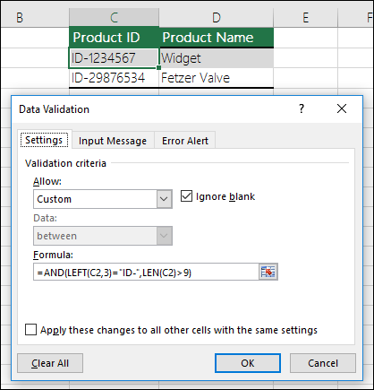
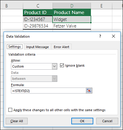
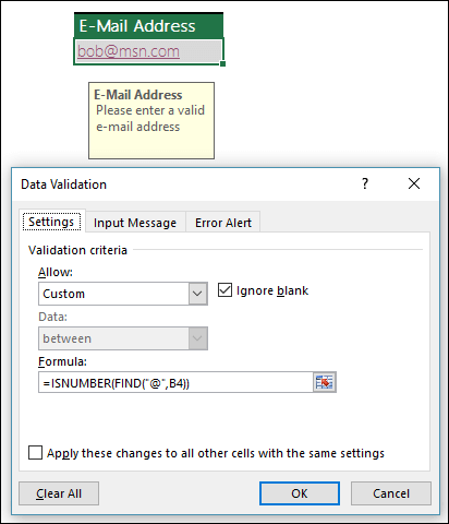
To make sure that

Enter this formula

The cell that contains a product ID (C2) always begins with the standard prefix of «ID-» and is at least 10 (greater than 9) characters long.

The cell that contains a product name (D2) only contains text.

The cell that contains someone’s birthday (B6) has to be greater than the number of years set in cell B4.

Note: You must enter the data validation formula for cell A2 first, then copy A2 to A3:A10 so that the second argument to the COUNTIF will match the current cell. That is the A2)=1 portion will change to A3)=1, A4)=1 and so on.

For more information

Ensure that an e-mail address entry in cell B4 contains the @ symbol.

Tip: If you’re a small business owner looking for more information on how to get Microsoft 365 set up, visit Small business help & learning.

Источник

How to Create a Data Entry Form in Excel (Step-by-step Guide)

Watch the Video on Using Data Entry Forms in Excel

Below is a detailed written tutorial about Excel Data Entry form in case you prefer reading over watching a video.

Excel has many useful features when it comes to data entry.

And one such feature is the Data Entry Form.

In this tutorial, I will show you what are data entry forms and how to create and use them in Excel.

This Tutorial Covers:

Why Do You Need to Know About Data Entry Forms?

But if data entry is a part of your daily work, I recommend you check out this feature and see how it can help you save time (and make you more efficient).

There are two common issues that I have faced (and seen people face) when it comes to data entry in Excel:

It’s time-consuming. You need to enter the data in one cell, then go to the next cell and enter the data for it. Sometimes, you need to scroll up and see which column it is and what data needs to be entered. Or scroll to the right and then come back to the beginning in case there are many columns.
It’s error-prone. If you have a huge data set which needs 40 entries, there is a possibility you may end up entering something that was not intended for that cell.

A data entry form can help by making the process faster and less error-prone.

Before I show you how to create a data entry form in Excel, let me quickly show you what it does.

Below is a data set that is typically maintained by the hiring team in an organization.

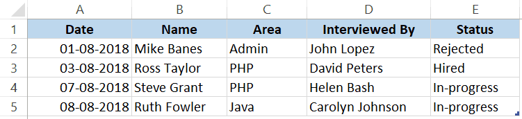
Every time a user has to add a new record, he/she will have to select the cell in the next empty row and then go cell by cell to make the entry for each column.

While this is a perfectly fine way of doing it, a more efficient way would be to use a Data Entry Form in Excel.

Below is a data entry form that you can use to make entries to this data set.

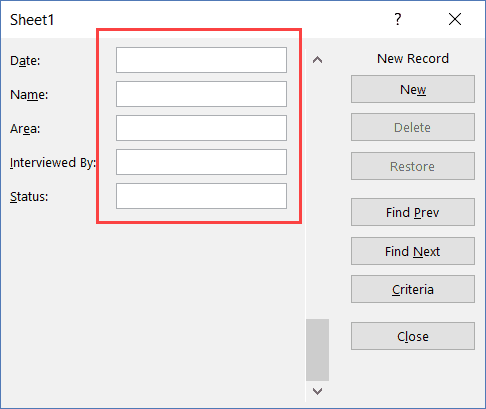
The highlighted fields are where you would enter the data. Once done, hit the Enter key to make the data a part of the table and move on to the next entry.

Below is a demo of how it works:

As you can see, this is easier than regular data entry as it has everything in a single dialog box.

Data Entry Form in Excel

Using a data entry form in Excel needs a little pre-work.

You would notice that there is no option to use a data entry form in Excel (not in any tab in the ribbon).

To use it, you will have to first add it to the Quick Access Toolbar (or the ribbon).

Adding Data Entry Form Option To Quick Access Toolbar

Below are the steps to add the data entry form option to the Quick Access Toolbar:

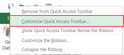
Right-click on any of the existing icons in the Quick Access Toolbar.
Click on ‘Customize Quick Access Toolbar’.
In the ‘Excel Options’ dialog box that opens, select the ‘All Commands’ option from the drop-down.
Scroll down the list of commands and select ‘Form’.
Click on the ‘Add’ button.
Click OK.

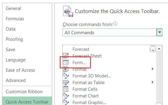
The above steps would add the Form icon to the Quick Access Toolbar (as shown below).

Once you have it in QAT, you can click any cell in your dataset (in which you want to make the entry) and click on the Form icon.

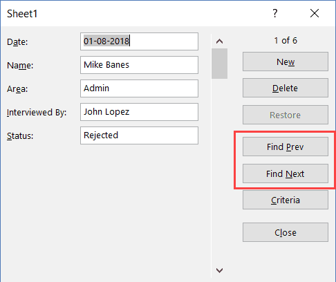
Parts of the Data Entry Form

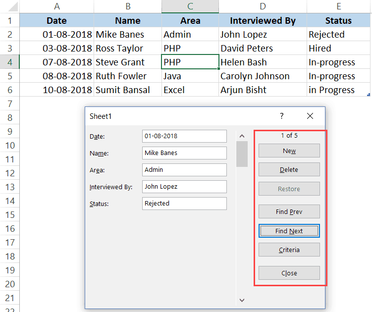
A Data Entry Form in Excel has many different buttons (as you can see below).

Here is a brief description of what each button is about:

New: This will clear any existing data in the form and allows you to create a new record.
Delete: This will allow you to delete an existing record. For example, if I hit the Delete key in the above example, it will delete the record for Mike Banes.
Restore: If you’re editing an existing entry, you can restore the previous data in the form (if you haven’t clicked New or hit Enter).
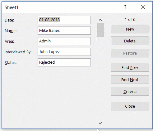
Find Prev: This will find the previous entry.
Find Next: This will find the next entry.
Criteria: This allows you to find specific records. For example, if I am looking for all the records, where the candidate was Hired, I need to click the Criteria button, enter ‘Hired’ in the Status field and then use the find buttons. Example of this is covered later in this tutorial.
Close: This will close the form.
Scroll Bar: You can use the scroll bar to go through the records.

Now let’s go through all the things you can do with a Data Entry form in Excel.

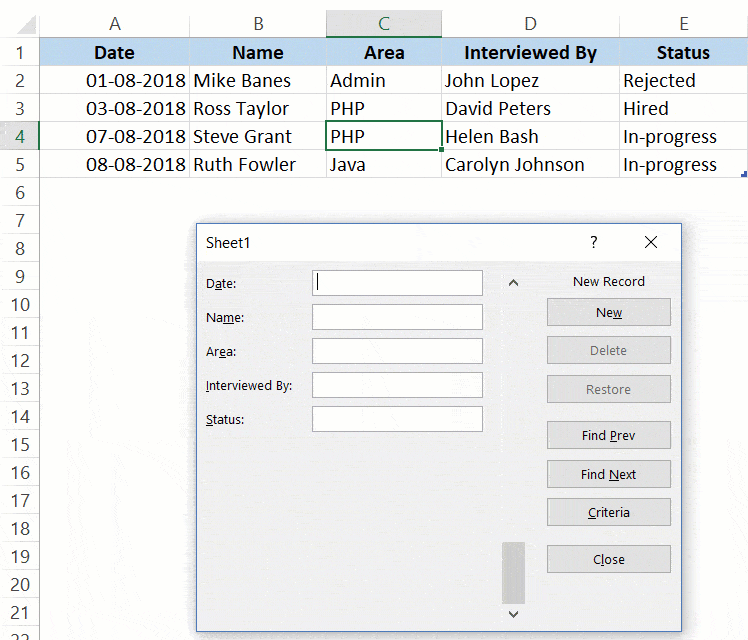
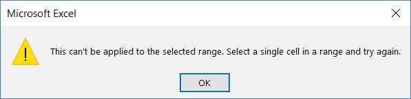
Note that you need to convert your data into an Excel Table and select any cell in the table to be able to open the Data Entry form dialog box.

If you haven’t selected a cell in the Excel Table, it will show a prompt as shown below:

Creating a New Entry

Below are the steps to create a new entry using the Data Entry Form in Excel:

Select any cell in the Excel Table.
Click on the Form icon in the Quick Access Toolbar.
Enter the data in the form fields.
Hit the Enter key (or click the New button) to enter the record in the table and get a blank form for next record.

Navigating Through Existing Records

One of the benefits of using Data Entry Form is that you can easily navigate and edit the records without ever leaving the dialog box.

This can be especially useful if you have a dataset with many columns. This can save you a lot of scrolling and the process of going back and forth.

Below are the steps to navigate and edit the records using a data entry form:

Select any cell in the Excel Table.
Click on the Form icon in the Quick Access Toolbar.
To go to the next entry, click on the ‘Find Next’ button and to go to the previous entry, click the ‘Find Prev’ button.
To edit an entry, simply make the change and hit enter. In case you want to revert to the original entry (if you haven’t hit the enter key), click the ‘Restore’ button.

You can also use the scroll bar to navigate through entries one-by-one.

The above snapshot shows basic navigation where you are going through all the records one after the other.

But you can also quickly navigate through all the records based on criteria.

For example, if you want to go through all the entries where the status is ‘In-progress’, you can do that using the below steps:

Select any cell in the Excel table.
Click on the Form icon in the Quick Access Toolbar.
In the Data Entry Form dialog box, click the Criteria button.
In the Status field, enter ‘In-progress’. Note that this value is not case sensitive. So even if you enter IN-PROGRESS, it would still work.
Use the Find Prev/Find Next buttons to navigate through the entries where the status is In-Progress.

Criteria is a very useful feature when you have a huge dataset, and you want to quickly go through those records that meet a given set of criteria.

Note that you can use multiple criteria fields to navigate through the data.

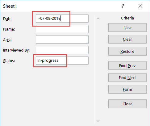
For example, if you want to go through all the ‘In-progress’ records after 07-08-2018, you can use ‘>07-08-2018’ in the criteria for ‘Date’ field and ‘In-progress’ as the value in the status field. Now when you navigate using Find Prev/Find Next buttons, it will only show records after 07-08-2018 where the status is In-progress.

You can also use wildcard characters in criteria.

For example, if you have been inconsistent in entering the data and have used variations of a word (such as In progress, in-progress, in progress, and inprogress), then you need to use wildcard characters to get these records.

Below are the steps to do this:

Select any cell in the Excel table.
Click on the Form icon in the Quick Access Toolbar.
Click the Criteria button.
In the Status field, enter *progress
Use the Find Prev/Find Next buttons to navigate through the entries where the status is In-Progress.

This works as an asterisk (*) is a wildcard character that can represent any number of characters in Excel. So if the status contains the ‘progress’, it will be picked up by Find Prev/Find Next buttons no matter what is before it).

Deleting a Record

You can delete records from the Data Entry form itself.

This can be useful when you want to find a specific type of records and delete these.

Below are the steps to delete a record using Data Entry Form:

Select any cell in the Excel table.
Click on the Form icon in the Quick Access Toolbar.
Navigate to the record you want to delete
Click the Delete button.

While you may feel that this all looks like a lot of work just to enter and navigate through records, it saves a lot of time if you’re working with lots of data and have to do data entry quite often.

Restricting Data Entry Based on Rules

You can use data validation in cells to make sure the data entered conforms to a few rules.

For example, if you want to make sure that the date column only accepts a date during data entry, you can create a data validation rule to only allow dates.

If a user enters a data that is not a date, it will not be allowed and the user will be shown an error.

Here is how to create these rules when doing data entry:

Select the cells (or even the entire column) where you want to create a data validation rule. In this example, I have selected column A.
Click the Data tab.
Click the Data Validation option.
In the ‘Data Validation’ dialog box, within the ‘Settings’ tab, select ‘Date’ from the ‘Allow’ drop down.
Specify the start and the end date. Entries within this date range would be valid and rest all would be denied.
Click OK.

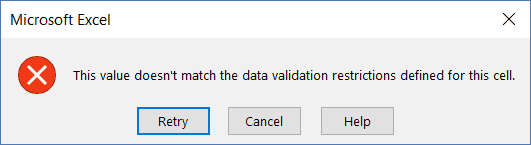
Now, if you use the data entry form to enter data in the Date column, and if it isn’t a date, then it will not be allowed.

You will see a message as shown below:

Similarly, you can use data validation with data entry forms to make sure users don’t end up entering the wrong data. Some examples where you can use this is numbers, text length, dates, etc.

Here are a few important things to know about Excel Data Entry Form:

You can use wildcard characters while navigating through the records (through criteria option).
You need to have an Excel table to be able to use the Data Entry Form. Also, you need to have a cell selected in it to use the form. There is one exception to this though. If you have a named range with the name ‘Database’, then the Excel Form will also refer to this named range, even if you have an Excel table.
The field width in the Data Entry form is dependent on the column width of the data. If your column width is too narrow, the same would be reflected in the form.
You can also insert bullet points in the data entry form. To do this, use the keyboard shortcut ALT + 7 or ALT + 9 from your numeric keypad. Here is a video about bullet points.

You May Also Like the Following Excel Tutorials:

Источник

Abstract: This is the first tutorial in a series designed to get you acquainted and comfortable using Excel and its built-in data mash-up and analysis features. These tutorials build and refine an Excel workbook from scratch, build a data model, then create amazing interactive reports using Power View. The tutorials are designed to demonstrate Microsoft Business Intelligence features and capabilities in Excel, PivotTables, Power Pivot, and Power View.

Note: This article describes data models in Excel 2013. However, the same data modeling and Power Pivot features introduced in Excel 2013 also apply to Excel 2016.

In these tutorials you learn how to import and explore data in Excel, build and refine a data model using Power Pivot, and create interactive reports with Power View that you can publish, protect, and share.

The tutorials in this series are the following:

Import Data into Excel 2013, and Create a Data Model
Extend Data Model relationships using Excel, Power Pivot, and DAX
Create Map-based Power View Reports
Incorporate Internet Data, and Set Power View Report Defaults
Power Pivot Help
Create Amazing Power View Reports — Part 2

In this tutorial, you start with a blank Excel workbook.

The sections in this tutorial are the following:

Import data from a database
Import data from a spreadsheet
Import data using copy and paste
Create a relationship between imported data
Checkpoint and Quiz

At the end of this tutorial is a quiz you can take to test your learning.

This tutorial series uses data describing Olympic Medals, hosting countries, and various Olympic sporting events. We suggest you go through each tutorial in order. Also, tutorials use Excel 2013 with Power Pivot enabled. For more information on Excel 2013, click here. For guidance on enabling Power Pivot, click here.

Import data from a database

We start this tutorial with a blank workbook. The goal in this section is to connect to an external data source, and import that data into Excel for further analysis.

Let’s start by downloading some data from the Internet. The data describes Olympic Medals, and is a Microsoft Access database.

Click the following links to download files we use during this tutorial series. Download each of the four files to a location that’s easily accessible, such as Downloads or My Documents, or to a new folder you create:
> OlympicMedals.accdb Access database
> OlympicSports.xlsx Excel workbook
> Population.xlsx Excel workbook
> DiscImage_table.xlsx Excel workbook
In Excel 2013, open a blank workbook.
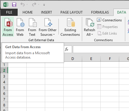
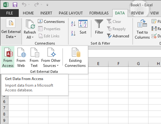
Click DATA > Get External Data > From Access. The ribbon adjusts dynamically based on the width of your workbook, so the commands on your ribbon may look slightly different from the following screens. The first screen shows the ribbon when a workbook is wide, the second image shows a workbook that has been resized to take up only a portion of the screen.
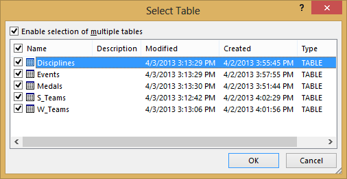
Select the OlympicMedals.accdb file you downloaded and click Open. The following Select Table window appears, displaying the tables found in the database. Tables in a database are similar to worksheets or tables in Excel. Check the Enable selection of multiple tables box, and select all the tables. Then click OK.
The Import Data window appears.

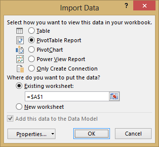
Note: Notice the checkbox at the bottom of the window that allows you to Add this data to the Data Model, shown in the following screen. A Data Model is created automatically when you import or work with two or more tables simultaneously. A Data Model integrates the tables, enabling extensive analysis using PivotTables, Power Pivot, and Power View. When you import tables from a database, the existing database relationships between those tables is used to create the Data Model in Excel. The Data Model is transparent in Excel, but you can view and modify it directly using the Power Pivot add-in. The Data Model is discussed in more detail later in this tutorial.

Select the PivotTable Report option, which imports the tables into Excel and prepares a PivotTable for analyzing the imported tables, and click OK.
Once the data is imported, a PivotTable is created using the imported tables.

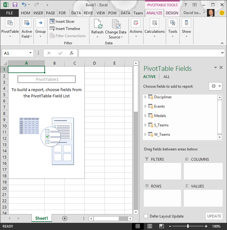
With the data imported into Excel, and the Data Model automatically created, you’re ready to explore the data.

Explore data using a PivotTable

Exploring imported data is easy using a PivotTable. In a PivotTable, you drag fields (similar to columns in Excel) from tables (like the tables you just imported from the Access database) into different areas of the PivotTable to adjust how it presents your data. A PivotTable has four areas: FILTERS, COLUMNS, ROWS, and VALUES.

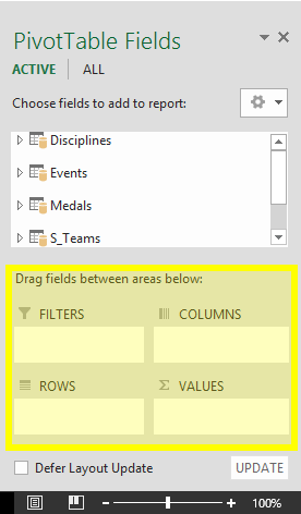
It might take some experimenting to determine which area a field should be dragged to. You can drag as many or few fields from your tables as you like, until the PivotTable presents your data how you want to see it. Feel free to explore by dragging fields into different areas of the PivotTable; the underlying data is not affected when you arrange fields in a PivotTable.

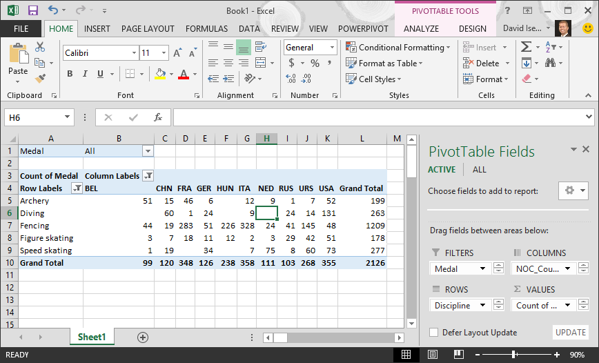
Let’s explore the Olympic Medals data in the PivotTable, starting with Olympic medalists organized by discipline, medal type, and the athlete’s country or region.

In PivotTable Fields, expand the Medals table by clicking the arrow beside it. Find the NOC_CountryRegion field in the expanded Medals table, and drag it to the COLUMNS area. NOC stands for National Olympic Committees, which is the organizational unit for a country or region.
Next, from the Disciplines table, drag Discipline to the ROWS area.
Let’s filter Disciplines to display only five sports: Archery, Diving, Fencing, Figure Skating, and Speed Skating. You can do this from within the PivotTable Fields area, or from the Row Labels filter in the PivotTable itself.
1. Click anywhere in the PivotTable to ensure the Excel PivotTable is selected. In the PivotTable Fields list, where the Disciplines table is expanded, hover over its Discipline field and a dropdown arrow appears to the right of the field. Click the dropdown, click (Select All)to remove all selections, then scroll down and select Archery, Diving, Fencing, Figure Skating, and Speed Skating. Click OK.
2. Or, in the Row Labels section of the PivotTable, click the dropdown next to Row Labels in the PivotTable, click (Select All) to remove all selections, then scroll down and select Archery, Diving, Fencing, Figure Skating, and Speed Skating. Click OK.
In PivotTable Fields, from the Medals table, drag Medal to the VALUES area. Since Values must be numeric, Excel automatically changes Medal to Count of Medal.
From the Medals table, select Medal again and drag it into the FILTERS area.
Let’s filter the PivotTable to display only those countries or regions with more than 90 total medals. Here’s how.
1. In the PivotTable, click the dropdown to the right of Column Labels.
2. Select Value Filters and select Greater Than….
3. Type 90 in the last field (on the right). Click OK.

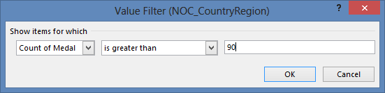
Your PivotTable looks like the following screen.

With little effort, you now have a basic PivotTable that includes fields from three different tables. What made this task so simple were the pre-existing relationships among the tables. Because table relationships existed in the source database, and because you imported all the tables in a single operation, Excel could recreate those table relationships in its Data Model.

But what if your data originates from different sources, or is imported at a later time? Typically, you can create relationships with new data based on matching columns. In the next step, you import additional tables, and learn how to create new relationships.

Import data from a spreadsheet

Now let’s import data from another source, this time from an existing workbook, then specify the relationships between our existing data and the new data. Relationships let you analyze collections of data in Excel, and create interesting and immersive visualizations from the data you import.

Let’s start by creating a blank worksheet, then import data from an Excel workbook.

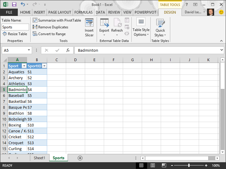
Insert a new Excel worksheet, and name it Sports.
Browse to the folder that contains the downloaded sample data files, and open OlympicSports.xlsx.
Select and copy the data in Sheet1. If you select a cell with data, such as cell A1, you can press Ctrl + A to select all adjacent data. Close the OlympicSports.xlsx workbook.
On the Sports worksheet, place your cursor in cell A1 and paste the data.
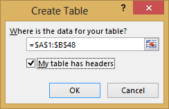
With the data still highlighted, press Ctrl + T to format the data as a table. You can also format the data as a table from the ribbon by selecting HOME > Format as Table. Since the data has headers, select My table has headers in the Create Table window that appears, as shown here.

Formatting the data as a table has many advantages. You can assign a name to a table, which makes it easy to identify. You can also establish relationships between tables, enabling exploration and analysis in PivotTables, Power Pivot, and Power View.
Name the table. In TABLE TOOLS > DESIGN > Properties, locate the Table Name field and type Sports. The workbook looks like the following screen.
Save the workbook.

Import data using copy and paste

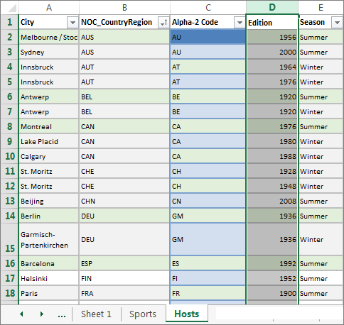
Now that we’ve imported data from an Excel workbook, let’s import data from a table we find on a web page, or any other source from which we can copy and paste into Excel. In the following steps, you add the Olympic host cities from a table.

Insert a new Excel worksheet, and name it Hosts.
Select and copy the following table, including the table headers.

City	NOC_CountryRegion	Alpha-2 Code	Edition	Season
Melbourne / Stockholm	AUS	AS	1956	Summer
Sydney	AUS	AS	2000	Summer
Innsbruck	AUT	AT	1964	Winter
Innsbruck	AUT	AT	1976	Winter
Antwerp	BEL	BE	1920	Summer
Antwerp	BEL	BE	1920	Winter
Montreal	CAN	CA	1976	Summer
Lake Placid	CAN	CA	1980	Winter
Calgary	CAN	CA	1988	Winter
St. Moritz	SUI	SZ	1928	Winter
St. Moritz	SUI	SZ	1948	Winter
Beijing	CHN	CH	2008	Summer
Berlin	GER	GM	1936	Summer
Garmisch-Partenkirchen	GER	GM	1936	Winter
Barcelona	ESP	SP	1992	Summer
Helsinki	FIN	FI	1952	Summer
Paris	FRA	FR	1900	Summer
Paris	FRA	FR	1924	Summer
Chamonix	FRA	FR	1924	Winter
Grenoble	FRA	FR	1968	Winter
Albertville	FRA	FR	1992	Winter
London	GBR	UK	1908	Summer
London	GBR	UK	1908	Winter
London	GBR	UK	1948	Summer
Munich	GER	DE	1972	Summer
Athens	GRC	GR	2004	Summer
Cortina d’Ampezzo	ITA	IT	1956	Winter
Rome	ITA	IT	1960	Summer
Turin	ITA	IT	2006	Winter
Tokyo	JPN	JA	1964	Summer
Sapporo	JPN	JA	1972	Winter
Nagano	JPN	JA	1998	Winter
Seoul	KOR	KS	1988	Summer
Mexico	MEX	MX	1968	Summer
Amsterdam	NED	NL	1928	Summer
Oslo	NOR	NO	1952	Winter
Lillehammer	NOR	NO	1994	Winter
Stockholm	SWE	SW	1912	Summer
St Louis	USA	US	1904	Summer
Los Angeles	USA	US	1932	Summer
Lake Placid	USA	US	1932	Winter
Squaw Valley	USA	US	1960	Winter
Moscow	URS	RU	1980	Summer
Los Angeles	USA	US	1984	Summer
Atlanta	USA	US	1996	Summer
Salt Lake City	USA	US	2002	Winter
Sarajevo	YUG	YU	1984	Winter

In Excel, place your cursor in cell A1 of the Hosts worksheet and paste the data.
Format the data as a table. As described earlier in this tutorial, you press Ctrl + T to format the data as a table, or from HOME > Format as Table. Since the data has headers, select My table has headers in the Create Table window that appears.
Name the table. In TABLE TOOLS > DESIGN > Properties locate the Table Name field, and type Hosts.
Select the Edition column, and from the HOME tab, format it as Number with 0 decimal places.
Save the workbook. Your workbook looks like the following screen.

Now that you have an Excel workbook with tables, you can create relationships between them. Creating relationships between tables lets you mash up the data from the two tables.

Create a relationship between imported data

You can immediately begin using fields in your PivotTable from the imported tables. If Excel can’t determine how to incorporate a field into the PivotTable, a relationship must be established with the existing Data Model. In the following steps, you learn how to create a relationship between data you imported from different sources.

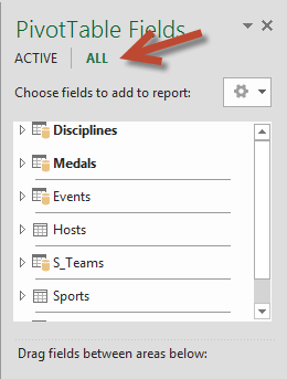
On Sheet1, at the top ofPivotTable Fields, clickAll to view the complete list of available tables, as shown in the following screen.
Scroll through the list to see the new tables you just added.
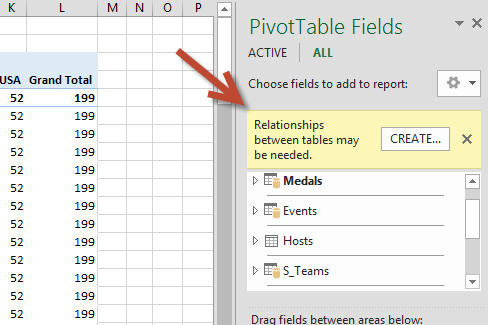
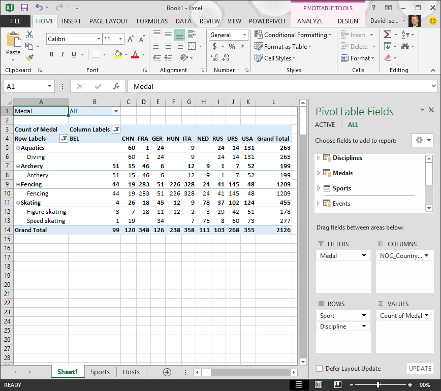
Expand Sports and select Sport to add it to the PivotTable. Notice that Excel prompts you to create a relationship, as seen in the following screen.

This notification occurs because you used fields from a table that’s not part of the underlying Data Model. One way to add a table to the Data Model is to create a relationship to a table that’s already in the Data Model. To create the relationship, one of the tables must have a column of unique, non-repeated, values. In the sample data, the Disciplines table imported from the database contains a field with sports codes, called SportID. Those same sports codes are present as a field in the Excel data we imported. Let’s create the relationship.
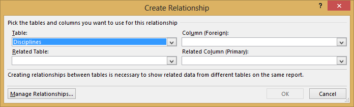
Click CREATE… in the highlighted PivotTable Fields area to open the Create Relationship dialog, as shown in the following screen.
In Table, choose Disciplines from the drop down list.
In Column (Foreign), choose SportID.
In Related Table, choose Sports.
In Related Column (Primary), choose SportID.
Click OK.

The PivotTable changes to reflect the new relationship. But the PivotTable doesn’t look right quite yet, because of the ordering of fields in the ROWS area. Discipline is a subcategory of a given sport, but since we arranged Discipline above Sport in the ROWS area, it’s not organized properly. The following screen shows this unwanted ordering.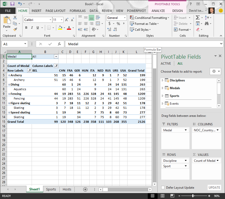

In the ROWS area, move Sport above Discipline. That’s much better, and the PivotTable displays the data how you want to see it, as shown in the following screen.

Behind the scenes, Excel is building a Data Model that can be used throughout the workbook, in any PivotTable, PivotChart, in Power Pivot, or any Power View report. Table relationships are the basis of a Data Model, and what determine navigation and calculation paths.

In the next tutorial, Extend Data Model relationships using Excel 2013, Power Pivot, and DAX, you build on what you learned here, and step through extending the Data Model using a powerful and visual Excel add-in called Power Pivot. You also learn how to calculate columns in a table, and use that calculated column so that an otherwise unrelated table can be added to your Data Model.

Checkpoint and Quiz

Review What You’ve Learned

You now have an Excel workbook that includes a PivotTable accessing data in multiple tables, several of which you imported separately. You learned to import from a database, from another Excel workbook, and from copying data and pasting it into Excel.

To make the data work together, you had to create a table relationship that Excel used to correlate the rows. You also learned that having columns in one table that correlate to data in another table is essential for creating relationships, and for looking up related rows.

You’re ready for the next tutorial in this series. Here’s a link:

Extend Data Model relationships using Excel 2013, Power Pivot, and DAX

QUIZ

Want to see how well you remember what you learned? Here’s your chance. The following quiz highlights features, capabilities, or requirements you learned about in this tutorial. At the bottom of the page, you’ll find the answers. Good luck!

Question 1: Why is it important to convert imported data into tables?

A: You don’t have to convert them into tables, because all imported data is automatically turned into tables.

B: If you convert imported data into tables, they will be excluded from the Data Model. Only when they’re excluded from the Data Model are they available in PivotTables, Power Pivot, and Power View.

C: If you convert imported data into tables, they can be included in the Data Model, and be made available to PivotTables, Power Pivot, and Power View.

D: You cannot convert imported data into tables.

Question 2: Which of the following data sources can you import into Excel, and include in the Data Model?

A: Access Databases, and many other databases as well.

B: Existing Excel files.

C: Anything you can copy and paste into Excel and format as a table, including data tables in websites, documents, or anything else that can be pasted into Excel.

D: All of the above

Question 3: In a PivotTable, what happens when you reorder fields in the four PivotTable Fields areas?

A: Nothing – you cannot reorder fields once you place them in the PivotTable Fields areas.

B: The PivotTable format is changed to reflect the layout, but underlying data is unaffected.

C: The PivotTable format is changed to reflect the layout, and all underlying data is permanently changed.

D: The underlying data is changed, resulting in new data sets.

Question 4: When creating a relationship between tables, what is required?

A: Neither table can have any column that contains unique, non-repeated values.

B: One table must not be part of the Excel workbook.

C: The columns must not be converted to tables.

D: None of the above is correct.

Quiz Answers

Correct answer: C
Correct answer: D
Correct answer: B
Correct answer: D

Notes: Data and images in this tutorial series are based on the following:

Olympics Dataset from Guardian News & Media Ltd.
Flag images from CIA Factbook (cia.gov)
Population data from The World Bank (worldbank.org)
Olympic Sport Pictograms by Thadius856 and Parutakupiu

Источник

Data entry can sometimes be a big part of using Excel.

With near endless cells, it can be hard for the person inputting data to know where to put what data.

A data entry form can solve this problem and help guide the user to input the correct data in the correct place.

Excel has had VBA user forms for a long time, but they are complicated to set up and not very flexible to change.

In this blog post, we’re going to explore 5 easy ways to create a data entry form for Excel.

Video Tutorial

Excel Tables

We’ve had Excel tables since Excel 2007.

They’re perfect data containers and can be used as a simple data entry form.

Creating a table is easy.

Select the range of data including the column headings.
Go to the Insert tab in the ribbon.
Press the Table button in the Tables section.

We can also use a keyboard shortcut to create a table. The Ctrl + T keyboard shortcut will do the same thing.

Make sure the Create Table dialog box has the My table has headers option checked and press the OK button.

We now have our data inside an Excel table and we can use this to enter new data.

To add new data into our table we can start typing a new entry into the cells directly below the table and the table will absorb the new data.

We can use the Tab key instead of Enter while entering our data. This will cause the active cell cursor to move to the right instead of down so we can add the next value into our record.

When the active cell cursor is in the last cell of the table (lower right cell), pressing the Tab key will create a new empty row in the table ready for the next entry.

This is a perfect and simple data entry form.

Data Entry Form

Excel actually has a hidden data entry form and we can access it by adding the command to the Quick Access Toolbar.

Add the form command to the Quick Access Toolbar.

Right click anywhere on the quick quick access toolbar.
Select Customize Quick Access Toolbar from the menu options.

This will open up the Excel option menu on the Quick Access Toolbar tab.

Select Commands Not in the Ribbon.
Select Form from the list of available commands. Press F to jump to the commands starting with F.
Press the Add button to add the command into the quick access toolbar.
Press the OK button.

We can then open up data entry form for any set of data.

Select a cell inside the data which we want to create a data entry form with.
Click on the Form icon in the quick access toolbar area.

This will open up a customized data entry form based on the fields in our data.

Microsoft Forms

If we need a simple data entry form, why not use Microsoft Forms?

This form option will require our Excel workbook to be saved into SharePoint or OneDrive.

The form will be in a browser and not in Excel, but we can link the form to an Excel workbook so that all the data goes into our Excel table.

This is a great option if multiple people or people outside our organization need to input data into the Excel workbook.

We need to create a Form for Excel in either SharePoint or OneDrive. The process is the same for both SharePoint or OneDrive.

Go to a SharePoint document library or a OneDrive folder where the Excel workbook is going to be saved.
Click on New and then choose Forms for Excel.

This will prompt us to name the Excel workbook and open up a new browser tab where we can build our form by adding different types of questions.

We first need to create the Form and this will create the table in our Excel workbook where the data will get populated.

Then we can share the form with anyone we want to input data into Excel.

When a user enters data into the form and presses the submit button, that data will automatically show up into our Excel workbook.

Power Apps

Power Apps is a flexible drag and drop formula based app building platform from Microsoft.

We can certainly use it to create a data entry from for our Excel data.

In fact, if we have a table of data set up, Power Apps will create the app for us based on our data. It can’t be any easier than that.

Sign in to the powerapps.microsoft.com service ➜ go to the Create tab in the navigation pane ➜ select Excel Online.

We’ll then be prompted to sign in to our SharePoint or OneDrive account where our Excel file is saved to select the Excel workbook and table with our data.

This will generate us a fully functional three screen data entry app.

We can search and view all the records in our Excel table in a scroll-able gallery.
We can view an individual record in our data.
We can edit an existing record or add new records.

This is all connected to our Excel table, so any changes or additions from the app will show up in Excel.

Power Automate

Power Automate is a cloud based tool for automating task between apps.

But we can use the button trigger to make an automation that captures user input and adds the data into an Excel table.

We’ll need to have our Excel workbook saved in OneDrive or SharePoint and have a table already setup with the fields we want to populate.

To create our Power Automate data entry form.

Go to flow.microsoft.com and sign in.
Go to the Create tab.
Create an Instant flow.
Give the flow a name.
Choose the Manually trigger a flow option as the trigger.
Press the Create button.

This will open up the Power Automate builder and we can build our automation.

Click on the Manually trigger a flow block to expand the trigger’s options. This is where we’ll find the ability to add input fields.
Click on the Add an input button. This will give us options to add a few different types of input fields including Text, Yes/No, Files, Email, Number and Dates.
Rename the field to something descriptive. This will help the user know what type of data to input when they run this automation.
Click on the three ellipses to the right of each field to change the input options. We’ll be able to Add a drop-down list of option, Add a multi-select list of options, Make the field optional or Delete the field from this menu.
After we have added all our input fields, we can now add a New step to the automation.

Search for the Excel connector and add the Add a row into a table action. If you’re on an Office 365 business account, use the Excel Online (Business) connectors, otherwise use the Excel Online (OneDrive) connectors.

Now we can set up our Excel Add a row into a table step.

Navigate to the Excel file and table where we are going to be adding data.
After selecting the table, the fields in that table will appear listed and we can add the appropriate dynamic content from the Manually trigger a flow trigger step.

Now we can run our Flow from the Power Automate service.

Go to My flows in the left navigation pane.
Go to the My flows tab.
Find the flow in the list of available flows and click on the Run button.
A side pane will pop up with our inputs and we can enter our data.
Click Run flow.

We can also run this from our mobile device with the Power Automate apps.

Go to the Buttons section in the app.
Press on the flow to run.
Enter the data inputs in the form.
Press on the DONE button in the top right.

Whichever way we run the flow, a few seconds later the data will appear in our Excel table.

Conclusions

Whether we require a simple form or something more complex and customize-able, there is a solution for our data entry needs.

We can quickly create something inside our workbook or use an external solution that connects to and loads data into Excel.

We can even create forms that people outside our organization can use to populate our spreadsheets.

Let me know in the comments what is your favourite data entry form option.

About the Author

John MacDougall

John is a Microsoft MVP and qualified actuary with over 15 years of experience. He has worked in a variety of industries, including insurance, ad tech, and most recently Power Platform consulting. He is a keen problem solver and has a passion for using technology to make businesses more efficient.

Источник

Data Entry Forms is an extremely useful feature if inputting data is part of your daily work.

It can help you avoid the mistakes and make the data entry process faster. It also helps you focus on one record at a time!

It is a convenient and faster way to input records in Excel by displaying one row of information at a time without having to move from one column to another.

In this tutorial, we will show you How to Create Form in Excel for Data Entry.

Whenever I wanted to enter data in Excel, it would take me a very long time to input these records one by one, but I discovered a handy trick that can turn my Excel Table into a handy Excel Data Entry Form!

Say goodbye to inputting entering data into this Table row by row by row by row….

Below, we will cover the Top 11 Excel Data Entry Form Tips and Tricks that will be beneficial for you:

#1 – Create Form in Excel
#2 – Add to Quick Access Toolbar (QAT)
#3 – Access the Form anytime
#4 – Browse through Records
#5 – Edit Existing Record
#6 – Search Criteria
#7 – Restore a Record
#8 – Data Validation in Forms
#9 – Delete a Record
#10 – Close the Form
#11 – Keyboard Shortcuts for Data Entry Forms

Make sure to download the Excel Workbook below and follow along:

DOWNLOAD EXCEL WORKBOOK

Want to know how to use the Data Entry Form?

*** Watch our video and step by step guide below with free downloadable Excel workbook to practice ***

Watch it on YouTube and give it a thumbs-up!

1. Create Form in Excel

I will show you how easy it is to Create Form in Excel for Data Entry with the following quick video below (scroll further down to see the step by step instructions after you watch this awesome video).

*** Watch our video below on How to Create Form in Excel in 5 minutes!***

DOWNLOAD OUR
FREE EXCEL GUIDES

In this tutorial, you have learned how to create form in Excel with minutes without using VBA!!

Follow the steps below:

STEP 1: Convert your Column names into a Table, go to Insert> Table

Make sure My table has headers is also checked.

STEP 2:Let us add the Form Creation functionality to understand how to make a fillable form in Excel.

Go to File > Options

STEP 3:Go to Customize Ribbon.

Select Commands Not in the Ribbon and Form. This is the functionality we need.

Click New Tab.

STEP 4:Under the New Tab, select New Group, and click Add.

This will add Forms to a New Tab in our Ribbon.

Notice that there is also a Rename button, you can use it to rename the New Tab and New Group into something more descriptive, like Form:

STEP 5:Select your Table, and on your new Form tab, select Form.

STEP 6: A new Form dialogue box will pop up!

Input your data into each section.

Click New to save it. Repeat this process for all the records you want to add.

Press Close to get out of this screen and see the data in your Excel Table.

You can now use this new form to continually input data into your Excel Table!

2. Add to Quick Access Toolbar (QAT)

Now that you have learned how to create form in Excel, lets put them on your QAT for easy access.

To add to the quick access toolbar, follow the steps below:

STEP 1: Click on the small arrow right next to QAT.

STEP 2: Click on More Commands from the dropdown list.

STEP 3: In the Excel Options dialog box, select All Commands from Choose commands from list.

STEP 4: Select Form from the list and then click on Add>>.

STEP 5: Form is now available in the Customize Quick Access Toolbar. Click OK.

Data Entry Form is now part of your Quick Access Toolbar.

3. Access the Form anytime

To access the Excel Data Entry Form, click on any cell in the table and click on the Form icon in Quick Access Toolbar.

If you try to access the form when you haven’t selected a cell within the data table, you will receive an error message like the one shown below:

4. Browse through Records

To navigate through the existing records, simply use the Find Previous and Find Next buttons available on the Data Entry Form.

You can also use the scroll bar to go through the records one after the other.

This will save time when you have a data with multiple columns and records.

5. Edit Existing Record

Use the Find Previous and Find Next buttons to search for the record to want to edit.

Once you find the desired record, simply make the necessary edit and hit Enter in Excel.

The data table will be updated with the changes made.

6. Search Criteria

Using Wildcards

If you wish to search all entries containing the word “east” in the Region Column, you can do that by using the wildcard asterisk (*).

STEP 1: In the Data Entry Form, click on the Criteria button

STEP 2: In the Region field, type *east (to search all-region containing the word east)

STEP 3: Click Find Next to find the entries containing the word east.

Excel Data Entry Form will find the three entries for you in this scenario!

Using greater or less than sign

If you want to search for persons having a salary greater than or equal to $75,000, you can do so by following the steps below:

STEP 1: In the Data Entry Form, click on the Criteria button

STEP 2: In the Salary field, type >=75000.

STEP 3: Click Find Next to find all entries with a salary greater than or equal to $75,000.

7. Restore a Record

Suppose you have accidentally deleted the first name of a record.

And you don’t remember what was written in that field! Don’t panic.

You can use the Restore button in the Excel Data Entry Form and retrieve the data lost accidentally.

The data will reappear in the respective field.

One thing you need to keep in mind is that the Restore button is only useful if you haven’t hit Enter.

The moment you press the Enter button, the Restore button will become inactive and you won’t be able to revert back to the original data.

8. Data Validation in Forms

Even though you cannot directly add any data validation to the form. Any restriction created on the data table will still be in effect in the Forms.

Let’s see how!

Say, you add a list rule to the Region Column using Data Validation.

STEP 1: Select the Region Column.

STEP 2: Go to Data Tab > Data Tools (Group) > Data Validation.

STEP 3: In the Data Validation dialog box, click on the Allow dropdown and select List.

STEP 4: In the Source field, type Northeast, Northwest, Southeast, Southwest, and click OK.

Data Validation has now been inserted in the Region Column where you are only allowed to enter values present in the list (Northeast, Northwest, Southeast, Southwest).

STEP 5: Click on the Forms icon in QAT.

STEP 6: Change the Region for Record 1 from Northeast to East and Click OK.

Once you click OK, you will see an error message as below:

9. Delete a Record

STEP 1: Use the Scroll Bar to navigate to find the entry you want to delete.

STEP 2: Simply, click on the Delete button.

STEP 3: A confirmation message will appear on your screen, Click OK.

The desired entry will be removed from the data table.

10. Close the Form

To close the dialog box for Data Forms, simply click on the Close button (X) on the top-right corner of the bix.

11. Keyboards Shortcuts for Data Entry Forms

You can use the following keyboard shortcuts to work faster when using Data Entry Forms:

Press Tab to go to the next field in the Excel Forms.
Press Enter to go to the next record in the Excel Forms.
Hit the Esc button on your keyboard to close the Excel Form.

This completes our tutorial on the Top 11 things you should know if Data Entry is what you do in Excel. It will not only make the process faster but also a lot more easier and fun!

Few things to keep in mind when using the Excel Data Entry Form are:

You can add a maximum of 32 fields per record.
You cannot print a data form record.
Before you hit Enter, you can restore any changes made to the data.

So, give it a try! I am sure you are gonna love it!!

You can know more about How to Create Form in Excel by going through this tutorial by Microsoft.

Источник

Watch the Video on Using Data Entry Forms in Excel

Below is a detailed written tutorial about Excel Data Entry form in case you prefer reading over watching a video.

Excel has many useful features when it comes to data entry.

And one such feature is the Data Entry Form.

In this tutorial, I will show you what are data entry forms and how to create and use them in Excel.

Why Do You Need to Know About Data Entry Forms?

Maybe you don’t!

But if data entry is a part of your daily work, I recommend you check out this feature and see how it can help you save time (and make you more efficient).

There are two common issues that I have faced (and seen people face) when it comes to data entry in Excel:

It’s time-consuming. You need to enter the data in one cell, then go to the next cell and enter the data for it. Sometimes, you need to scroll up and see which column it is and what data needs to be entered. Or scroll to the right and then come back to the beginning in case there are many columns.
It’s error-prone. If you have a huge data set which needs 40 entries, there is a possibility you may end up entering something that was not intended for that cell.

A data entry form can help by making the process faster and less error-prone.

Before I show you how to create a data entry form in Excel, let me quickly show you what it does.

Below is a data set that is typically maintained by the hiring team in an organization.

Every time a user has to add a new record, he/she will have to select the cell in the next empty row and then go cell by cell to make the entry for each column.

While this is a perfectly fine way of doing it, a more efficient way would be to use a Data Entry Form in Excel.

Below is a data entry form that you can use to make entries to this data set.

The highlighted fields are where you would enter the data. Once done, hit the Enter key to make the data a part of the table and move on to the next entry.

Below is a demo of how it works:

As you can see, this is easier than regular data entry as it has everything in a single dialog box.

Data Entry Form in Excel

Using a data entry form in Excel needs a little pre-work.

You would notice that there is no option to use a data entry form in Excel (not in any tab in the ribbon).

To use it, you will have to first add it to the Quick Access Toolbar (or the ribbon).

Adding Data Entry Form Option To Quick Access Toolbar

Below are the steps to add the data entry form option to the Quick Access Toolbar:

Right-click on any of the existing icons in the Quick Access Toolbar.
Click on ‘Customize Quick Access Toolbar’.
In the ‘Excel Options’ dialog box that opens, select the ‘All Commands’ option from the drop-down.
Scroll down the list of commands and select ‘Form’.
Click on the ‘Add’ button.
Click OK.

The above steps would add the Form icon to the Quick Access Toolbar (as shown below).

Once you have it in QAT, you can click any cell in your dataset (in which you want to make the entry) and click on the Form icon.

Note: For Data Entry Form to work, your data should be in an Excel Table. If it isn’t already, you’ll have to convert it into an Excel Table (keyboard shortcut – Control + T).

Parts of the Data Entry Form

A Data Entry Form in Excel has many different buttons (as you can see below).

Here is a brief description of what each button is about:

New: This will clear any existing data in the form and allows you to create a new record.
Delete: This will allow you to delete an existing record. For example, if I hit the Delete key in the above example, it will delete the record for Mike Banes.
Restore: If you’re editing an existing entry, you can restore the previous data in the form (if you haven’t clicked New or hit Enter).
Find Prev: This will find the previous entry.
Find Next: This will find the next entry.
Criteria: This allows you to find specific records. For example, if I am looking for all the records, where the candidate was Hired, I need to click the Criteria button, enter ‘Hired’ in the Status field and then use the find buttons. Example of this is covered later in this tutorial.
Close: This will close the form.
Scroll Bar: You can use the scroll bar to go through the records.

Now let’s go through all the things you can do with a Data Entry form in Excel.

Note that you need to convert your data into an Excel Table and select any cell in the table to be able to open the Data Entry form dialog box.

If you haven’t selected a cell in the Excel Table, it will show a prompt as shown below:

Creating a New Entry

Below are the steps to create a new entry using the Data Entry Form in Excel:

Select any cell in the Excel Table.
Click on the Form icon in the Quick Access Toolbar.
Enter the data in the form fields.
Hit the Enter key (or click the New button) to enter the record in the table and get a blank form for next record.

Navigating Through Existing Records

One of the benefits of using Data Entry Form is that you can easily navigate and edit the records without ever leaving the dialog box.

This can be especially useful if you have a dataset with many columns. This can save you a lot of scrolling and the process of going back and forth.

Below are the steps to navigate and edit the records using a data entry form:

Select any cell in the Excel Table.
Click on the Form icon in the Quick Access Toolbar.
To go to the next entry, click on the ‘Find Next’ button and to go to the previous entry, click the ‘Find Prev’ button.
To edit an entry, simply make the change and hit enter. In case you want to revert to the original entry (if you haven’t hit the enter key), click the ‘Restore’ button.

You can also use the scroll bar to navigate through entries one-by-one.

The above snapshot shows basic navigation where you are going through all the records one after the other.

But you can also quickly navigate through all the records based on criteria.

For example, if you want to go through all the entries where the status is ‘In-progress’, you can do that using the below steps:

Criteria is a very useful feature when you have a huge dataset, and you want to quickly go through those records that meet a given set of criteria.

Note that you can use multiple criteria fields to navigate through the data.

You can also use wildcard characters in criteria.

Below are the steps to do this:

Select any cell in the Excel table.
Click on the Form icon in the Quick Access Toolbar.
Click the Criteria button.
In the Status field, enter *progress
Use the Find Prev/Find Next buttons to navigate through the entries where the status is In-Progress.

Deleting a Record

You can delete records from the Data Entry form itself.

This can be useful when you want to find a specific type of records and delete these.

Below are the steps to delete a record using Data Entry Form:

Select any cell in the Excel table.
Click on the Form icon in the Quick Access Toolbar.
Navigate to the record you want to delete
Click the Delete button.

Restricting Data Entry Based on Rules

You can use data validation in cells to make sure the data entered conforms to a few rules.

For example, if you want to make sure that the date column only accepts a date during data entry, you can create a data validation rule to only allow dates.

If a user enters a data that is not a date, it will not be allowed and the user will be shown an error.

Here is how to create these rules when doing data entry:

Select the cells (or even the entire column) where you want to create a data validation rule. In this example, I have selected column A.
Click the Data tab.
Click the Data Validation option.
In the ‘Data Validation’ dialog box, within the ‘Settings’ tab, select ‘Date’ from the ‘Allow’ drop down.
Specify the start and the end date. Entries within this date range would be valid and rest all would be denied.
Click OK.

Now, if you use the data entry form to enter data in the Date column, and if it isn’t a date, then it will not be allowed.

You will see a message as shown below:

Similarly, you can use data validation with data entry forms to make sure users don’t end up entering the wrong data. Some examples where you can use this is numbers, text length, dates, etc.

Here are a few important things to know about Excel Data Entry Form:

You can use wildcard characters while navigating through the records (through criteria option).
You need to have an Excel table to be able to use the Data Entry Form. Also, you need to have a cell selected in it to use the form. There is one exception to this though. If you have a named range with the name ‘Database’, then the Excel Form will also refer to this named range, even if you have an Excel table.
The field width in the Data Entry form is dependent on the column width of the data. If your column width is too narrow, the same would be reflected in the form.
You can also insert bullet points in the data entry form. To do this, use the keyboard shortcut ALT + 7 or ALT + 9 from your numeric keypad. Here is a video about bullet points.

You May Also Like the Following Excel Tutorials:

100+ Excel Interview Questions.
Drop Down Lists in Excel.
Find and Remove Duplicates in Excel.
Excel Text to Columns.

Источник