

We all deal with multiple sheets in a single workbook, don’t we? Here is a smart way to create an Index of all your Sheets. You can click on the sheet name to navigate to that sheet.
Here is how we do it
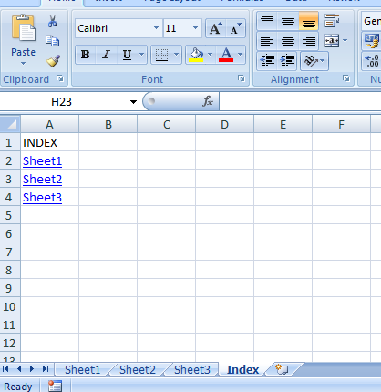
Assume that we have 5 Sheets
![]()
And we would like to have an Index placed (in a new sheet) with the sheet names hyperlinked to the respective sheet.
It can be done with a simple VBA Code
Here comes a Code
Sub CreateIndex()
Dim sheetnum As Integer
Sheets.Add before:=Sheets(1)
For sheetnum = 2 To Worksheets.Count
 ActiveSheet.Hyperlinks.Add _
 Anchor:=Cells(sheetnum - 1, 1), _
 Address:='', _
 SubAddress:=''' & Worksheets(sheetnum).Name & ''!A1', _
 TextToDisplay:=Worksheets(sheetnum).Name
Next sheetnum
ActiveWindow.DisplayGridlines = False
End Sub
Follow the steps
- Copy this Code
- Open the excel workbook where you want to create a Sheet Index
- Press the shortcut Alt + F11 to open the Visual Basic Window
- In the Insert Menu, click on Module or use the shortcut Alt i m to add a Module. Module is the place where the code is written
- In the blank module paste the code and close the Visual Basic Editor
- Then use the shortcut Alt + F8 to open the Macro Box. You would have the list of all the macros here
- You would see the Macro that you have just pasted in the Module as ‘CreateIndex’
- Run it. You would see an Index with all the sheet names hyperlinked to the respective sheet.
Other Useful Macros
- Automated Filter with Macro
- Unhiding Multiple Sheets at Once
- Covert Numbers into Indian Currency Words
Topics that I write about…

goodly
Do you want one central location where you can easily navigate to any worksheet in your file, and then navigate back with one click? This macro lets you quickly and easily create an index in Excel that lists all sheets in your workbook. The best part is that the index excel macro updates itself every time you select the index sheet! Indexing in Excel made simple.
If you need an index sheet in your file, you probably already have a zillion worksheets in your file, here is how to make an index in Excel
- Add a tab and call it “Index” or whatever you want to identify it as an index (table of contents, etc.).
- Right click the Index tab and select ‘View Code’.
- Enter the VBA code below. Click on another sheet in your file, then click back on your Index sheet. Hey presto! you’ll notice that it has populated a list of all the sheets in your file, complete with a convenient link to them.
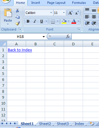
In all your other sheets, cell A1 will have a “Back to Index” link for easy navigation. If you want to use another cell for this backwards navigation, change the code in both places where it says A1 to whatever cell you’d like. Here is what your index in Excel will look like when done.
Need help? Use our nifty guide to help figure out how to install and use your macros.
Private Sub Worksheet_Activate()

'

'MACROS BY EXCELZOOM.COM - create index in excel

'

Dim wSheet As Worksheet

Dim l As Long

l = 1

With Me

.Columns(1).ClearContents

.Cells(1, 1) = "INDEX"

.Cells(1, 1).Name = "Index"

End With

For Each wSheet In Worksheets

If wSheet.Name <> Me.Name Then

l = l + 1

With wSheet

.Range("A1").Name = "Start_" & wSheet.Index

.Hyperlinks.Add Anchor:=.Range("A1"), Address:="", _

SubAddress:="Index", TextToDisplay:="Back to Index"

End With

Me.Hyperlinks.Add Anchor:=Me.Cells(l, 1), Address:="", _

SubAddress:="Start_" & wSheet.Index, TextToDisplay:=wSheet.Name

End If

Next wSheet

End Sub
We hope this how to index in excel guide helps making an index in excel painless and easy for you. We love this macro code and have opted to make it available to all free of any charge and unrestricted from our members area so you can enjoy the wizardry of this auto updating index in excel  Find that tab in excel with your new Index Sheet and impress all your colleagues in the process..
Have some comments about indexing in Excel, we would love to hear them
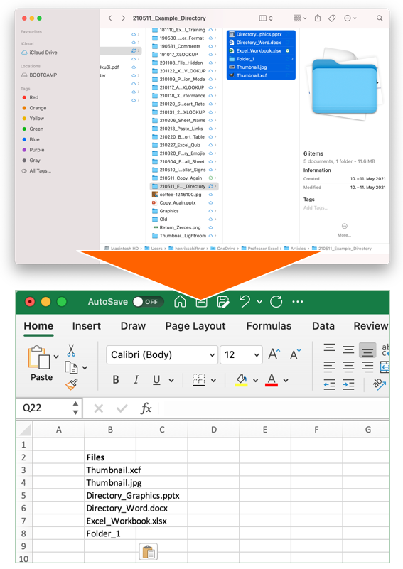
You probably don’t need this every day: But once a file you might want to have a list of all files within a folder or directory in Excel. The good thing: There are many methods available. If you Google it, you will find a lot of different methods to create a file list in Excel. But unfortunately, all of them have advantages and disadvantages – which you usually only find out after trying them. That’s the reason for this article: You won’t only learn each method step by step: You will rather find an overview comparing all the advantages and disadvantages of each method. After seeing this, you don’t need to start extensive trials and errors. Much better: You can easily select the method that works best for you!
Summary
| Method 1: Copy & Paste on Mac |
Method 2: Named function |
Method 3: Internet browser |
Method 4: PowerQuery |
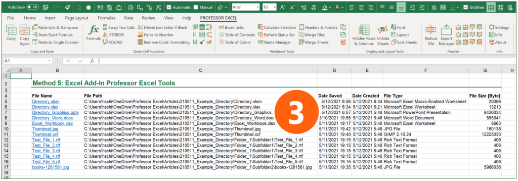
Method 5: Excel-Add-In |
Method 6: Windows PowerShell |
Method 7: VBA Macro |
|
|---|---|---|---|---|---|---|---|
| Short description | Copy and paste from the Mac Finder. | Use a function in a named range to insert a file list. | Open folder with a web browser and copy the file list. | Use PowerQuery to insert a directory. | Let an Excel add-in do the work for you. | Use the Windows built-in PowerShell feature. | Use a VBA Macro to insert a file list. |
| Ease of use |  |
|
|
|
|
|
|
| Operating system | Mac | Windows | Windows / Mac | Windows / Mac | Windows | Windows | Windows |
| Include subfolders and files |
No | No | No | Yes | Yes | Yes | (Yes) (depends on the VBA macro) |
| File information available | File names | File names | File names, file links (not working properly), file size, date modified | Folder path, name extension, date accessed, date modified, date created More attributes: Content type, kind, size, ReadOnly, hidden, S |
Links to files on the drive, file path, date and time last saved, date and time created, file size, file type | File name, file path, date and time last saved, file size | Depends on the VBA macro |
| Technology | Mac Finder | Named function in Excel | Internet browser | PowerQuery | Excel Add-In | PowerShell, Text Import Wizard | VBA |
| Comment | Fast but with limited options. | Only shows files, no folders. | File links not working in our test; not working with all internet browsers (tested with Google Chrome and working). | Elegant and uses built-in functions. | Convenient, fast and many options. | Results not good, difficult process; performs well on large file structures, though. | Modifying the macro rather for advanced users. |
| Link | Click here | Click here | Click here | Click here | Click here | Click here | Click here |
Method 1: Simply copy and paste from Mac Finder to Excel
This first method works on a Mac only: Just select all files in a Finder window and press copy (Command + C on the keyboard). Next, switch to Excel and paste the list: Press Command + V on the keyboard.
The advantage of this method is that it’s very easy and fast. Unfortunately, you don’t have any further options than just pasting the file names. That means you can’t insert data of subfolders or file properties.
Recommendation: Use this if you need a quick file list on the Mac – without any further information.
Method 2: Insert a file list with built-in Excel functions using “Named Ranges”
The second method is actually quite elegant: Use built-in Excel functions to insert a file list in Excel. It is built on advanced functions, such as an Excel function within a named range. But following these steps should be quite straight-forward.
Set up the named range
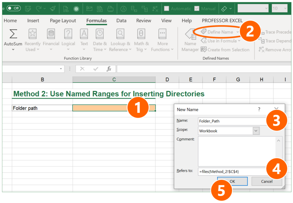
- Choose a cell in which you later write the folder path. In this case, it’s cell C4.
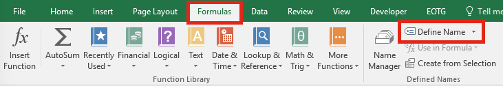
- Click on “Defined Name” on the Formulas ribbon.
- Give a name for the cell containing the folder path (here: “Folder_Path”)
- In the “Refers to” field, type: =files(linktopathcell) (replace “linktopathcell” with your cell reference – in this case “Method_2!$C$4”).
- Confirm with OK.
Use the named range in Excel functions
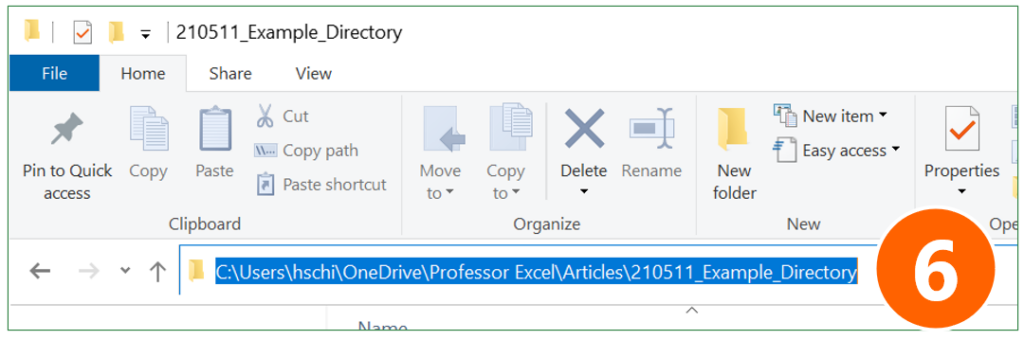
- Go to the Windows Explorer and copy the folder path.
- Paste the folder link into the folder path cell (the cell you have set as the named range in step 1 above). Add one of the following endings:
- If you want to include all files – no matter which file type – in your list, add *
- For listing only Excel files, add *.xls*
- If you want to see all files ending on “.xlsx”, add *.xlsx
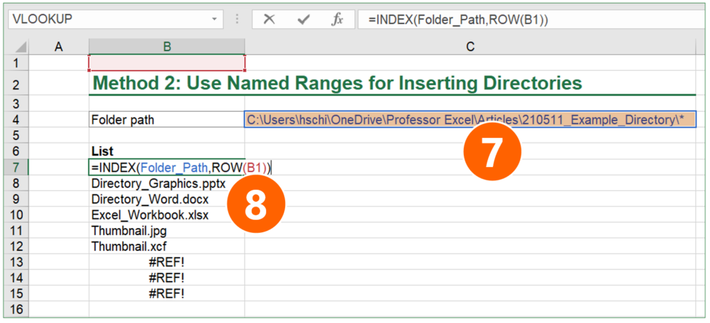
- As the last step, enter an INDEX function for compiling the list (here in cell B7):
=INDEX(Folder_Path,ROW(B1))
Folder_Path should be the same name that you have given in step 3 above. The ROW function should refer to any cell in the first row (for example to B1). That means, this argument could also be A1, C1, etc.
As the last step: Copy the INDEX function down until you see the first #REF error. #REF means in this case that there are no more files in your folder. If you like, you could wrap the IFERROR function around in order to mitigate the error.
Recommendation: Use this if you only need a list of files (no subfolders) that dynamically updates itself.
Method 3: Use an internet browser to quickly copy and paste a file list to Excel
I must say, I like this idea because it’s almost as fast as our method number 1 above: Open a folder in a webbrowser and then copy & paste the list to Excel.
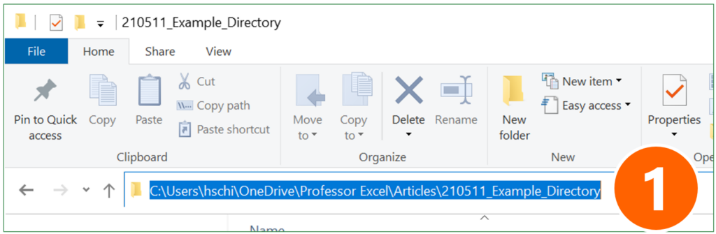
- Copy the folder path from the Windows Explorer like on the screenshot or Mac Finder (for Mac: open file Info (right-click on folder and then on “Get Info”. Select and copy link from “Where” section).
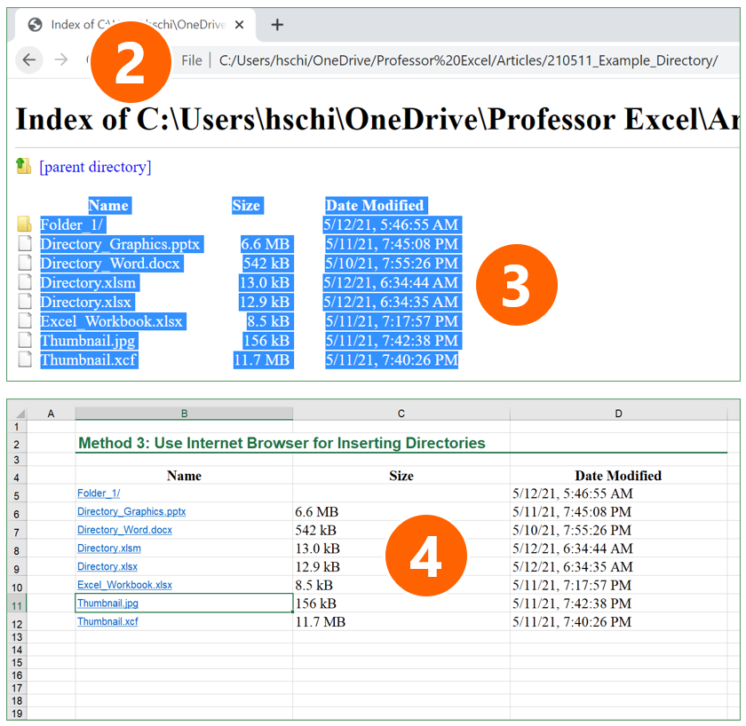
- Open a browser, for example Google Chrome (should be working with most other browsers as well). Paste the previously copied link into the address field.
- Copy the table of files.
- Open Excel and paste the file list.
One comment to this methods: The links (which are also created) usually won’t work in Excel.
Recommendation: Use this if you quickly need a file list (without subfolders), including some file properties such as file size and date last saved.
Method 4: Create a file list with PowerQuery
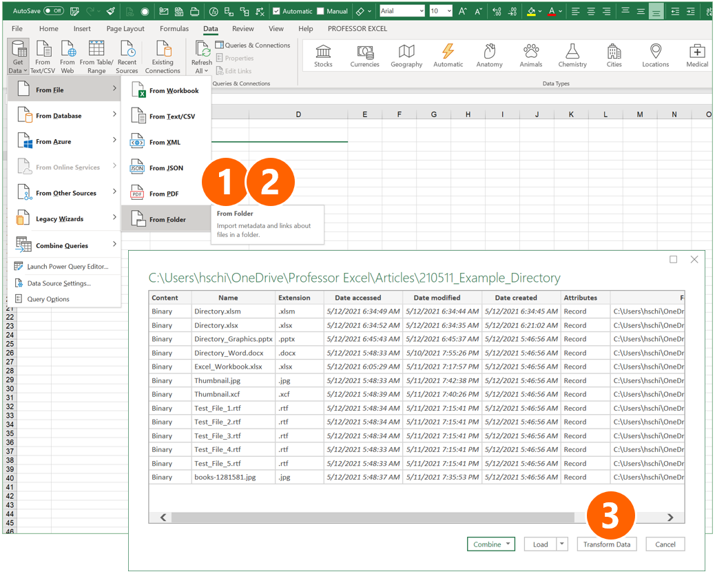
The next method is also among my favorites: It uses PowerQuery and comes with the advantages that it doesn’t require any complex programming or third-party technologies. Also, it can be refreshed easily later on.
- Go to the Data ribbon, click on “Get Data” on the left, and select “From Folder” in the “From File” sub-menu.
- Select the Folder and click on “Open” (not in the screenshot on the right).
- You can now see a preview. Click on “Transform Data”.
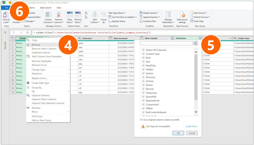
- Remove the first column “Content” (right-click on the heading and click on “Remove”).
- If you want to see more file attributes than shown already in the preview, click on the small arrows of the “Attributes” column and select the attributes.
- Click on Close & Load.
Recommendation: Use this method if you to have lots of file properties. It can later on easily be refreshed.
The Excel add-in Professor Excel Tools offers a function to easily insert directories. It regards subfolders and can insert various file properties:
- Links to files on the drive
- File path
- Date and time last saved
- Date and time created
- File size
- File type
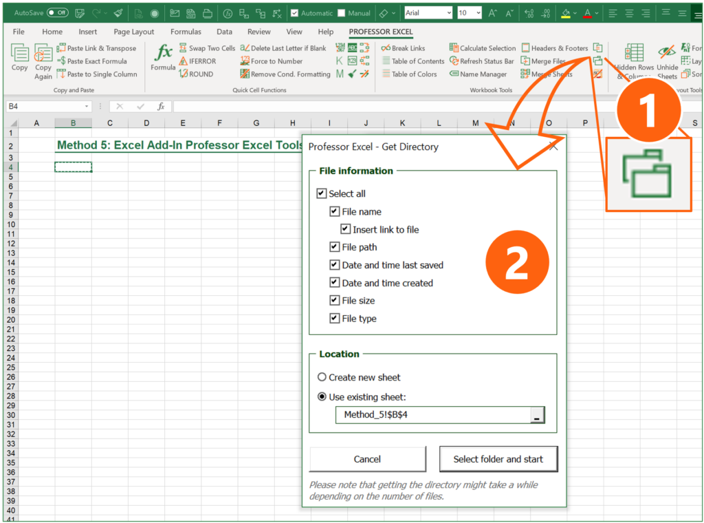
You can further specify, where the directory should be created.
Using the “Get Directory” function is very simple:
- Click on the Directory button on the Professor Excel ribbon.
- Select all the file properties you’d like to show and the location, where the directory table should be placed in your Excel file.
- Click on “Select folder and start”. Then, choose the folder and proceed with ok.
That’s it. Please feel free to download Professor Excel Tools here.
Recommendation: Use this method if you accept third-party add-ins within Excel. If you do, it’s quite convenient and fast.

This function is included in our Excel Add-In ‘Professor Excel Tools’
(No sign-up, download starts directly)
As you can see in the following description, using PowerShell takes quite a lot of steps. It might be useful, though, if you have very large folder structures. Otherwise, try to use a different method.
Open PowerShell and write the directory into a text file
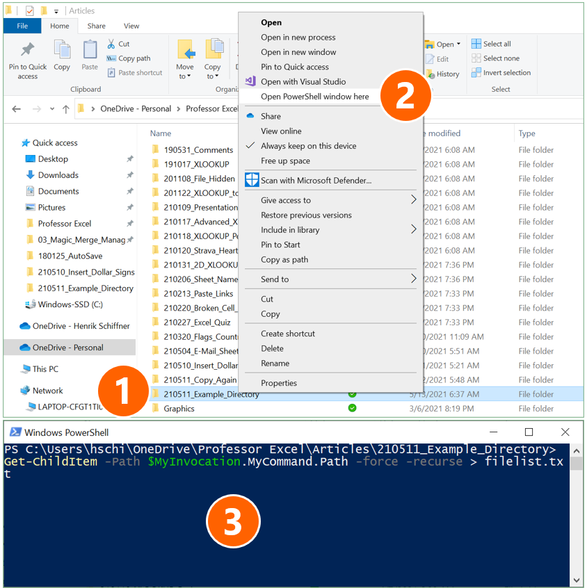
- Navigate to the folder which you want to have the file list from. Hold down the Shift key on the keyboard and right-click on it (if you don’t hold down the Shift key, the option of “Open PowerShell window here” is not available).
- Click on “Open PowerShell window here”.
- Copy and paste the following code and press enter afterwards:
Get-ChildItem -Path $MyInvocation.MyCommand.Path -force -recurse > filelist.txtImport text file into Excel
Open Microsoft Excel.
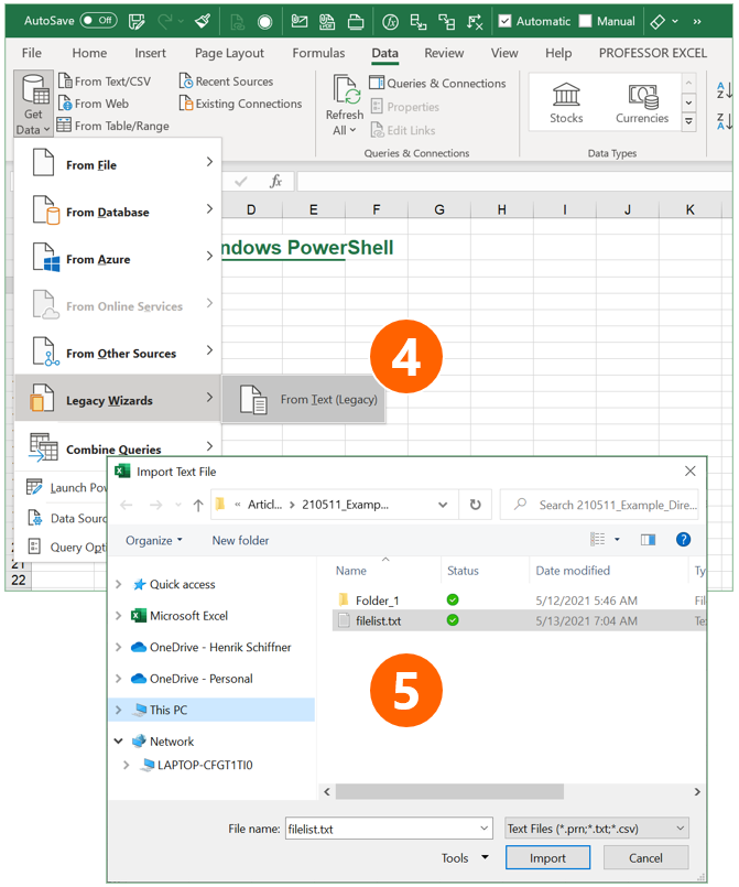
- Open the Text Import Wizard: Go to the Data ribbon, click on “Get Data” on the left, then on “Legacy Wizards” and then on “From Text (Legacy)”. If this option is not available, you can activate it within the Excel settings (check this article for more information).
- Select the file filelist.txt from your folder. In step 3 above it was created within your target folder.
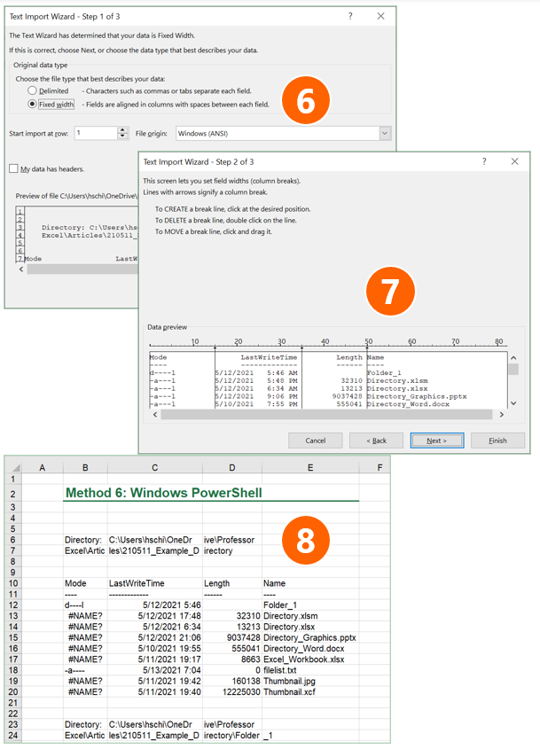
Follow the import steps of the Text Import Wizard on the screen:
- In the first step of three, make sure that “Fixed width” is selected. Click on Next.
- In the lower part of the window, Excel shows a preview of your import. Check here, if the column separators are set correctly: You can move the vertical lines if necessary or add more by clicking on the respective number in the heading of the preview. Then click on Next and in the third step Next again. After that finish the Text Import Wizard by selecting the location where the file list should be placed.
- As you can see in number 8, the file list is inserted, but has some disadvantages: Directory paths are cut, each subfolder has its own block, and so on.
In a nutshell: This method of creating file lists within Microsoft Excel via PowerShell is complex and the results aren’t as good as in the other methods.
Recommendation: Try to avoid this method.
Do you want to boost your productivity in Excel?
Get the Professor Excel ribbon!

Add more than 120 great features to Excel!
Method 7: Let a VBA Macro loop through the files
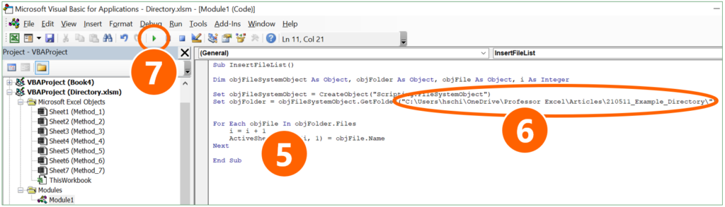
The following VBA code creates a list of all files in a folder. The list will be placed on the currently active worksheet, starting from cell A1. Please make sure that you don’t override anything here.
Sub InsertFileList()

Dim objFileSystemObject As Object, objFolder As Object, objFile As Object, i As Integer

Set objFileSystemObject = CreateObject("Scripting.FileSystemObject")
Set objFolder = objFileSystemObject.GetFolder("Your folder path")

For Each objFile In objFolder.Files
    i = i + 1
    ActiveSheet.Cells(i, 1) = objFile.Name
Next

End Sub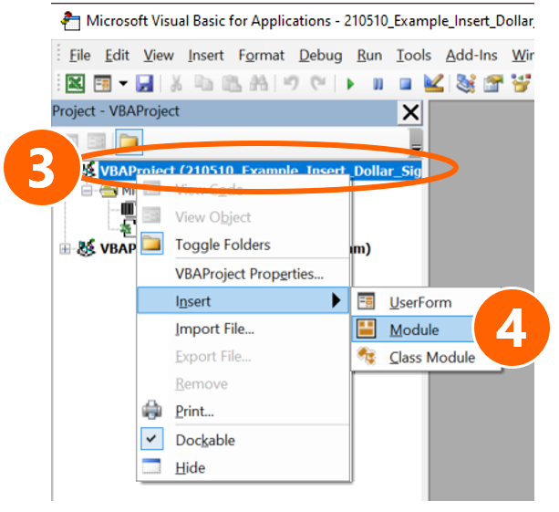
Here is how to use the VBA-Code. If you need more help of how to use VBA macros, please refer to this article.
- Copy the VBA code from above.
- Open the VBA editor by pressing Alt + F11 on the keyboard.
- Insert a new module: Right-click on the active workbook name on the left.
- Go to “Insert” and click on “Module”.
- Paste the code by pressing Ctrl + V on the keyboard.
- Replace Your folder path with the path from your own folder.
- Click on start in the VBA editor.
Download
Please feel free to download all examples from above in this comprehensive Excel workbook. Each method is located on a different worksheet. Just click here and the download starts.
Image by Pexels from Pixabay
Функция INDEX (ИНДЕКС) в Excel используется для получения данных из таблицы, при условии что вы знаете номер строки и столбца, в котором эти данные находятся.
Например, в таблице ниже, вы можете использовать эту функцию для того, чтобы получить результаты экзамена по Физике у Андрея, зная номер строки и столбца, в которых эти данные находятся.

Содержание
- Что возвращает функция
- Синтаксис
- Аргументы функции
- Дополнительная информация
- Примеры использования функции ИНДЕКС в Excel
- Пример 1. Ищем результаты экзамена по физике для Алексея
- Пример 2. Создаем динамический поиск значений с использованием функций ИНДЕКС и ПОИСКПОЗ
- Пример 3. Создаем динамический поиск значений с использованием функций INDEX (ИНДЕКС) и MATCH (ПОИСКПОЗ) и выпадающего списка
- Пример 4. Использование трехстороннего поиска с помощью INDEX (ИНДЕКС) / MATCH (ПОИСКПОЗ)
Что возвращает функция
Возвращает данные из конкретной строки и столбца табличных данных.
Синтаксис
=INDEX (array, row_num, [col_num]) — английская версия
=INDEX (array, row_num, [col_num], [area_num]) — английская версия
=ИНДЕКС(массив; номер_строки; [номер_столбца]) — русская версия
=ИНДЕКС(ссылка; номер_строки; [номер_столбца]; [номер_области]) — русская версия
Аргументы функции
- array (массив) — диапазон ячеек или массив данных для поиска;
- row_num (номер_строки) — номер строки, в которой находятся искомые данные;
- [col_num] ([номер_столбца]) (необязательный аргумент) — номер колонки, в которой находятся искомые данные. Этот аргумент необязательный. Но если в аргументах функции не указаны критерии для row_num (номер_строки), необходимо указать аргумент col_num (номер_столбца);
- [area_num] ([номер_области]) — (необязательный аргумент) — если аргумент массива состоит из нескольких диапазонов, то это число будет использоваться для выбора всех диапазонов.
Дополнительная информация
- Если номер строки или колонки равен “0”, то функция возвращает данные всей строки или колонки;
- Если функция используется перед ссылкой на ячейку (например, A1), она возвращает ссылку на ячейку вместо значения (см. примеры ниже);
- Чаще всего INDEX (ИНДЕКС) используется совместно с функцией MATCH (ПОИСКПОЗ);
- В отличие от функции VLOOKUP (ВПР), функция INDEX (ИНДЕКС) может возвращать данные как справа от искомого значения, так и слева;
- Функция используется в двух формах — Массива данных и Формы ссылки на данные:
— Форма «Массива» используется когда вы хотите найти значения, основанные на конкретных номерах строк и столбцов таблицы;
— Форма «Ссылок на данные» используется при поиске значений в нескольких таблицах (используете аргумент [area_num] ([номер_области]) для выбора таблицы и только потом сориентируете функцию по номеру строки и столбца.
Примеры использования функции ИНДЕКС в Excel
Пример 1. Ищем результаты экзамена по физике для Алексея
Предположим, у вас есть результаты экзаменов в табличном виде по нескольким студентам:
Для того, чтобы найти результаты экзамена по физике для Андрея нам нужна формула:
=INDEX($B$3:$E$9,3,2) — английская версия
=ИНДЕКС($B$3:$E$9;3;2) — русская версия
В формуле мы определили аргумент диапазона данных, где мы будем искать данные $B$3:$E$9. Затем, указали номер строки “3”, в которой находятся результаты экзамена для Андрея, и номер колонки “2”, где находятся результаты экзамена именно по физике.
Пример 2. Создаем динамический поиск значений с использованием функций ИНДЕКС и ПОИСКПОЗ
Не всегда есть возможность указать номера строки и столбца вручную. У вас может быть огромная таблица данных, отображение данных которой вы можете сделать динамическим, чтобы функция автоматически идентифицировала имя или экзамен, указанные в ячейках, и дала правильный результат.
Пример динамического отображения данных ниже:

Для динамического отображения данных мы используем комбинацию функций INDEX (ИНДЕКС) и MATCH (ПОИСКПОЗ).
Вот такая формула поможет нам добиться результата:
=INDEX($B$3:$E$9,MATCH($G$4,$A$3:$A$9,0),MATCH($H$3,$B$2:$E$2,0)) — английская версия
=ИНДЕКС($B$3:$E$9;ПОИСКПОЗ($G$4;$A$3:$A$9;0);ПОИСКПОЗ($H$3;$B$2:$E$2;0)) — русская версия
В формуле выше, не используя сложного программирования, мы с помощью функции MATCH (ПОИСКПОЗ) сделали отображение данных динамическим.
Динамический отображение строки задается следующей частью формулы —
MATCH($G$4,$A$3:$A$9,0) — английская версия
ПОИСКПОЗ($G$4;$A$3:$A$9;0) — русская версия
Она сканирует имена студентов и определяет значение поиска ($G$4 в нашем случае). Затем она возвращает номер строки для поиска в наборе данных. Например, если значение поиска равно Алексей, функция вернет “1”, если это Максим, оно вернет “4” и так далее.
Динамическое отображение данных столбца задается следующей частью формулы —
MATCH($H$3,$B$2:$E$2,0) — английская версия
ПОИСКПОЗ($H$3;$B$2:$E$2;0) — русская версия
Она сканирует имена объектов и определяет значение поиска ($H$3 в нашем случае). Затем она возвращает номер столбца для поиска в наборе данных. Например, если значение поиска Математика, функция вернет “1”, если это Физика, функция вернет “2” и так далее.
Больше лайфхаков в нашем Telegram Подписаться
Пример 3. Создаем динамический поиск значений с использованием функций INDEX (ИНДЕКС) и MATCH (ПОИСКПОЗ) и выпадающего списка
На примере выше мы вручную вводили имена студентов и названия предметов. Вы можете сэкономить время на вводе данных, используя выпадающие списки. Это актуально, когда количество данных огромное.
Используя выпадающие списки, вам нужно просто выбрать из списка имя студента и функция автоматически найдет и подставит необходимые данные.
Пример ниже:

Используя такой подход, вы можете создать удобный дашборд, например для учителя. Ему не придется заниматься фильтрацией данных или прокруткой листа со студентами, для того чтобы найти результаты экзамена конкретного студента, достаточно просто выбрать имя и результаты динамически отразятся в лаконичной и удобной форме.
Для того, чтобы осуществить динамическую подстановку данных с использованием функций INDEX (ИНДЕКС) и MATCH (ПОИСКПОЗ) и выпадающего списка, мы используем ту же формулу, что в Примере 2:
=INDEX($B$3:$E$9,MATCH($G$4,$A$3:$A$9,0),MATCH($H$3,$B$2:$E$2,0)) — английская версия
=ИНДЕКС($B$3:$E$9;ПОИСКПОЗ($G$4;$A$3:$A$9;0);ПОИСКПОЗ($H$3;$B$2:$E$2;0)) — русская версия
Единственное отличие, от Примера 2, мы на месте ввода имени и предмета создадим выпадающие списки:
- Выбираем ячейку, в которой мы хотим отобразить выпадающий список с именами студентов;
- Кликаем на вкладку “Data” => Data Tools => Data Validation;
- В окне Data Validation на вкладке “Settings” в подразделе Allow выбираем “List”;
- В качестве Source нам нужно выбрать диапазон ячеек, в котором указаны имена студентов;
- Кликаем ОК
Теперь у вас есть выпадающий список с именами студентов в ячейке G5. Таким же образом вы можете создать выпадающий список с предметами.
Пример 4. Использование трехстороннего поиска с помощью INDEX (ИНДЕКС) / MATCH (ПОИСКПОЗ)
Функция INDEX (ИНДЕКС) может быть использована для обработки трехсторонних запросов.
Что такое трехсторонний поиск?
В приведенных выше примерах мы использовали одну таблицу с оценками для студентов по разным предметам. Это пример двунаправленного поиска, поскольку мы используем две переменные для получения оценки (имя студента и предмет).
Теперь предположим, что к концу года студент прошел три уровня экзаменов: «Вступительный», «Полугодовой» и «Итоговый экзамен».
Трехсторонний поиск — это возможность получить отметки студента по заданному предмету с указанным уровнем экзамена.
Вот пример трехстороннего поиска:
В приведенном выше примере, кроме выбора имени студента и названия предмета, вы также можете выбрать уровень экзамена. Основываясь на уровне экзамена, формула возвращает соответствующее значение из одной из трех таблиц.
Для таких расчетов нам поможет формула:
=INDEX(($B$3:$E$7,$B$11:$E$15,$B$19:$E$23),MATCH($G$4,$A$3:$A$7,0),MATCH($H$3,$B$2:$E$2,0),IF($H$2=»Вступительный»,1,IF($H$2=»Полугодовой»,2,3))) — английская версия
=ИНДЕКС(($B$3:$E$7;$B$11:$E$15;$B$19:$E$23);ПОИСКПОЗ($G$4;$A$3:$A$7;0);ПОИСКПОЗ($H$3;$B$2:$E$2;0); ЕСЛИ($H$2=»Вступительный»;1;ЕСЛИ($H$2=»Полугодовой»;2;3))) — русская версия
Давайте разберем эту формулу, чтобы понять, как она работает.
Эта формула принимает четыре аргумента. Функция INDEX (ИНДЕКС) — одна из тех функций в Excel, которая имеет более одного синтаксиса.
=INDEX (array, row_num, [col_num]) — английская версия
=INDEX (array, row_num, [col_num], [area_num]) — английская версия
=ИНДЕКС(массив; номер_строки; [номер_столбца]) — русская версия
=ИНДЕКС(ссылка; номер_строки; [номер_столбца]; [номер_области]) — русская версия
По всем вышеприведенным примерам мы использовали первый синтаксис, но для трехстороннего поиска нам нужно использовать второй синтаксис.
Рассмотрим каждую часть формулы на основе второго синтаксиса.
- array (массив) – ($B$3:$E$7,$B$11:$E$15,$B$19:$E$23):Вместо использования одного массива, в данном случае мы использовали три массива в круглых скобках.
- row_num (номер_строки) – MATCH($G$4,$A$3:$A$7,0): функция MATCH (ПОИСКПОЗ) используется для поиска имени студента для ячейки $G$4 из списка всех студентов.
- col_num (номер_столбца) – MATCH($H$3,$B$2:$E$2,0): функция MATCH (ПОИСКПОЗ) используется для поиска названия предмета для ячейки $H$3 из списка всех предметов.
- [area_num] ([номер_области]) – IF($H$2=”Вступительный”,1,IF($H$2=”Полугодовой”,2,3)): Значение номера области сообщает функции INDEX (ИНДЕКС), какой массив с данными выбрать. В этом примере у нас есть три массива в первом аргументе. Если вы выберете «Вступительный» из раскрывающегося меню, функция IF (ЕСЛИ) вернет значение “1”, а функция INDEX (ИНДЕКС) выберут 1-й массив из трех массивов ($B$3:$E$7).
Уверен, что теперь вы подробно изучили работу функции INDEX (ИНДЕКС) в Excel!
Listing the files in a folder is one of the activities which cannot be achieved using normal Excel formulas. I could tell you to turn to VBA macros or PowerQuery, but then any non-VBA and non-PowerQuery users would close this post instantly. But wait! Back away from the close button, there is another option.
For listing files in a folder we can also use a little-known feature from Excel version 4, which still works today, the FILES function.
If you search through the list of Excel functions, FILES is not listed. The FILES function is based on an old Excel feature, which has to be applied in a special way. The instructions below will show you step-by-step how to use it.
Create a named range for the FILES function
The first step is to create a named range, which contains the FILES function. Within the Excel Ribbon click Formulas -> Define Name
Within the New Name window set the following criteria:
- Name: listFiles
Can be any name you wish, but for our example we will be using listFiles. - Refers to: =FILES(Sheet1!$A$1)
Sheet1!$A$1 is the sheet and cell reference containing the name of the folder from which the files are to be listed.
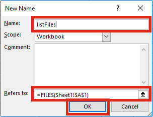
Click OK to close the New Name window.
Apply the function to list files
The second step is to set-up the worksheet to use the named range.
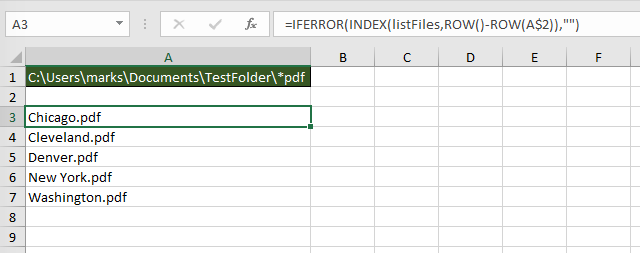
In Cell A1 (or whichever cell reference used in the Refers to box) enter the folder path from which to list the files, followed by an Asterisk ( * ). The Asterisk is the wildcard character to find any text, so it will list all the files in the folder.
Select the cell in which to start the list of files (Cell A3 in the screenshot below), enter the following formula.
=INDEX(listFiles,1)
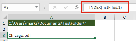
The result of the function will be the name of the first file in the folder.
To retrieve the second file from the folder enter the following formula
=INDEX(listFiles,2)
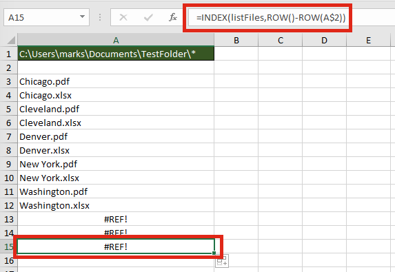
It would be painful to change the file reference number within each formula individually, especially if there are hundreds of files. The good news is, we can use another formula to calculate the reference number automatically.
=INDEX(listFiles,ROW()-ROW(A$2))
The ROW() function is used to retrieve the row number of a cell reference. When used without a cell reference, it returns the row number of the cell in which the function is used. When used with a cell reference it returns the row number of that cell. Using the ROWS function, it is possible to create a sequential list of numbers starting at 1, and increasing by 1 for each cell the formula is copied into.
If the formula is copied down further than the number of files in the folder, it will return a #REF! error.
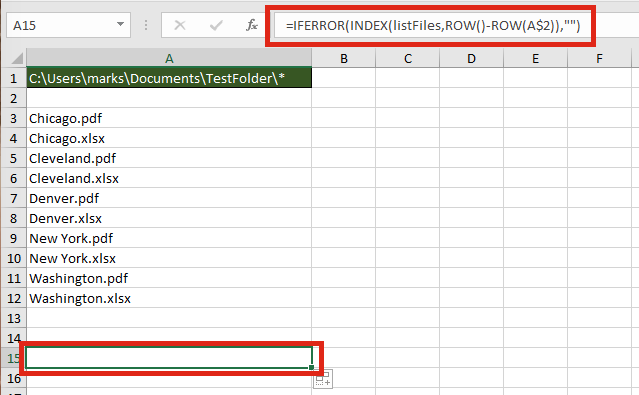
Finally, wrap the formula within an IFERROR function to return a blank cell, rather than an error.
=IFERROR(INDEX(listFiles,ROW()-ROW(A$2)),"")
Listing specific types of files
The FILES function does not just list Excel files; it lists all file types; pdf, csv, mp3, zip, any file type you can think of. By extending the use of wildcards within the file path it is possible to restrict the list to specific file types, or to specific file names.
The screenshot below shows how to return only files with “pdf” as the last three characters of the file name.
The wildcards which can be applied are:
- Question mark ( ? ) – Can take the place of any single character.
- Asterisk ( * ) – Represents any number of characters
- Tilde ( ~ ) – Used as an escape character to search for an asterisk or question mark within the file name, rather than as a wildcard.
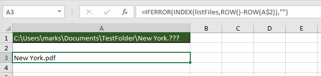
The screenshot below shows how to return only files with the name of “New York.“, followed by exactly three characters.
Advanced uses for the FILES named range
Below are some ideas of how else you could use the FILES function.
Count the number of files
The named range created works like any other named range. However, rather than containing cells, it contains values. Therefore, if you want to calculate the number of files within the folder, or which meet the wildcard pattern use the following formula:
=COUNTA(listFiles)
Create hyperlinks to the files
Wouldn’t it be great to click on the file name to open it automatically? Well . . . just add in the HYPERLINK function and you can.
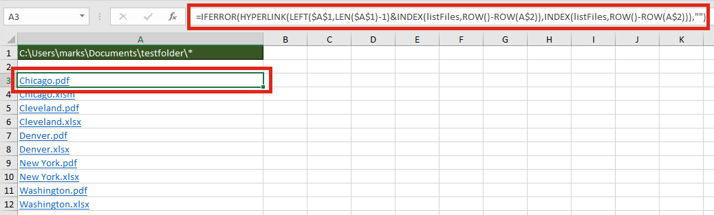
The formula in Cell A3 is:
=IFERROR(HYPERLINK(LEFT($A$1,LEN($A$1)-1)&INDEX(listFiles,ROW()-ROW(A$2)),
INDEX(listFiles,ROW()-ROW(A$2))),"")
Check if a specific file exists within a folder
It isn’t necessary to list all the files to find out if a file exists within the folder. The MATCH function will return the position of the file within the folder.
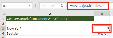
The formula in cell B3 is:
=MATCH(A3,listFiles,0)
In our example, a file which contains the text “New Yor*” exists, as the 7th file, therefore a 7 is returned. Cell B4 displays the #N/A error because “Seattle” does not exist in the folder.
Find the name of the next or previous file
The files returned are in alphabetical order, therefore it is possible to find the next or previous file using the INDEX / MATCH combination.
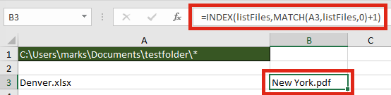
The next file after “Denver.xlsx” is “New York.pdf“. The formula in Cell B3 is:
=INDEX(listFiles,MATCH(A3,listFiles,0)+1)
Retrieve values from each file with INDIRECT
The INDIRECT function can construct a cell reference using text strings. Having retrieved the list of files in a folder, it would be possible to obtain values from those files.
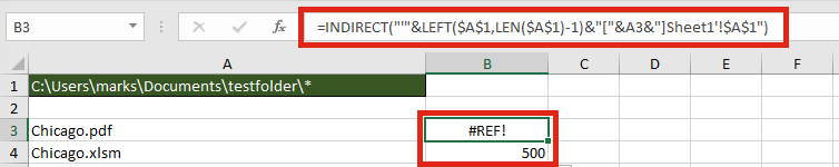
The formula in Cell B3 is:
=INDIRECT("'"&LEFT($A$1,LEN($A$1)-1)&"["&A3&"]Sheet1'!$A$1")
For INDIRECT to calculate correctly the file does need to be open, so this may be a significant flaw in this option.
Usage notes
When working with the FILES function there are a few things to be aware of:
- The file path and file name is not case sensitive
- Files are returned in alphabetical order
- Folders and hidden files are not returned by the function
- The workbook must be saved as a “.xlsm” file format
Further reading
There are variety of other Excel 4 functions available which still work in Excel. Check out this post to find out how to apply them and download the Excel 4 Macro functions reference guide.
If you decide to use a VBA method, check out this post.

About the author
Hey, I’m Mark, and I run Excel Off The Grid.
My parents tell me that at the age of 7 I declared I was going to become a qualified accountant. I was either psychic or had no imagination, as that is exactly what happened. However, it wasn’t until I was 35 that my journey really began.
In 2015, I started a new job, for which I was regularly working after 10pm. As a result, I rarely saw my children during the week. So, I started searching for the secrets to automating Excel. I discovered that by building a small number of simple tools, I could combine them together in different ways to automate nearly all my regular tasks. This meant I could work less hours (and I got pay raises!). Today, I teach these techniques to other professionals in our training program so they too can spend less time at work (and more time with their children and doing the things they love).
Do you need help adapting this post to your needs?
I’m guessing the examples in this post don’t exactly match your situation. We all use Excel differently, so it’s impossible to write a post that will meet everybody’s needs. By taking the time to understand the techniques and principles in this post (and elsewhere on this site), you should be able to adapt it to your needs.
But, if you’re still struggling you should:
- Read other blogs, or watch YouTube videos on the same topic. You will benefit much more by discovering your own solutions.
- Ask the ‘Excel Ninja’ in your office. It’s amazing what things other people know.
- Ask a question in a forum like Mr Excel, or the Microsoft Answers Community. Remember, the people on these forums are generally giving their time for free. So take care to craft your question, make sure it’s clear and concise. List all the things you’ve tried, and provide screenshots, code segments and example workbooks.
- Use Excel Rescue, who are my consultancy partner. They help by providing solutions to smaller Excel problems.
What next?
Don’t go yet, there is plenty more to learn on Excel Off The Grid. Check out the latest posts:
![]()
Download Article
![]()
Download Article
If your Excel workbook contains numerous worksheets, you can add a table of contents that indexes all of your sheets with clickable hyperlinks. This tutorial will teach you how to make an index of sheet names with page numbers in your Excel workbook without complicated VBA scripting, and how to add helpful «back to index» buttons to each sheet to improve navigation.
-

1
Create an index sheet in your workbook. This sheet can be anywhere in your workbook, but you’ll usually want to place the tab at the beginning like a traditional table of contents.
- To create a new sheet, click the + at the bottom of the active worksheet. Then, right-click the new tab, select Rename, and type a name for your sheet like Index or Worksheets.
- You can rearrange sheets by dragging their tabs left or right at the bottom of your workbook.
-
2
Type Page Number into cell A1 of your index sheet. Column A is where you’ll be placing the page numbers for each sheet.
Advertisement
-
3
Type Sheet Name into cell B1 of your index sheet. This will be the column header above your list of worksheets.
-
4
Type Link into cell C1 of your index sheet. This is the column header that will appear above hyperlinks to each worksheet.
-
5
Click the Formulas tab. It’s at the top of Excel.
-
6
Click Define Name. It’s on the «Defined Names» tab at the top of Excel.
-
7
Type SheetList into the «Name» field. This names the formula you’ll be using with the INDEX function.[1]
-
8
Type the formula into the «Refers to» field and click OK. The formula is =REPLACE(GET.WORKBOOK(1),1,FIND("]",GET.WORKBOOK(1)),"").
-
9
Enter page numbers in column A. This is the only part you’ll have to do manually. For example, if your workbook has 20 pages, you’ll type 1 into A2, 2 into A3, etc., and continue numbering down until you’ve entered all 20 page numbers.
- To quickly populate the page numbers, type the first two page numbers into A2 and A3, click A3 to select it, and then drag the square at A3’s bottom-right corner down until you’ve reached the number of pages in your workbook. Then, click the small icon with a + that appears at the bottom-right corner of the column and select Fill Series.
-
10
Type this formula into cell B2 of your index sheet. The formula is =INDEX(SheetList,A2). When you press Enter or Return, you’ll see the name of the first sheet in your workbook.
-
11
Fill the rest of column B with the formula. To do this, just click B2 to select it, and then double-click the square at its bottom-right corner. This adds the name of each worksheet corresponding to the page numbers you typed into column A.
-
12
Type this formula into C2 of your worksheet. The formula is =HYPERLINK("#'"&B2&"'!A1","Go to Sheet"). When you press Enter or Return, you’ll see a hyperlink to the first page in your index called «Go to Sheet.»
-
13
Fill the rest of column C with the formula. To do this, click C2 to select it, and then double-click the square at its bottom-right corner. Now each sheet in your workbook has a clickable hyperlink that takes you right to that page.
-
14
Save your workbook in the macro-enabled format. Because you created a named range, you’ll need to save your workbook in this format.[2]
Here’s how:- Go to File > Save.
- On the pop-up message that warns you about saving a macro-free workbook, click No.
- In the «Save as type» or file format menu, select Excel Macro-Enabled Workbook (*.xlsm) and click Save.


Advertisement
-
1
Click your index or table of contents sheet. If you have a lot of pages in your workbook, it’ll be helpful to readers to add quick «Back to Index» or «Back to Table of Contents» links to each sheet so they don’t have to scroll through lots of worksheet tabs after clicking to that page. Start by opening your index sheet.
-
2
Name the index. To do this, just click the field directly above cell A1, type Index, and then press Enter or Return.
- Don’t worry if the field already contains a cell address.
-
3
Click any of the sheets in your workbook. Now you’ll create your back button. Once you create a back button on one sheet, you can just copy and paste it onto other sheets.
-
4
Click the Insert tab. It’s at the top of the screen.
-
5
Click the Illustrations menu and select Shapes. This option will be in the upper-left area of Excel.
-
6
Click a shape for your button. For example, if you want to create a back-arrow icon sort of like your web browser’s back button, you can click the left-pointing arrow under the «Block Arrows» header.
-
7
Click the location where you want to place the button. Once you click, the shape will appear. If you want, you can change the color and look using the options at the top, and/or resize the shape by dragging any of its corners.
-
8
Type some text onto the shape. The text you type should be something like «Back to Index.» You can double-click the shape to place the cursor and start typing right onto the actual shape
- You might need to drag the corner of the shape to resize it so the text fits.
- To place a text box on or near the shape before typing, just click the Shape Format menu at the top (while the shape is selected), click Text Box in the toolbar, and then click and drag a text box.
- You can stylize the text using the options in Text on the toolbar while the shape is selected.
-
9
Right-click the shape and select Link. This opens the Insert Hyperlink dialog.[3]
-
10
Click the Place in This Document icon. It’s in the left panel.
-
11
Select your index under «Defined Names» and click OK. You might have to click the + next to the column header to see the Index option. This makes the text in the shape a clickable hyperlink that takes you right to the index.
-
12
Copy and paste the hyperlink to other sheets. To do this, just right-click the shape and select Copy. Then, you can paste it onto any other page by right-clicking the desired location and selecting the first icon under «Paste Options» (the one that says «Use Destination Theme» when you hover the mouse over it).


Advertisement
Ask a Question
200 characters left
Include your email address to get a message when this question is answered.
Submit
Advertisement
Thanks for submitting a tip for review!
About This Article
Article SummaryX
To create a table of contents in Excel, you can use the «Defined Name» option to create a formula that indexes all sheet names on a single page. Then, you can use the INDEX function to list the sheet names, as well as the HYPERLINK function to create quick links to each sheet.
Did this summary help you?
Thanks to all authors for creating a page that has been read 55,649 times.
Is this article up to date?
In this guide, we’re going to show you how to create index page of worksheets in Excel with hyperlinks. Using VBA, you can automatically update the hyperlinks after adding or removing sheets.
Download Workbook
First, you need to create a new sheet for the index.
- Create a new sheet.
- Right-click on its tab.
- Select View Code option to open VBA editor for the corresponding sheet.


Alternatively, you can press the Alt + F11 key combination to open the VBA window and select the index sheet from the left pane.
Copy the following code and paste into the editor. Once you pasted the code, it will run every time you open that worksheet.
Code for creating an index of sheets
Private Sub Worksheet_Activate()
    'Define variables
    Dim ws As Worksheet
    Dim row As Long
    row = 1
    'Clear the previous list and add "INDEX" title
    With Me
        .Columns(1).ClearContents
        .Cells(1, 1) = "INDEX"
    End With
    'Loop through each sheet to add a corresponding hyperlink by using the name of the worksheet
    For Each ws In Worksheets
        If ws.Name <> Me.Name And ws.Visible = xlSheetVisible Then
            row = row + 1
            Me.Hyperlinks.Add Anchor:=Me.Cells(row, 1), _
             Address:="", _
             SubAddress:="'" & ws.Name & "'!A1", _
             ScreenTip:="Click to go to sheet " & ws.Name, _
             TextToDisplay:=ws.Name
        End If
    Next ws
    'Adjust the width of first column by the longest worksheet name
    Me.Columns(1).AutoFit
End Sub

You can close the VBA window now and test by opening another sheet other than the index sheet and then go back to the index sheet. The code automatically updates the worksheets that are not hidden.

Remember to save your file as a macro-enabled workbook (xlsm).

Tweaks
The code creates hyperlinks for visible sheets only. We added this check to hide sheets used for calculations or static data which should not be accessible to the end users.
To remove this condition you can remove the And ws.Visible = xlSheetVisible part on the 13th row.
Also, the last line in the subroutine adjusts the width of the first column based on the length of the longest worksheet name. Remove the entire 23rd line, Me.Columns(1).AutoFit, to remove this when creating index of sheets.
The INDEX function returns a value or the reference to a value from within a table or range.

There are two ways to use the INDEX function:
-
If you want to return the value of a specified cell or array of cells, see Array form.
-
If you want to return a reference to specified cells, see Reference form.
Array form
Description
Returns the value of an element in a table or an array, selected by the row and column number indexes.
Use the array form if the first argument to INDEX is an array constant.
Syntax
INDEX(array, row_num, [column_num])
The array form of the INDEX function has the following arguments:
-
array Required. A range of cells or an array constant.
-
If array contains only one row or column, the corresponding row_num or column_num argument is optional.
-
If array has more than one row and more than one column, and only row_num or column_num is used, INDEX returns an array of the entire row or column in array.
-
-
row_num Required, unless column_num is present. Selects the row in array from which to return a value. If row_num is omitted, column_num is required.
-
column_num Optional. Selects the column in array from which to return a value. If column_num is omitted, row_num is required.
Remarks
-
If both the row_num and column_num arguments are used, INDEX returns the value in the cell at the intersection of row_num and column_num.
-
row_num and column_num must point to a cell within array; otherwise, INDEX returns a #REF! error.
-
If you set row_num or column_num to 0 (zero), INDEX returns the array of values for the entire column or row, respectively. To use values returned as an array, enter the INDEX function as an array formula.
Note: If you have a current version of Microsoft 365, then you can input the formula in the top-left-cell of the output range, then press ENTER to confirm the formula as a dynamic array formula. Otherwise, the formula must be entered as a legacy array formula by first selecting the output range, input the formula in the top-left-cell of the output range, then press CTRL+SHIFT+ENTER to confirm it. Excel inserts curly brackets at the beginning and end of the formula for you. For more information on array formulas, see Guidelines and examples of array formulas.
Examples
Example 1
These examples use the INDEX function to find the value in the intersecting cell where a row and a column meet.
Copy the example data in the following table, and paste it in cell A1 of a new Excel worksheet. For formulas to show results, select them, press F2, and then press Enter.
|
Data |
Data |
|
|---|---|---|
|
Apples |
Lemons |
|
|
Bananas |
Pears |
|
|
Formula |
Description |
Result |
|
=INDEX(A2:B3,2,2) |
Value at the intersection of the second row and second column in the range A2:B3. |
Pears |
|
=INDEX(A2:B3,2,1) |
Value at the intersection of the second row and first column in the range A2:B3. |
Bananas |
Example 2
This example uses the INDEX function in an array formula to find the values in two cells specified in a 2×2 array.
Note: If you have a current version of Microsoft 365, then you can input the formula in the top-left-cell of the output range, then press ENTER to confirm the formula as a dynamic array formula. Otherwise, the formula must be entered as a legacy array formula by first selecting two blank cells, input the formula in the top-left-cell of the output range, then press CTRL+SHIFT+ENTER to confirm it. Excel inserts curly brackets at the beginning and end of the formula for you. For more information on array formulas, see Guidelines and examples of array formulas.
|
Formula |
Description |
Result |
|---|---|---|
|
=INDEX({1,2;3,4},0,2) |
Value found in the first row, second column in the array. The array contains 1 and 2 in the first row and 3 and 4 in the second row. |
2 |
|
Value found in the second row, second column in the array (same array as above). |
4 |
|
Top of Page
Reference form
Description
Returns the reference of the cell at the intersection of a particular row and column. If the reference is made up of non-adjacent selections, you can pick the selection to look in.
Syntax
INDEX(reference, row_num, [column_num], [area_num])
The reference form of the INDEX function has the following arguments:
-
reference Required. A reference to one or more cell ranges.
-
If you are entering a non-adjacent range for the reference, enclose reference in parentheses.
-
If each area in reference contains only one row or column, the row_num or column_num argument, respectively, is optional. For example, for a single row reference, use INDEX(reference,,column_num).
-
-
row_num Required. The number of the row in reference from which to return a reference.
-
column_num Optional. The number of the column in reference from which to return a reference.
-
area_num Optional. Selects a range in reference from which to return the intersection of row_num and column_num. The first area selected or entered is numbered 1, the second is 2, and so on. If area_num is omitted, INDEX uses area 1. The areas listed here must all be located on one sheet. If you specify areas that are not on the same sheet as each other, it will cause a #VALUE! error. If you need to use ranges that are located on different sheets from each other, it is recommended that you use the array form of the INDEX function, and use another function to calculate the range that makes up the array. For example, you could use the CHOOSE function to calculate which range will be used.
For example, if Reference describes the cells (A1:B4,D1:E4,G1:H4), area_num 1 is the range A1:B4, area_num 2 is the range D1:E4, and area_num 3 is the range G1:H4.
Remarks
-
After reference and area_num have selected a particular range, row_num and column_num select a particular cell: row_num 1 is the first row in the range, column_num 1 is the first column, and so on. The reference returned by INDEX is the intersection of row_num and column_num.
-
If you set row_num or column_num to 0 (zero), INDEX returns the reference for the entire column or row, respectively.
-
row_num, column_num, and area_num must point to a cell within reference; otherwise, INDEX returns a #REF! error. If row_num and column_num are omitted, INDEX returns the area in reference specified by area_num.
-
The result of the INDEX function is a reference and is interpreted as such by other formulas. Depending on the formula, the return value of INDEX may be used as a reference or as a value. For example, the formula CELL(«width»,INDEX(A1:B2,1,2)) is equivalent to CELL(«width»,B1). The CELL function uses the return value of INDEX as a cell reference. On the other hand, a formula such as 2*INDEX(A1:B2,1,2) translates the return value of INDEX into the number in cell B1.
Examples
Copy the example data in the following table, and paste it in cell A1 of a new Excel worksheet. For formulas to show results, select them, press F2, and then press Enter.
|
Fruit |
Price |
Count |
|---|---|---|
|
Apples |
$0.69 |
40 |
|
Bananas |
$0.34 |
38 |
|
Lemons |
$0.55 |
15 |
|
Oranges |
$0.25 |
25 |
|
Pears |
$0.59 |
40 |
|
Almonds |
$2.80 |
10 |
|
Cashews |
$3.55 |
16 |
|
Peanuts |
$1.25 |
20 |
|
Walnuts |
$1.75 |
12 |
|
Formula |
Description |
Result |
|
=INDEX(A2:C6, 2, 3) |
The intersection of the second row and third column in the range A2:C6, which is the contents of cell C3. |
38 |
|
=INDEX((A1:C6, A8:C11), 2, 2, 2) |
The intersection of the second row and second column in the second area of A8:C11, which is the contents of cell B9. |
1.25 |
|
=SUM(INDEX(A1:C11, 0, 3, 1)) |
The sum of the third column in the first area of the range A1:C11, which is the sum of C1:C11. |
216 |
|
=SUM(B2:INDEX(A2:C6, 5, 2)) |
The sum of the range starting at B2, and ending at the intersection of the fifth row and the second column of the range A2:A6, which is the sum of B2:B6. |
2.42 |
Top of Page
See Also
VLOOKUP function
MATCH function
INDIRECT function
Guidelines and examples of array formulas
Lookup and reference functions (reference)
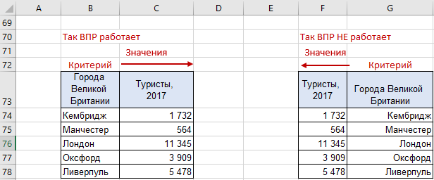
Многие пользователи знают и применяют формулу ВПР. Известно также, что ВПР имеет ряд особенностей и ограничений, которые несложно обойти. Однако есть нюанс, который значительно ограничивает возможности функции ВПР.
ВПР требует, чтобы в диапазоне с искомыми данными столбец критериев всегда был первым слева. Это обстоятельство, конечно, является ограничением ВПР. Как же быть, если искомые данные находятся левее столбца с критерием? Можно, конечно, расположить столбцы в нужном порядке, что в целом, является неплохим выходом из ситуации. Но бывает так, что сделать этого нельзя, или трудно. К примеру, вы работаете в чужом документе или регулярно получаете новый отчет. В общем, нужно решение, не зависящее от расположения столбцов. Такое решение существует.
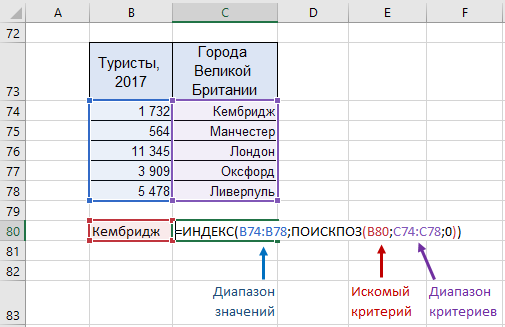
Нужно воспользоваться комбинацией из двух функций: ИНДЕКС и ПОИСКПОЗ. Формула работает следующим образом. ИНДЕКС отсчитывает необходимое количество ячеек вниз в диапазоне искомых значений. Количество отсчитываемых ячеек определяется по столбцу критериев функцией ПОИСКПОЗ. Работу комбинации этих функций удобно рассмотреть с середины, где вначале находится номер ячейки с подходящим критерием, а затем этот номер подставляется в ИНДЕКС.

Таким образом, чтобы подтянуть значение цены, соответствующее первому коду (книге), нужно прописать такую формулу.

Следует обратить внимание на корректность ссылок, чтобы при копировании формулы ничего не «съехало». Протягиваем формулу вниз. Если в таблице, откуда подтягиваются данные, нет искомого критерия, то функция выдает ошибку #Н/Д.

Довольно стандартная ситуация, с которой успешно справляется функция ЕСЛИОШИБКА. Она перехватывает ошибки и вместо них выдает что-либо другое, например, нули.
Конструкция формулы будет следующая:

Вот, собственно, и все.
Таким образом, комбинация функций ИНДЕКС и ПОИСКПОЗ является полной заменой ВПР и обладает дополнительным преимуществом: умеет находить данные слева от столбца с критерием. Кроме того, сами столбцы можно двигать как угодно, лишь бы ссылка не съехала, чего нельзя проделать с ВПР, т.к. количество столбцов там указывается конкретным числом. Посему комбинация ИНДЕКС и ПОИСКПОЗ более универсальна, чем ВПР.
Ниже видеоурок по работе функций ИНДЕКС и ПОИСКПОЗ.
Скачать файл с примером.
Поделиться в социальных сетях:
Функция ИНДЕКС помогает извлекать значение из массива данных. Массив может различаться своей структурой, количеством столбцов и строк и даже количество самих массивов может быть больше одного.
Пример работы функции ИНДЕКС в Excel от простого к сложному
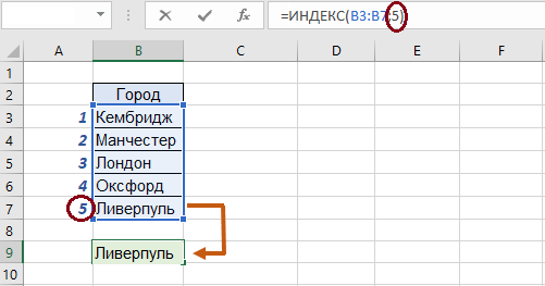
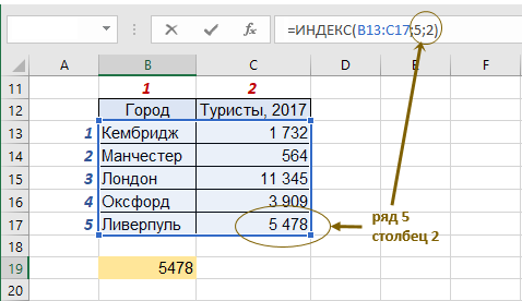
Сначала рассмотрим самый простой пример применения. У нас есть несколько городов. Пусть нашей первой задачей будет извлечь пятый по счету город из нашей одномерной базы данных. Синтаксис нашей формулы будет следующий: ИНДЕКС(массив; номер_строки). Начинаем писать формулу (яч. B9). Первый аргумент – это все города B3:C7, а второй – необходимый нам номер ряда, в котором хранится информация, которую мы хотим получить – пятый город:
Функция возвратила значение с второго ряда нашей таблицы. Теперь дополним нашу таблицу информацией о туристах, посетивших город в 2017 году:
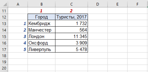
Для дальнейшего ознакомления работы функции расширим задачу до двухмерного массива исходных данных.
Функция ИНДЕКС двумерный и многомерный массив
Теперь наш массив двухмерный. Пусть теперешним заданием будет узнать количество туристов в Ливерпуле. В ячейке B19 пишем формулу. Синтаксис тоже видоизменится: ИНДЕКС(массив; номер_строки; номер_столбца), у нас добавится третий аргумент – номер столбца, в котором хранится нужные нам данные:
Аналогично функция работает с трёхмерными массивами, четырёхмерными и так далее. Теперь давайте рассмотрим, как решать задачи, когда таблиц несколько. Пусть у нас будут города трёх стран с количеством посетителей:
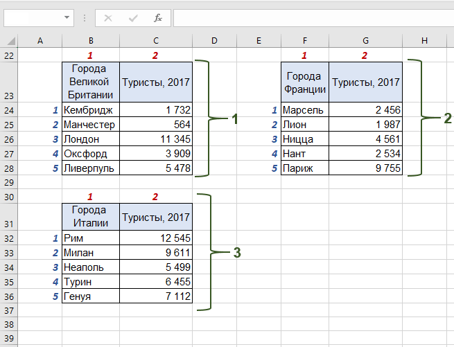
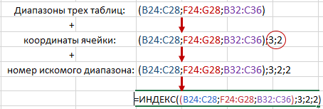
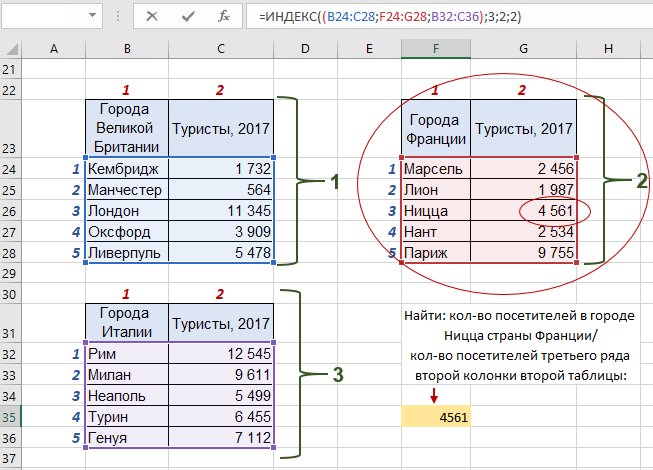
На этот раз у нас три двумерные таблицы – три страны с различными городами и их посетителями. Нам необходимо найти количество туристов в городе Ницца страны Франции или, если перефразировать под наш синтаксис, количество посетителей третьего ряда второй колонки второй таблицы. Первым делом, как и раньше, нам нужно выбрать диапазон. НО теперь их у нас три, а значит, все три мы и выбираем, предварительно взяв в скобки эту часть синтаксиса. После чего добавляем уже знакомые нам координаты искомой информации – строку и столбец, а также номер таблицы, которая содержит искомый нами диапазон:
И получаем готовую формулу с решением поставленной задачи:
Пример формулы комбинации функций ИНДЕКС и СУММ
Функцию ИНДЕКC так же можно комбинировать и с другими функциями. Например, наша база данных содержит дополнительно количество туристов Великобритании за 2018-2019 года, мы хотим узнать сумму туристов:
- за 2018 год.
- по городу Манчестер за весь период.
В этом нам поможет известная любому пользователю несложная функция СУММ. Она охватит результат поиска, сделанным ИНДЕКC и выполнит операцию сложения найденных значений. Чтобы выполнить первую задачу, для начала нам нужно выбрать диапазон с одними числами(без столбца с городами, поскольку будем суммировать численные значения C43:E47). Затем на месте, где мы прописывали номер строки, пишем 0. Благодаря этому ИНДЕКC не будет «искать» данные по строкам, а просто перейдет к следующей операции. А следующая операция – прописываем столбец 2 и получаем ответ на первый пункт:
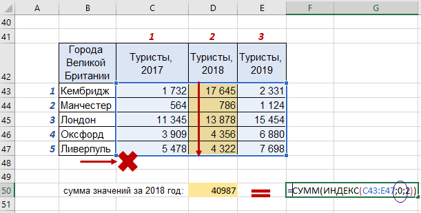
Сумма туристов за 2018 год по пяти городам Великобритании составляет 40 987 людей.
Аналогично этой схеме мы ищем ответ на второй пункт. Только теперь нам нужно считать данные с ряда, поэтому ноль ставим на месте номера столбца:
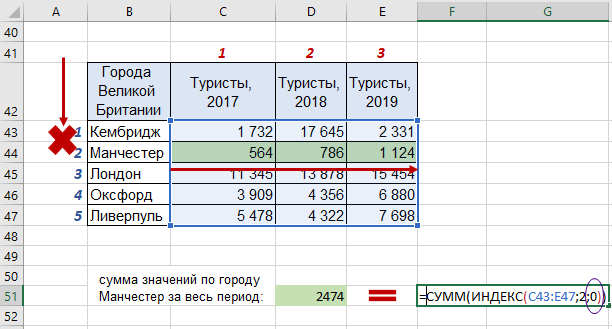
И получаем ответ на второй пункт – всего посетителей за три года в Манчестере было 2 474 человека.
Для примера зачастую используются самые простые задачи и однотипные решения через функцию. Но в работе объем данных всегда больше и сложнее, поэтому для решения таких заданий используют несколько функций или их сочетание. Несколько таких примеров будем рассматривать дальше.
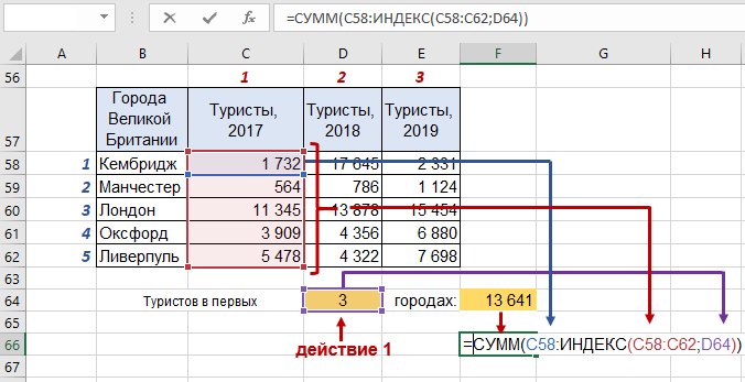
Формулировку функции можно видоизменять в зависимости от постановки задачи. Пусть нам нужно определить и показать сколько туристов вместе было в 2017-м году в первых трёх городах по списку – Кембридже, Манчестере и Лондоне. Тогда мы снова используем функцию СУММ, но в месте, где указывается конец диапазона значений, по которым мы проводим поиск, вставляем нашу ИНДЕКС. Проще говоря, диапазон для суммирования выглядит так: (начало:конец). Началом будет первая ячейка массива, как обычно, а конец мы заменим. Укажем количество городов, по которым будем считать людей (действие 1). Затем, когда будем составлять функцию ИНДЕКC, укажем, что первый аргумент – числовой диапазон всех пяти городов за 2017-й год, а второй – наше кол-во городов (ячейка D64):
Точно так же можно выполнить следующее задание: найти сумму посетителей Оксфорде за 2017-2018 года. В этом случае делаем всё точно так же, только выбираем горизонтальный диапазон C61:E61 :
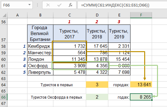
В конце необязательно ссылаться на ячейку с написанным количеством искомых значений, можно сразу писать цифру 3 в первом примере и цифру 2 во втором примере, всё будет работать точно так же:
и
идентичны.
Комбинирование нескольких функций могут делать то же, что и одна отдельная функция, но при этом быть менее требовательными к расположению данных, к их размерам или количеству.
Формула ИНДЕКС и ПОИСКПОЗ лучшая замена функции ВПР
Существуют весьма весомые аргументы преимущества использования формулы ИНДЕКС и ПОИСКПОЗ в Excel лучше, чем функция ВПР. Если вы уже знакомы с функцией ВПР, то наверняка знаете, что для её корректной работы искомые данные всегда должны располагаться по правую сторону от критериев:
Получается, что для работы сначала нужно упорядочить столбцы в соответствии с требованиями, а только потом совершать действия. Но иногда сама структура отчета или сводки, с которой нам нужно иметь дело, не позволяет совершать перестановки. Тогда нам очень кстати пригодится ИНДЕКС в сочетании с функцией ПОИСКПОЗ. Синтаксис ИНДЕКСА: (массив; номер_строки; номер_столбца). На первой позиции у нас будет диапазон значений (туристы, 2017), вместо следующих двух пишем ПОИСКПОЗ (искомый критерий;диапазон критериев; 0 (для точного результата)):
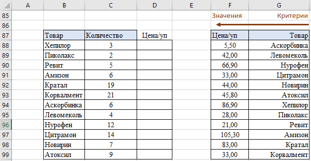
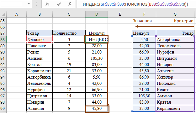
Рассмотрим более наглядный и реальный пример, где можно заменить ВПР. У нас есть два отчета: один — о количестве продаж определенного товара, а второй – о цене на упаковку одного товара. И как раз вторая таблица имеет такое расположение столбцов, которое не позволяет использовать нам ВПР – первыми занимают место значения, а вторыми – критерии:
Для того чтобы выполнить заполнение первой таблицы, делаем точно также, как в предыдущем примере – в ячейке D88 пишем ИНДЕКС, первым делом указываем столбец, где находятся искомые значения (цена за упаковку). Затем нужно указать, где нам искать соответствующие критерию значения — подстраиваем ПОИСКПОЗ под наше решение: выбираем искомый критерий (Хепилор), затем массив искомых критериев со второй таблицы:
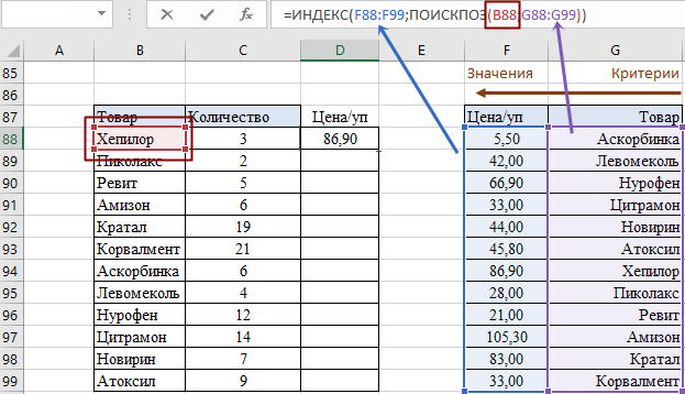
Теперь просто копируем формулу до конца столбца, но не забываем закрепить ссылки, иначе массив будет спускаться дальше и мы получим некорректные значения. Наша таблица готова:
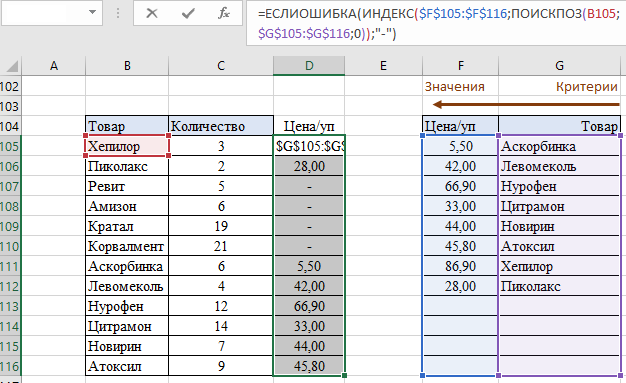
Если у нас нет данных во второй таблице о цене и препаратах, у нас будет в ячейке ошибка #Н/Д. Теперь к нашим ранее использованным функциям добавим ЕСЛИОШИБКА, которая нам поможет изменить внешний вид отчета, сделать его более понятным для читателя. Опять же, поскольку у нас вторая таблица не соответствует требованиям ВПР, на помощь приходит ИНДЕКС+ПОИСКПОЗ. Усложняем уже имеющуюся формулу, добавляя ЕСЛИОШИБКА, указывая, что при отсутствии данных, мы хотим видеть прочерк:
 Скачать примеры функции ИНДЕКС и ПОИСКПОЗ в Excel
Таким образом формула из комбинации функций ИНДЕКС и ПОИСПОЗ работают лучше популярной функции ВПР и не имеют никаких ограничений для выборки данных из таблицы даже по нескольким условиям.