
The INDEX function returns a value or the reference to a value from within a table or range.

There are two ways to use the INDEX function:
-
If you want to return the value of a specified cell or array of cells, see Array form.
-
If you want to return a reference to specified cells, see Reference form.
Array form
Description
Returns the value of an element in a table or an array, selected by the row and column number indexes.
Use the array form if the first argument to INDEX is an array constant.
Syntax
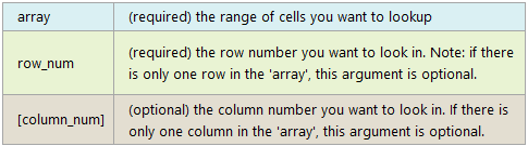
INDEX(array, row_num, [column_num])
The array form of the INDEX function has the following arguments:
-
array Required. A range of cells or an array constant.
-
If array contains only one row or column, the corresponding row_num or column_num argument is optional.
-
If array has more than one row and more than one column, and only row_num or column_num is used, INDEX returns an array of the entire row or column in array.
-
-
row_num Required, unless column_num is present. Selects the row in array from which to return a value. If row_num is omitted, column_num is required.
-
column_num Optional. Selects the column in array from which to return a value. If column_num is omitted, row_num is required.
Remarks
-
If both the row_num and column_num arguments are used, INDEX returns the value in the cell at the intersection of row_num and column_num.
-
row_num and column_num must point to a cell within array; otherwise, INDEX returns a #REF! error.
-
If you set row_num or column_num to 0 (zero), INDEX returns the array of values for the entire column or row, respectively. To use values returned as an array, enter the INDEX function as an array formula.
Note: If you have a current version of Microsoft 365, then you can input the formula in the top-left-cell of the output range, then press ENTER to confirm the formula as a dynamic array formula. Otherwise, the formula must be entered as a legacy array formula by first selecting the output range, input the formula in the top-left-cell of the output range, then press CTRL+SHIFT+ENTER to confirm it. Excel inserts curly brackets at the beginning and end of the formula for you. For more information on array formulas, see Guidelines and examples of array formulas.
Examples
Example 1
These examples use the INDEX function to find the value in the intersecting cell where a row and a column meet.
Copy the example data in the following table, and paste it in cell A1 of a new Excel worksheet. For formulas to show results, select them, press F2, and then press Enter.
|
Data |
Data |
|
|---|---|---|
|
Apples |
Lemons |
|
|
Bananas |
Pears |
|
|
Formula |
Description |
Result |
|
=INDEX(A2:B3,2,2) |
Value at the intersection of the second row and second column in the range A2:B3. |
Pears |
|
=INDEX(A2:B3,2,1) |
Value at the intersection of the second row and first column in the range A2:B3. |
Bananas |
Example 2
This example uses the INDEX function in an array formula to find the values in two cells specified in a 2×2 array.
Note: If you have a current version of Microsoft 365, then you can input the formula in the top-left-cell of the output range, then press ENTER to confirm the formula as a dynamic array formula. Otherwise, the formula must be entered as a legacy array formula by first selecting two blank cells, input the formula in the top-left-cell of the output range, then press CTRL+SHIFT+ENTER to confirm it. Excel inserts curly brackets at the beginning and end of the formula for you. For more information on array formulas, see Guidelines and examples of array formulas.
|
Formula |
Description |
Result |
|---|---|---|
|
=INDEX({1,2;3,4},0,2) |
Value found in the first row, second column in the array. The array contains 1 and 2 in the first row and 3 and 4 in the second row. |
2 |
|
Value found in the second row, second column in the array (same array as above). |
4 |
|
Top of Page
Reference form
Description
Returns the reference of the cell at the intersection of a particular row and column. If the reference is made up of non-adjacent selections, you can pick the selection to look in.
Syntax
INDEX(reference, row_num, [column_num], [area_num])
The reference form of the INDEX function has the following arguments:
-
reference Required. A reference to one or more cell ranges.
-
If you are entering a non-adjacent range for the reference, enclose reference in parentheses.
-
If each area in reference contains only one row or column, the row_num or column_num argument, respectively, is optional. For example, for a single row reference, use INDEX(reference,,column_num).
-
-
row_num Required. The number of the row in reference from which to return a reference.
-
column_num Optional. The number of the column in reference from which to return a reference.
-
area_num Optional. Selects a range in reference from which to return the intersection of row_num and column_num. The first area selected or entered is numbered 1, the second is 2, and so on. If area_num is omitted, INDEX uses area 1. The areas listed here must all be located on one sheet. If you specify areas that are not on the same sheet as each other, it will cause a #VALUE! error. If you need to use ranges that are located on different sheets from each other, it is recommended that you use the array form of the INDEX function, and use another function to calculate the range that makes up the array. For example, you could use the CHOOSE function to calculate which range will be used.
For example, if Reference describes the cells (A1:B4,D1:E4,G1:H4), area_num 1 is the range A1:B4, area_num 2 is the range D1:E4, and area_num 3 is the range G1:H4.
Remarks
-
After reference and area_num have selected a particular range, row_num and column_num select a particular cell: row_num 1 is the first row in the range, column_num 1 is the first column, and so on. The reference returned by INDEX is the intersection of row_num and column_num.
-
If you set row_num or column_num to 0 (zero), INDEX returns the reference for the entire column or row, respectively.
-
row_num, column_num, and area_num must point to a cell within reference; otherwise, INDEX returns a #REF! error. If row_num and column_num are omitted, INDEX returns the area in reference specified by area_num.
-
The result of the INDEX function is a reference and is interpreted as such by other formulas. Depending on the formula, the return value of INDEX may be used as a reference or as a value. For example, the formula CELL(«width»,INDEX(A1:B2,1,2)) is equivalent to CELL(«width»,B1). The CELL function uses the return value of INDEX as a cell reference. On the other hand, a formula such as 2*INDEX(A1:B2,1,2) translates the return value of INDEX into the number in cell B1.
Examples
Copy the example data in the following table, and paste it in cell A1 of a new Excel worksheet. For formulas to show results, select them, press F2, and then press Enter.
|
Fruit |
Price |
Count |
|---|---|---|
|
Apples |
$0.69 |
40 |
|
Bananas |
$0.34 |
38 |
|
Lemons |
$0.55 |
15 |
|
Oranges |
$0.25 |
25 |
|
Pears |
$0.59 |
40 |
|
Almonds |
$2.80 |
10 |
|
Cashews |
$3.55 |
16 |
|
Peanuts |
$1.25 |
20 |
|
Walnuts |
$1.75 |
12 |
|
Formula |
Description |
Result |
|
=INDEX(A2:C6, 2, 3) |
The intersection of the second row and third column in the range A2:C6, which is the contents of cell C3. |
38 |
|
=INDEX((A1:C6, A8:C11), 2, 2, 2) |
The intersection of the second row and second column in the second area of A8:C11, which is the contents of cell B9. |
1.25 |
|
=SUM(INDEX(A1:C11, 0, 3, 1)) |
The sum of the third column in the first area of the range A1:C11, which is the sum of C1:C11. |
216 |
|
=SUM(B2:INDEX(A2:C6, 5, 2)) |
The sum of the range starting at B2, and ending at the intersection of the fifth row and the second column of the range A2:A6, which is the sum of B2:B6. |
2.42 |
Top of Page
See Also
VLOOKUP function
MATCH function
INDIRECT function
Guidelines and examples of array formulas
Lookup and reference functions (reference)
Содержание
- INDEX function
- Array form
- Description
- Syntax
- Remarks
- Examples
- Example 1
- Example 2
- Reference form
- Description
- Syntax
- Remarks
- Examples
- Look up values with VLOOKUP, INDEX, or MATCH
- Using INDEX and MATCH instead of VLOOKUP
- Give it a try
- VLOOKUP Example at work
- INDEX Function
- Related functions
- Summary
- Purpose
- Return value
- Arguments
- Syntax
- Usage notes
- Basic usage
- INDEX and MATCH
- INDEX and MATCH with horizontal table
- Entire row / column
- Reference as result
- Two forms
- Array form
- Reference form
INDEX function
The INDEX function returns a value or the reference to a value from within a table or range.
There are two ways to use the INDEX function:
If you want to return the value of a specified cell or array of cells, see Array form.
If you want to return a reference to specified cells, see Reference form.
Array form
Description
Returns the value of an element in a table or an array, selected by the row and column number indexes.
Use the array form if the first argument to INDEX is an array constant.
Syntax
INDEX(array, row_num, [column_num])
The array form of the INDEX function has the following arguments:
array Required. A range of cells or an array constant.
If array contains only one row or column, the corresponding row_num or column_num argument is optional.
If array has more than one row and more than one column, and only row_num or column_num is used, INDEX returns an array of the entire row or column in array.
row_num Required, unless column_num is present. Selects the row in array from which to return a value. If row_num is omitted, column_num is required.
column_num Optional. Selects the column in array from which to return a value. If column_num is omitted, row_num is required.
If both the row_num and column_num arguments are used, INDEX returns the value in the cell at the intersection of row_num and column_num.
row_num and column_num must point to a cell within array; otherwise, INDEX returns a #REF! error.
If you set row_num or column_num to 0 (zero), INDEX returns the array of values for the entire column or row, respectively. To use values returned as an array, enter the INDEX function as an array formula.
Note: If you have a current version of Microsoft 365, then you can input the formula in the top-left-cell of the output range, then press ENTER to confirm the formula as a dynamic array formula. Otherwise, the formula must be entered as a legacy array formula by first selecting the output range, input the formula in the top-left-cell of the output range, then press CTRL+SHIFT+ENTER to confirm it. Excel inserts curly brackets at the beginning and end of the formula for you. For more information on array formulas, see Guidelines and examples of array formulas.
Examples
Example 1
These examples use the INDEX function to find the value in the intersecting cell where a row and a column meet.
Copy the example data in the following table, and paste it in cell A1 of a new Excel worksheet. For formulas to show results, select them, press F2, and then press Enter.
Value at the intersection of the second row and second column in the range A2:B3.
Value at the intersection of the second row and first column in the range A2:B3.
Example 2
This example uses the INDEX function in an array formula to find the values in two cells specified in a 2×2 array.
Note: If you have a current version of Microsoft 365, then you can input the formula in the top-left-cell of the output range, then press ENTER to confirm the formula as a dynamic array formula. Otherwise, the formula must be entered as a legacy array formula by first selecting two blank cells, input the formula in the top-left-cell of the output range, then press CTRL+SHIFT+ENTER to confirm it. Excel inserts curly brackets at the beginning and end of the formula for you. For more information on array formulas, see Guidelines and examples of array formulas.
Value found in the first row, second column in the array. The array contains 1 and 2 in the first row and 3 and 4 in the second row.
Value found in the second row, second column in the array (same array as above).
Reference form
Description
Returns the reference of the cell at the intersection of a particular row and column. If the reference is made up of non-adjacent selections, you can pick the selection to look in.
Syntax
INDEX(reference, row_num, [column_num], [area_num])
The reference form of the INDEX function has the following arguments:
reference Required. A reference to one or more cell ranges.
If you are entering a non-adjacent range for the reference, enclose reference in parentheses.
If each area in reference contains only one row or column, the row_num or column_num argument, respectively, is optional. For example, for a single row reference, use INDEX(reference,,column_num).
row_num Required. The number of the row in reference from which to return a reference.
column_num Optional. The number of the column in reference from which to return a reference.
area_num Optional. Selects a range in reference from which to return the intersection of row_num and column_num. The first area selected or entered is numbered 1, the second is 2, and so on. If area_num is omitted, INDEX uses area 1. The areas listed here must all be located on one sheet. If you specify areas that are not on the same sheet as each other, it will cause a #VALUE! error. If you need to use ranges that are located on different sheets from each other, it is recommended that you use the array form of the INDEX function, and use another function to calculate the range that makes up the array. For example, you could use the CHOOSE function to calculate which range will be used.
For example, if Reference describes the cells (A1:B4,D1:E4,G1:H4), area_num 1 is the range A1:B4, area_num 2 is the range D1:E4, and area_num 3 is the range G1:H4.
After reference and area_num have selected a particular range, row_num and column_num select a particular cell: row_num 1 is the first row in the range, column_num 1 is the first column, and so on. The reference returned by INDEX is the intersection of row_num and column_num.
If you set row_num or column_num to 0 (zero), INDEX returns the reference for the entire column or row, respectively.
row_num, column_num, and area_num must point to a cell within reference; otherwise, INDEX returns a #REF! error. If row_num and column_num are omitted, INDEX returns the area in reference specified by area_num.
The result of the INDEX function is a reference and is interpreted as such by other formulas. Depending on the formula, the return value of INDEX may be used as a reference or as a value. For example, the formula CELL(«width»,INDEX(A1:B2,1,2)) is equivalent to CELL(«width»,B1). The CELL function uses the return value of INDEX as a cell reference. On the other hand, a formula such as 2*INDEX(A1:B2,1,2) translates the return value of INDEX into the number in cell B1.
Examples
Copy the example data in the following table, and paste it in cell A1 of a new Excel worksheet. For formulas to show results, select them, press F2, and then press Enter.
Источник
Look up values with VLOOKUP, INDEX, or MATCH
Tip: Try using the new XLOOKUP and XMATCH functions, improved versions of the functions described in this article. These new functions work in any direction and return exact matches by default, making them easier and more convenient to use than their predecessors.
Suppose that you have a list of office location numbers, and you need to know which employees are in each office. The spreadsheet is huge, so you might think it is challenging task. It’s actually quite easy to do with a lookup function.
The VLOOKUP and HLOOKUP functions, together with INDEX and MATCH, are some of the most useful functions in Excel.
Note: The Lookup Wizard feature is no longer available in Excel.
Here’s an example of how to use VLOOKUP.
In this example, B2 is the first argument—an element of data that the function needs to work. For VLOOKUP, this first argument is the value that you want to find. This argument can be a cell reference, or a fixed value such as «smith» or 21,000. The second argument is the range of cells, C2-:E7, in which to search for the value you want to find. The third argument is the column in that range of cells that contains the value that you seek.
The fourth argument is optional. Enter either TRUE or FALSE. If you enter TRUE, or leave the argument blank, the function returns an approximate match of the value you specify in the first argument. If you enter FALSE, the function will match the value provide by the first argument. In other words, leaving the fourth argument blank—or entering TRUE—gives you more flexibility.
This example shows you how the function works. When you enter a value in cell B2 (the first argument), VLOOKUP searches the cells in the range C2:E7 (2nd argument) and returns the closest approximate match from the third column in the range, column E (3rd argument).
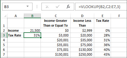
The fourth argument is empty, so the function returns an approximate match. If it didn’t, you’d have to enter one of the values in columns C or D to get a result at all.
When you’re comfortable with VLOOKUP, the HLOOKUP function is equally easy to use. You enter the same arguments, but it searches in rows instead of columns.
Using INDEX and MATCH instead of VLOOKUP
There are certain limitations with using VLOOKUP—the VLOOKUP function can only look up a value from left to right. This means that the column containing the value you look up should always be located to the left of the column containing the return value. Now if your spreadsheet isn’t built this way, then do not use VLOOKUP. Use the combination of INDEX and MATCH functions instead.
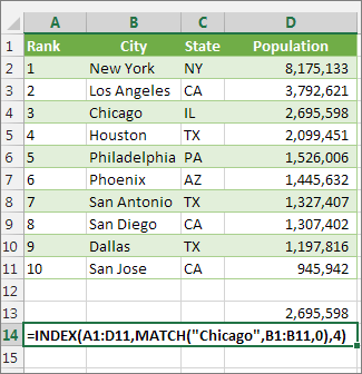
This example shows a small list where the value we want to search on, Chicago, isn’t in the leftmost column. So, we can’t use VLOOKUP. Instead, we’ll use the MATCH function to find Chicago in the range B1:B11. It’s found in row 4. Then, INDEX uses that value as the lookup argument, and finds the population for Chicago in the 4th column (column D). The formula used is shown in cell A14.
For more examples of using INDEX and MATCH instead of VLOOKUP, see the article https://www.mrexcel.com/excel-tips/excel-vlookup-index-match/ by Bill Jelen, Microsoft MVP.
Give it a try
If you want to experiment with lookup functions before you try them out with your own data, here’s some sample data.
VLOOKUP Example at work
Copy the following data into a blank spreadsheet.
Tip: Before you paste the data into Excel, set the column widths for columns A through C to 250 pixels, and click Wrap Text ( Home tab, Alignment group).
Источник
INDEX Function

Summary
The Excel INDEX function returns the value at a given location in a range or array. You can use INDEX to retrieve individual values, or entire rows and columns. The MATCH function is often used together with INDEX to provide row and column numbers.
Purpose
Return value
Arguments
- array — A range of cells, or an array constant.
- row_num — The row position in the reference or array.
- col_num — [optional] The column position in the reference or array.
- area_num — [optional] The range in reference that should be used.
Syntax
Usage notes
The INDEX function returns the value at a given location in a range or array. INDEX is a powerful and versatile function. You can use INDEX to retrieve individual values, or entire rows and columns. INDEX is frequently used together with the MATCH function. In this scenario, the MATCH function locates and feeds a position to the INDEX function, and INDEX returns the value at that position.
In the most common usage, INDEX takes three arguments: array, row_num, and col_num. Array is the range or array from which to retrieve values. Row_num is the row number from which to retrieve a value, and col_num is the column number at which to retrieve a value. Col_num is optional and not needed when array is one-dimensional.
In the example shown above, the goal is to get the diameter of the planet Jupiter. Because Jupiter is the fifth planet in the list, and Diameter is the third column, the formula in G7 is:
The formula above is of limited value because the row number and column number have been hard-coded. Typically, the MATCH function would be used inside INDEX to provide these numbers. For a detailed explanation with many examples, see: How to use INDEX and MATCH.
Basic usage
INDEX gets a value at a given location in a range of cells based on numeric position. When the range is one-dimensional, you only need to supply a row number. When the range is two-dimensional, you’ll need to supply both the row and column number. For example, to get the third item from the one-dimensional range A1:A5:
The formulas below show how INDEX can be used to get a value from a two-dimensional range:
INDEX and MATCH
In the examples above, the position is «hardcoded». Typically, the MATCH function is used to find positions for INDEX. For example, in the screen below, the MATCH function is used to locate «Mars» (G6) in row 3 and feed that position to INDEX. The formula in G7 is:

MATCH provides the row number (4) to INDEX. The column number is still hardcoded as 3.
INDEX and MATCH with horizontal table
In the screen below, the table above has been transposed horizontally. The MATCH function returns the column number (4) and the row number is hardcoded as 2. The formula in C10 is:

For a detailed explanation with many examples, see: How to use INDEX and MATCH
Entire row / column
INDEX can be used to return entire columns or rows like this:
where n represents the number of the column or row to return. This example shows a practical application of this idea.
Reference as result
It’s important to note that the INDEX function returns a reference as a result. For example, in the following formula, INDEX returns A2:
In a typical formula, you’ll see the value in cell A2 as the result, so it’s not obvious that INDEX is returning a reference. However, this is a useful feature in formulas like this one, which uses INDEX to create a dynamic named range. You can use the CELL function to report the reference returned by INDEX.
Two forms
The INDEX function has two forms: array and reference. Both forms have the same behavior – INDEX returns a reference in an array based on a given row and column location. The difference is that the reference form of INDEX allows more than one array, along with an optional argument to select which array should be used. Most formulas use the array form of INDEX, but both forms are discussed below.
Array form
In the array form of INDEX, the first parameter is an array, which is supplied as a range of cells or an array constant. The syntax for the array form of INDEX is:
- If both row_num and col_num are supplied, INDEX returns the value in the cell at the intersection of row_num and col_num.
- If row_num is set to zero, INDEX returns an array of values for an entire column. To use these array values, you can enter the INDEX function as an array formula in horizontal range, or feed the array into another function.
- If col_num is set to zero, INDEX returns an array of values for an entire row. To use these array values, you can enter the INDEX function as an array formula in vertical range, or feed the array into another function.
Reference form
In the reference form of INDEX, the first parameter is a reference to one or more ranges, and a fourth optional argument, area_num, is provided to select the appropriate range. The syntax for the reference form of INDEX is:
Just like the array form of INDEX, the reference form of INDEX returns the reference of the cell at the intersection row_num and col_num. The difference is that the reference argument contains more than one range, and area_num selects which range should be used. The area_num is argument is supplied as a number that acts like a numeric index. The first array inside reference is 1, the second array is 2, and so on.
For example, in the formula below, area_num is supplied as 2, which refers to the range A7:C10:
In the above formula, INDEX will return the value at row 1 and column 3 of A7:C10.
- Multiple ranges in reference are separated by commas and enclosed in parentheses.
- All ranges must on one sheet or INDEX will return a #VALUE error. Use the CHOOSE function as a workaround.
Источник
The INDEX function returns the value at a given location in a range or array. INDEX is a powerful and versatile function. You can use INDEX to retrieve individual values, or entire rows and columns. INDEX is frequently used together with the MATCH function. In this scenario, the MATCH function locates and feeds a position to the INDEX function, and INDEX returns the value at that position.
In the most common usage, INDEX takes three arguments: array, row_num, and col_num. Array is the range or array from which to retrieve values. Row_num is the row number from which to retrieve a value, and col_num is the column number at which to retrieve a value. Col_num is optional and not needed when array is one-dimensional.
In the example shown above, the goal is to get the diameter of the planet Jupiter. Because Jupiter is the fifth planet in the list, and Diameter is the third column, the formula in G7 is:
=INDEX(B5:E13,5,3) // diameter of Jupiter
The formula above is of limited value because the row number and column number have been hard-coded. Typically, the MATCH function would be used inside INDEX to provide these numbers. For a detailed explanation with many examples, see: How to use INDEX and MATCH.
Basic usage
INDEX gets a value at a given location in a range of cells based on numeric position. When the range is one-dimensional, you only need to supply a row number. When the range is two-dimensional, you’ll need to supply both the row and column number. For example, to get the third item from the one-dimensional range A1:A5:
=INDEX(A1:A5,3) // returns value in A3
The formulas below show how INDEX can be used to get a value from a two-dimensional range:
=INDEX(A1:B5,2,2) // returns value in B2
=INDEX(A1:B5,3,1) // returns value in A3
INDEX and MATCH
In the examples above, the position is «hardcoded». Typically, the MATCH function is used to find positions for INDEX. For example, in the screen below, the MATCH function is used to locate «Mars» (G6) in row 3 and feed that position to INDEX. The formula in G7 is:
=INDEX(B5:E13,MATCH(G6,B5:B13,0),3)
MATCH provides the row number (4) to INDEX. The column number is still hardcoded as 3.
INDEX and MATCH with horizontal table
In the screen below, the table above has been transposed horizontally. The MATCH function returns the column number (4) and the row number is hardcoded as 2. The formula in C10 is:
=INDEX(C4:K6,2,MATCH(C9,C4:K4,0))
For a detailed explanation with many examples, see: How to use INDEX and MATCH
Entire row / column
INDEX can be used to return entire columns or rows like this:
=INDEX(range,0,n) // entire column
=INDEX(range,n,0) // entire row
where n represents the number of the column or row to return. This example shows a practical application of this idea.
Reference as result
It’s important to note that the INDEX function returns a reference as a result. For example, in the following formula, INDEX returns A2:
=INDEX(A1:A5,2) // returns A2
In a typical formula, you’ll see the value in cell A2 as the result, so it’s not obvious that INDEX is returning a reference. However, this is a useful feature in formulas like this one, which uses INDEX to create a dynamic named range. You can use the CELL function to report the reference returned by INDEX.
Two forms
The INDEX function has two forms: array and reference. Both forms have the same behavior – INDEX returns a reference in an array based on a given row and column location. The difference is that the reference form of INDEX allows more than one array, along with an optional argument to select which array should be used. Most formulas use the array form of INDEX, but both forms are discussed below.
Array form
In the array form of INDEX, the first parameter is an array, which is supplied as a range of cells or an array constant. The syntax for the array form of INDEX is:
INDEX(array,row_num,[col_num])
- If both row_num and col_num are supplied, INDEX returns the value in the cell at the intersection of row_num and col_num.
- If row_num is set to zero, INDEX returns an array of values for an entire column. To use these array values, you can enter the INDEX function as an array formula in horizontal range, or feed the array into another function.
- If col_num is set to zero, INDEX returns an array of values for an entire row. To use these array values, you can enter the INDEX function as an array formula in vertical range, or feed the array into another function.
Reference form
In the reference form of INDEX, the first parameter is a reference to one or more ranges, and a fourth optional argument, area_num, is provided to select the appropriate range. The syntax for the reference form of INDEX is:
INDEX(reference,row_num,[col_num],[area_num])
Just like the array form of INDEX, the reference form of INDEX returns the reference of the cell at the intersection row_num and col_num. The difference is that the reference argument contains more than one range, and area_num selects which range should be used. The area_num is argument is supplied as a number that acts like a numeric index. The first array inside reference is 1, the second array is 2, and so on.
For example, in the formula below, area_num is supplied as 2, which refers to the range A7:C10:
=INDEX((A1:C5,A7:C10),1,3,2)
In the above formula, INDEX will return the value at row 1 and column 3 of A7:C10.
- Multiple ranges in reference are separated by commas and enclosed in parentheses.
- All ranges must on one sheet or INDEX will return a #VALUE error. Use the CHOOSE function as a workaround.
Бывает у вас такое: смотришь на человека и думаешь «что за @#$%)(*?» А потом при близком знакомстве оказывается, что он знает пять языков, прыгает с парашютом, имеет семеро детей и черный пояс в шахматах, да и, вообще, добрейшей души человек и умница?
Так и в Microsoft Excel: есть несколько похожих функций, про которых фраза «внешность обманчива» работает на 100%. Одна из наиболее многогранных и полезных — функция ИНДЕКС (INDEX). Далеко не все пользователи Excel про нее знают, и еще меньше используют все её возможности. Давайте разберем варианты ее применения, ибо их аж целых пять.
Вариант 1. Извлечение данных из столбца по номеру ячейки
Самый простой случай использования функции ИНДЕКС – это ситуация, когда нам нужно извлечь данные из одномерного диапазона-столбца, если мы знаем порядковый номер ячейки. Синтаксис в этом случае будет:
=ИНДЕКС(Диапазон_столбец; Порядковый_номер_ячейки)

Этот вариант известен большинству продвинутых пользователей Excel. В таком виде функция ИНДЕКС часто используется в связке с функцией ПОИСКПОЗ (MATCH), которая выдает номер искомого значения в диапазоне. Таким образом, эта пара заменяет легендарную ВПР (VLOOKUP):

… но, в отличие от ВПР, могут извлекать значения левее поискового столбца и номер столбца-результата высчитывать не нужно.
Вариант 2. Извлечение данных из двумерного диапазона
Если диапазон двумерный, т.е. состоит из нескольких строк и столбцов, то наша функция будет использоваться немного в другом формате:
=ИНДЕКС(Диапазон; Номер_строки; Номер_столбца)

Т.е. функция извлекает значение из ячейки диапазона с пересечения строки и столбца с заданными номерами.
Легко сообразить, что с помощью такой вариации ИНДЕКС и двух функций ПОИСКПОЗ можно легко реализовать двумерный поиск:

Вариант 3. Несколько таблиц
Если таблица не одна, а их несколько, то функция ИНДЕКС может извлечь данные из нужной строки и столбца именно заданной таблицы. В этом случае используется следующий синтаксис:
=ИНДЕКС((Диапазон1;Диапазон2;Диапазон3); Номер_строки; Номер_столбца; Номер_диапазона)

Обратите особое внимание, что в этом случае первый аргумент – список диапазонов — заключается в скобки, а сами диапазоны перечисляются через точку с запятой.
Вариант 4. Ссылка на столбец / строку
Если во втором варианте использования функции ИНДЕКС номер строки или столбца задать равным нулю (или просто не указать), то функция будет выдавать уже не значение, а ссылку на диапазон-столбец или диапазон-строку соответственно:

Обратите внимание, что поскольку ИНДЕКС выдает в этом варианте не конкретное значение ячейки, а ссылку на диапазон, то для подсчета потребуется заключить ее в дополнительную функцию, например СУММ (SUM), СРЗНАЧ (AVERAGE) и т.п.
Вариант 5. Ссылка на ячейку
Общеизвестно, что стандартная ссылка на любой диапазон ячеек в Excel выглядит как Начало-Двоеточие-Конец, например A2:B5. Хитрость в том, что если взять функцию ИНДЕКС в первом или втором варианте и подставить ее после двоеточия, то наша функция будет выдавать уже не значение, а адрес, и на выходе мы получим полноценную ссылку на диапазон от начальной ячейки до той, которую нашла ИНДЕКС:

Нечто похожее можно реализовать функцией СМЕЩ (OFFSET), но она, в отличие от ИНДЕКС, является волатильной, т.е. пересчитывается каждый раз при изменении любой ячейки листа. ИНДЕКС же работает более тонко и запускает пересчет только при изменении своих аргументов, что ощутимо ускоряет расчет в тяжелых книгах по сравнению со СМЕЩ.
Один из весьма распространенных на практике сценариев применения ИНДЕКС в таком варианте — это сочетание с функцией СЧЁТЗ (COUNTA), чтобы получить автоматически растягивающиеся диапазоны для выпадающих списков, сводных таблиц и т.д.
Ссылки по теме
- Трехмерный поиск данных по нескольким листам (ВПР 3D)
- Поиск и подстановка по нескольким условиям (ВПР по нескольким столбцам)
- Подстановка данных из одной таблицы в другую с помощью функции ВПР (VLOOKUP)
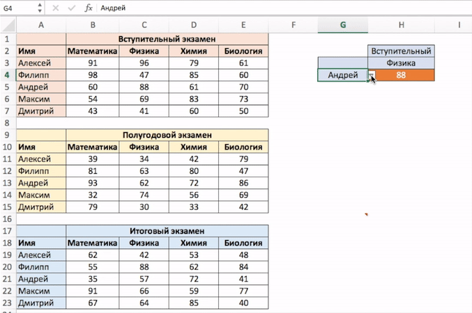
Функция INDEX (ИНДЕКС) в Excel используется для получения данных из таблицы, при условии что вы знаете номер строки и столбца, в котором эти данные находятся.
Например, в таблице ниже, вы можете использовать эту функцию для того, чтобы получить результаты экзамена по Физике у Андрея, зная номер строки и столбца, в которых эти данные находятся.

Содержание
- Что возвращает функция
- Синтаксис
- Аргументы функции
- Дополнительная информация
- Примеры использования функции ИНДЕКС в Excel
- Пример 1. Ищем результаты экзамена по физике для Алексея
- Пример 2. Создаем динамический поиск значений с использованием функций ИНДЕКС и ПОИСКПОЗ
- Пример 3. Создаем динамический поиск значений с использованием функций INDEX (ИНДЕКС) и MATCH (ПОИСКПОЗ) и выпадающего списка
- Пример 4. Использование трехстороннего поиска с помощью INDEX (ИНДЕКС) / MATCH (ПОИСКПОЗ)
Что возвращает функция
Возвращает данные из конкретной строки и столбца табличных данных.
Синтаксис
=INDEX (array, row_num, [col_num]) — английская версия
=INDEX (array, row_num, [col_num], [area_num]) — английская версия
=ИНДЕКС(массив; номер_строки; [номер_столбца]) — русская версия
=ИНДЕКС(ссылка; номер_строки; [номер_столбца]; [номер_области]) — русская версия
Аргументы функции
- array (массив) — диапазон ячеек или массив данных для поиска;
- row_num (номер_строки) — номер строки, в которой находятся искомые данные;
- [col_num] ([номер_столбца]) (необязательный аргумент) — номер колонки, в которой находятся искомые данные. Этот аргумент необязательный. Но если в аргументах функции не указаны критерии для row_num (номер_строки), необходимо указать аргумент col_num (номер_столбца);
- [area_num] ([номер_области]) — (необязательный аргумент) — если аргумент массива состоит из нескольких диапазонов, то это число будет использоваться для выбора всех диапазонов.
Дополнительная информация
- Если номер строки или колонки равен “0”, то функция возвращает данные всей строки или колонки;
- Если функция используется перед ссылкой на ячейку (например, A1), она возвращает ссылку на ячейку вместо значения (см. примеры ниже);
- Чаще всего INDEX (ИНДЕКС) используется совместно с функцией MATCH (ПОИСКПОЗ);
- В отличие от функции VLOOKUP (ВПР), функция INDEX (ИНДЕКС) может возвращать данные как справа от искомого значения, так и слева;
- Функция используется в двух формах — Массива данных и Формы ссылки на данные:
— Форма «Массива» используется когда вы хотите найти значения, основанные на конкретных номерах строк и столбцов таблицы;
— Форма «Ссылок на данные» используется при поиске значений в нескольких таблицах (используете аргумент [area_num] ([номер_области]) для выбора таблицы и только потом сориентируете функцию по номеру строки и столбца.
Примеры использования функции ИНДЕКС в Excel
Пример 1. Ищем результаты экзамена по физике для Алексея
Предположим, у вас есть результаты экзаменов в табличном виде по нескольким студентам:
Для того, чтобы найти результаты экзамена по физике для Андрея нам нужна формула:
=INDEX($B$3:$E$9,3,2) — английская версия
=ИНДЕКС($B$3:$E$9;3;2) — русская версия
В формуле мы определили аргумент диапазона данных, где мы будем искать данные $B$3:$E$9. Затем, указали номер строки “3”, в которой находятся результаты экзамена для Андрея, и номер колонки “2”, где находятся результаты экзамена именно по физике.
Пример 2. Создаем динамический поиск значений с использованием функций ИНДЕКС и ПОИСКПОЗ
Не всегда есть возможность указать номера строки и столбца вручную. У вас может быть огромная таблица данных, отображение данных которой вы можете сделать динамическим, чтобы функция автоматически идентифицировала имя или экзамен, указанные в ячейках, и дала правильный результат.
Пример динамического отображения данных ниже:

Для динамического отображения данных мы используем комбинацию функций INDEX (ИНДЕКС) и MATCH (ПОИСКПОЗ).
Вот такая формула поможет нам добиться результата:
=INDEX($B$3:$E$9,MATCH($G$4,$A$3:$A$9,0),MATCH($H$3,$B$2:$E$2,0)) — английская версия
=ИНДЕКС($B$3:$E$9;ПОИСКПОЗ($G$4;$A$3:$A$9;0);ПОИСКПОЗ($H$3;$B$2:$E$2;0)) — русская версия
В формуле выше, не используя сложного программирования, мы с помощью функции MATCH (ПОИСКПОЗ) сделали отображение данных динамическим.
Динамический отображение строки задается следующей частью формулы —
MATCH($G$4,$A$3:$A$9,0) — английская версия
ПОИСКПОЗ($G$4;$A$3:$A$9;0) — русская версия
Она сканирует имена студентов и определяет значение поиска ($G$4 в нашем случае). Затем она возвращает номер строки для поиска в наборе данных. Например, если значение поиска равно Алексей, функция вернет “1”, если это Максим, оно вернет “4” и так далее.
Динамическое отображение данных столбца задается следующей частью формулы —
MATCH($H$3,$B$2:$E$2,0) — английская версия
ПОИСКПОЗ($H$3;$B$2:$E$2;0) — русская версия
Она сканирует имена объектов и определяет значение поиска ($H$3 в нашем случае). Затем она возвращает номер столбца для поиска в наборе данных. Например, если значение поиска Математика, функция вернет “1”, если это Физика, функция вернет “2” и так далее.
Больше лайфхаков в нашем Telegram Подписаться
Пример 3. Создаем динамический поиск значений с использованием функций INDEX (ИНДЕКС) и MATCH (ПОИСКПОЗ) и выпадающего списка
На примере выше мы вручную вводили имена студентов и названия предметов. Вы можете сэкономить время на вводе данных, используя выпадающие списки. Это актуально, когда количество данных огромное.
Используя выпадающие списки, вам нужно просто выбрать из списка имя студента и функция автоматически найдет и подставит необходимые данные.
Пример ниже:

Используя такой подход, вы можете создать удобный дашборд, например для учителя. Ему не придется заниматься фильтрацией данных или прокруткой листа со студентами, для того чтобы найти результаты экзамена конкретного студента, достаточно просто выбрать имя и результаты динамически отразятся в лаконичной и удобной форме.
Для того, чтобы осуществить динамическую подстановку данных с использованием функций INDEX (ИНДЕКС) и MATCH (ПОИСКПОЗ) и выпадающего списка, мы используем ту же формулу, что в Примере 2:
=INDEX($B$3:$E$9,MATCH($G$4,$A$3:$A$9,0),MATCH($H$3,$B$2:$E$2,0)) — английская версия
=ИНДЕКС($B$3:$E$9;ПОИСКПОЗ($G$4;$A$3:$A$9;0);ПОИСКПОЗ($H$3;$B$2:$E$2;0)) — русская версия
Единственное отличие, от Примера 2, мы на месте ввода имени и предмета создадим выпадающие списки:
- Выбираем ячейку, в которой мы хотим отобразить выпадающий список с именами студентов;
- Кликаем на вкладку “Data” => Data Tools => Data Validation;
- В окне Data Validation на вкладке “Settings” в подразделе Allow выбираем “List”;
- В качестве Source нам нужно выбрать диапазон ячеек, в котором указаны имена студентов;
- Кликаем ОК
Теперь у вас есть выпадающий список с именами студентов в ячейке G5. Таким же образом вы можете создать выпадающий список с предметами.
Пример 4. Использование трехстороннего поиска с помощью INDEX (ИНДЕКС) / MATCH (ПОИСКПОЗ)
Функция INDEX (ИНДЕКС) может быть использована для обработки трехсторонних запросов.
Что такое трехсторонний поиск?
В приведенных выше примерах мы использовали одну таблицу с оценками для студентов по разным предметам. Это пример двунаправленного поиска, поскольку мы используем две переменные для получения оценки (имя студента и предмет).
Теперь предположим, что к концу года студент прошел три уровня экзаменов: «Вступительный», «Полугодовой» и «Итоговый экзамен».
Трехсторонний поиск — это возможность получить отметки студента по заданному предмету с указанным уровнем экзамена.
Вот пример трехстороннего поиска:
В приведенном выше примере, кроме выбора имени студента и названия предмета, вы также можете выбрать уровень экзамена. Основываясь на уровне экзамена, формула возвращает соответствующее значение из одной из трех таблиц.
Для таких расчетов нам поможет формула:
=INDEX(($B$3:$E$7,$B$11:$E$15,$B$19:$E$23),MATCH($G$4,$A$3:$A$7,0),MATCH($H$3,$B$2:$E$2,0),IF($H$2=»Вступительный»,1,IF($H$2=»Полугодовой»,2,3))) — английская версия
=ИНДЕКС(($B$3:$E$7;$B$11:$E$15;$B$19:$E$23);ПОИСКПОЗ($G$4;$A$3:$A$7;0);ПОИСКПОЗ($H$3;$B$2:$E$2;0); ЕСЛИ($H$2=»Вступительный»;1;ЕСЛИ($H$2=»Полугодовой»;2;3))) — русская версия
Давайте разберем эту формулу, чтобы понять, как она работает.
Эта формула принимает четыре аргумента. Функция INDEX (ИНДЕКС) — одна из тех функций в Excel, которая имеет более одного синтаксиса.
=INDEX (array, row_num, [col_num]) — английская версия
=INDEX (array, row_num, [col_num], [area_num]) — английская версия
=ИНДЕКС(массив; номер_строки; [номер_столбца]) — русская версия
=ИНДЕКС(ссылка; номер_строки; [номер_столбца]; [номер_области]) — русская версия
По всем вышеприведенным примерам мы использовали первый синтаксис, но для трехстороннего поиска нам нужно использовать второй синтаксис.
Рассмотрим каждую часть формулы на основе второго синтаксиса.
- array (массив) – ($B$3:$E$7,$B$11:$E$15,$B$19:$E$23):Вместо использования одного массива, в данном случае мы использовали три массива в круглых скобках.
- row_num (номер_строки) – MATCH($G$4,$A$3:$A$7,0): функция MATCH (ПОИСКПОЗ) используется для поиска имени студента для ячейки $G$4 из списка всех студентов.
- col_num (номер_столбца) – MATCH($H$3,$B$2:$E$2,0): функция MATCH (ПОИСКПОЗ) используется для поиска названия предмета для ячейки $H$3 из списка всех предметов.
- [area_num] ([номер_области]) – IF($H$2=”Вступительный”,1,IF($H$2=”Полугодовой”,2,3)): Значение номера области сообщает функции INDEX (ИНДЕКС), какой массив с данными выбрать. В этом примере у нас есть три массива в первом аргументе. Если вы выберете «Вступительный» из раскрывающегося меню, функция IF (ЕСЛИ) вернет значение “1”, а функция INDEX (ИНДЕКС) выберут 1-й массив из трех массивов ($B$3:$E$7).
Уверен, что теперь вы подробно изучили работу функции INDEX (ИНДЕКС) в Excel!
Excel INDEX Function (Examples + Video)
When to use Excel INDEX Function
Excel INDEX function can be used when you want to fetch the value from a tabular data and you have the row number and column number of the data point. For example, in the example below, you can use the INDEX function to get the marks of ‘Tom’ in Physics when you know the row number and the column number in the data set.
What it Returns
It returns the value from a table for the specified row number and column number.
Syntax
=INDEX (array, row_num, [col_num])
=INDEX (array, row_num, [col_num], [area_num])
INDEX function has 2 syntax. The first one is used in most cases, however, in case of three-way lookups, the second one is used (covered in Example 5).
Input Arguments
- array – a range of cells or an array constant.
- row_num – the row number from which the value is to be fetched.
- [col_num] – the column number from which the value is to be fetched. Although this is an optional argument, but if row_num is not provided, it needs to be given.
- [area_num] – (Optional) If array argument is made up of multiple ranges, this number would be used to select the reference from all the ranges.
Additional Notes (Boring Stuff.. But Important to Know)
- If the row number or the column number is 0, it returns the values of the entire row or column respectively.
- If INDEX function is used in front of a cell reference (such as A1:) it returns a cell reference instead of a value (see examples below).
- Most widely used along with the MATCH function.
- Unlike VLOOKUP, INDEX function can return a value from the left of the lookup value.
- INDEX function have two forms – Array form and the Reference form
- ‘Array form’ is where you fetch a value based on row and column number from a given table.
- ‘Reference form’ is where there are multiple tables, and you use the area_num argument to select the table and then fetch a value within it using the row and column number (see live example below).
Excel INDEX Function – Examples
Here are six examples of using Excel INDEX Function.
Example 1 – Finding Tom’s Marks in Physics (a two-way lookup)
Suppose you have a dataset as shown below:
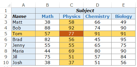
To find Tom’s marks in Physics, use the below formula:
=INDEX($B$3:$E$10,3,2)
This INDEX formula specifies the array as $B$3:$E$10 which has the marks for all the subjects. Then it uses the row number (3) and column number (2) to fetch Tom’s marks in Physics.
Example 2 – Making the LOOKUP Value Dynamic using MATCH Function
It may not always be possible to specify the row number and the column number manually. You may have a huge data set, or you may want to make it dynamic so that it automatically identifies the name and/or subject specified in cells and give the correct result.
Something as shown below:
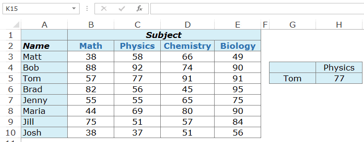
This can be done using a combination of the INDEX and the MATCH function.
Here is the formula that will make the lookup values dynamic:
=INDEX($B$3:$E$10,MATCH($G$5,$A$3:$A$10,0),MATCH($H$4,$B$2:$E$2,0))
In the above formula, instead of hard-coding the row number and the column number, MATCH function is used to make it dynamic.
- Dynamic Row Number is given by the following part of the formula – MATCH($G$5,$A$3:$A$10,0). It scans the name of students and identifies the lookup value ($G$5 in this case). It then returns the row number of the lookup value in the dataset. For example, if the lookup value is Matt, it’ll return 1, if it is Bob, it’ll return 2 and so on.
- Dynamic Column Number is given by the following part of the formula – MATCH($H$4,$B$2:$E$2,0). It scans the subject names and identifies the lookup value ($H$4 in this case). It then returns the column number of the lookup value in the dataset. For example, if the lookup value is Math, it’ll return 1, if it is Physics, it’ll return 2 and so on.
Example 3 – Using Drop Down Lists as Lookup Values
In the above example, we have to manually enter the data. That could be time-consuming and error-prone, especially if you have a huge list of lookup values.
A good idea in such cases is to create a drop down list of the lookup values (in this case, it could be student names and subjects) and then simply choose from the list. Based on the selection, the formula would automatically update the result.
Something as shown below:

This makes a good dashboard component as you can have a huge data set with hundreds of students at the back end, but the end user (let’s say a teacher) can quickly get the marks of a student in a subject by simply making the selections from the drop down.
How to make this:
The formula used in this case is the same used in Example 2.
=INDEX($B$3:$E$10,MATCH($G$5,$A$3:$A$10,0),MATCH($H$4,$B$2:$E$2,0))
The lookup values have been converted into drop-down lists.
Here are the steps to create the Excel drop down list:
- Select the cell in which you want the drop-down list. In this example, in G4, we want the student names.
- Go to Data –> Data Tools –> Data Validation.
- In the Data Validation Dialogue box, within the settings tab, select List from the Allow drop-down.
- In the source, select $A$3:$A$10
- Click OK.
Now you’ll have the drop-down list in cell G5. Similarly, you can create one in H4 for the subjects.
Example 4 – Return Values from an Entire Row/Column
In the above examples, we’ve used Excel INDEX function to do a 2-way lookup and get a single value.
Now, what if you want to get all the marks of a student. This can enable you to find the maximum/minimum score of that student, or the total marks scored in all subjects.
In simple English, you want to first get the entire row of scores for a student (let’s say Bob) and then within those values identify the highest score or the total of all the scores.
Here is the trick.
In Excel INDEX Function, when you enter the column number as 0, it will return the values of that entire row.
So the formula for this would be:
=INDEX($B$3:$E$10,MATCH($G$5,$A$3:$A$10,0),0)
Now this formula. if used as is, would return the #VALUE! error. While it displays the error, in the backend, it returns an array that has all the scores for Tom – {57,77,91,91}.
If you select the formula in the edit mode and press F9, you’ll be able to see the array it returns (as shown below): 
Similarly, based on what the lookup value is, when the column number is specified as 0 (or is left blank), it returns all the values in the row for the lookup value
Now to calculate the total score obtained by Tom, we can simply use the above formula within the SUM function.
=SUM(INDEX($B$3:$E$10,MATCH($G$5,$A$3:$A$10,0),0))
On similar lines, to calculate the highest score, we can use MAX/LARGE and to calculate minimum, we can use MIN/SMALL.

Example 5 – Three Way Lookup Using INDEX/MATCH
Excel INDEX function is built to handle three-way lookups.
What is a three-way lookup?
In the above examples, we’ve used one table with scores for students in different subjects. This is an example of a two-way lookup as we use two variables to fetch the score (student’s name and the subject).
Now, suppose in a year, a student has three different levels of exams, Unit Test, Midterm, and Final Examination (that’s what I had when I was a student).
A three-way lookup would be the ability to get a student’s marks for a specified subject from the specified level of exam. This would make it a three-way lookup as there are three variables (student’s name, subject’s name, and the level of examination).
Here is an example of a three-way lookup:
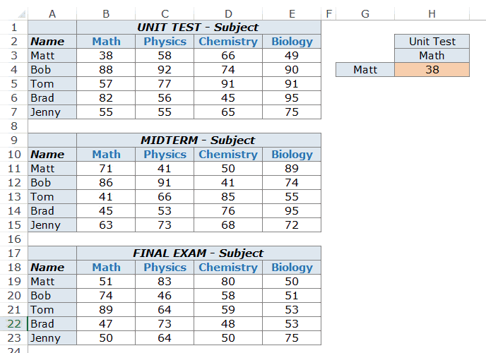
In the example above, apart from selecting the student’s name and subject name, you can also select the level of exam. Based on the level of exam, it returns the matching value from one of the three tables.
Here is the formula used in cell H4:
=INDEX(($B$3:$E$7,$B$11:$E$15,$B$19:$E$23),MATCH($G$4,$A$3:$A$7,0),MATCH($H$3,$B$2:$E$2,0),IF($H$2="Unit Test",1,IF($H$2="Midterm",2,3)))
Let’s break down this formula to understand how it works.
This formula takes four arguments. INDEX is one of those functions in Excel that has more than one syntax.
=INDEX (array, row_num, [col_num])
=INDEX (array, row_num, [col_num], [area_num])
So far in all the example above, we have used the first syntax, but to do a three-way lookup, we need to use the second syntax.
Now let’s see each part of the formula based on the second syntax.
- array – ($B$3:$E$7,$B$11:$E$15,$B$19:$E$23): Instead of using a single array, in this case, we have used three arrays within parenthesis.
- row_num – MATCH($G$4,$A$3:$A$7,0): MATCH function is used to find the position of the student’s name in cell $G$4 in the list of student’s name.
- col_num – MATCH($H$3,$B$2:$E$2,0): MATCH function is used to find the position of the subject name in cell $H$3 in the list of subject’s name.
- [area_num] – IF($H$2=”Unit Test”,1,IF($H$2=”Midterm”,2,3)): The area number value tells the INDEX function which array to select. In this example, we have three arrays in the first argument. If you select Unit Test from the drop-down, the IF function returns 1 and the INDEX functions select 1st array from the three arrays (which is $B$3:$E$7).
Example 6 – Creating a Reference Using the INDEX Function (Dynamic Named Ranges)
This is one wild use of the Excel INDEX function.
Let’s take a simple example.
I have a list of names as shown below:

Now I can use a simple INDEX function to get the last name on the list.
Here is the formula:
=INDEX($A$2:$A$9,COUNTA($A$2:$A$9))
This function simply counts the number of cells that are not empty and returns the last item from this list (it works only when there are no blanks in the list).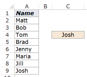
Now, what here comes the magic.
If you put the formula in front of a cell reference, the formula would return a cell reference of the matching value (instead of the value itself).
=A2:INDEX($A$2:$A$9,COUNTA($A$2:$A$9))
You would expect the above formula to return =A2:”Josh” (where Josh is the last value in the list). However, it returns =A2:A9 and hence you get an array of names as shown below:
One practical example where this technique can be helpful is in creating dynamic named ranges.
That’s it in this tutorial. I’ve tried to cover major examples of using the Excel INDEX function. If you would like to see more examples added to this list, let me know in the comments section.
Note: I’ve tried my best to proof read this tutorial, but in case you find any errors or spelling mistakes, please let me know 🙂
Excel INDEX Function – Video Tutorial
Related Excel Functions:
- Excel VLOOKUP Function.
- Excel HLOOKUP Function.
- Excel INDIRECT Function.
- Excel MATCH Function.
- Excel OFFSET Function.
You May Also Like the Following Excel Tutorials:
- VLOOKUP Vs. INDEX/MATCH
- Excel Index Match
- Lookup and Return Values in an Entire Row/Column.
The Excel INDEX function can lookup a range of cells and return any of the following:
- a single value
- an array of values
- a reference to a cell
- a reference to a range of cells.
It’s this flexibility that makes it a truly powerful function, even if you only use it for the first option.
We’ll start with some straight forward examples and build from there, but first, the technicalities.
| Syntax 1: | =INDEX( array, row_num, [column_num]) |
Excel INDEX Function Arguments
I’ll say this now, but don’t worry if it doesn’t resonate yet because I’ll show you an example later:
If the array has more than one row and more than one column, and only row_num or column_num is used, then INDEX will return an array of the entire row or column in the array argument.
Download the Workbook and Follow Along
Enter your email address below to download the sample workbook.
By submitting your email address you agree that we can email you our Excel newsletter.
Excel INDEX Function Examples
We’ll start with a basic data table to use in the examples:
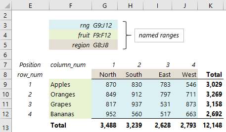
Note that the row labels, column headers and values areas all have named ranges which I’ll use in the formula examples. I’ve also added a total row and column, so you can cross reference the formula results to aid understanding.
INDEX Function Examples
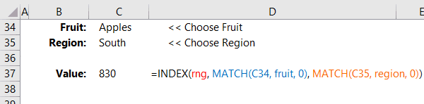
Perhaps the most common use of the INDEX function is to lookup a value in a range (which is the array argument), and return a value from the corresponding row/column intersection. For example, let’s say I want to know the value for Grapes in the West region.
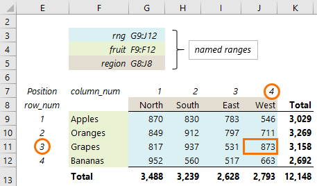
I could use this INDEX formula:
=INDEX(rng, 3, 4)
In English is reads, lookup the cells called ‘rng’ and return the value that at the intersection of row number 3, and column number 4.
=873
But if we already know that Grapes is in row 3 and West is in column 4, then we don’t really need INDEX, do we?
No, the real power comes when you use MATCH to find the row_num and column_num arguments like this:
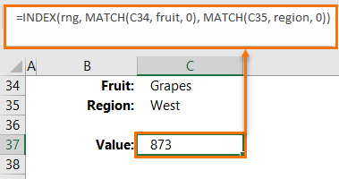
Formula in cell C37:
=INDEX(rng, MATCH(C34, fruit, 0), MATCH(C35, region, 0))
In English the above formula reads; lookup the rng and return the value at the intersection of the row that matches ‘Grapes’ in the ‘fruit’ range and the column that matches ‘West’ in the ‘region’ range.
Which evaluates to this:
=INDEX(rng, 3, 4)
=873
Note: If the row_num or column_num points to a cell outside of the array, INDEX will return the #REF! error.
Now that MATCH is doing the heavy lifting we can really put it to work with data validation lists that allow us to toggle through the different items like this:
Congratulations, you’ve just mastered INDEX & MATCH as an alternative to VLOOKUP.
More on the Excel MATCH function.
INDEX Single Row or Column
In certain circumstances the INDEX function’s row_num and column_num arguments are optional, namely:
If the array being indexed only contains a single column then there is no need for the column_num argument.
Obviously, you might say, but stick with me, there’s a twist.
For example, let’s say we want to return the value in row number 2 of the Fruit range.
We can simply write the formula like this:
=INDEX( fruit, 2)
=Oranges
Likewise, if the array being indexed only contains a single row, there is no need for the row_num argument.
For example, let’s say we want to return the value in column number 3 of the Region range (cells G8:J8).
We can write the formula like this:
=INDEX(region, 3)
=East
Hold up! Did you notice the column_num argument, 3, is in the row_num argument’s position?
If you prefer to use a placeholder for the row_num argument you can add a comma to your INDEX formula like this:
=INDEX(region, , 3)
But, this extra comma is not strictly necessary as INDEX is looking up the array provided and returning the value in the third position, irrespective of whether the array is arranged in a row or column.
In other words, if your array is a single dimension, either a row or a column, then only one more argument is required for the position you want returned. And that argument can be placed in the row_num or column_num position of the formula.
But that’s not all folks, you can also write the formula like this:
=INDEX(region, 1, 3)
Of course, telling INDEX to return a value from row 1 of a single row array is an insult to its intelligence 😉.
Another option is to use zero for the row_num argument, like this:
=INDEX(region, 0, 3)
What? Row zero. Where is that? Well, when the row_num argument is zero, or empty, INDEX actually returns a reference to the whole column specified by the column_num argument. In this case the whole column is only 1 row high, or in other words, one cell; I8.
The inverse of this also applies; i.e. if your array is a column and you omit or use zero for the column_num argument.
Now, if you learn nothing more than the above points you’ll be way ahead of most Excel users. So, well done.
However, if you haven’t learnt anything new so far, or you’re eager to learn more, then keep reading because we’re going to start looking at the other 3 things the Excel INDEX function can do.
Return a Range with Excel INDEX Function
Expanding on the idea of omitting arguments or using zero for the row or column num arguments, let’s take a look at what happens when we reference the rng array.
I’ll repeat my earlier point; when a row or column num argument is omitted, or zero is used, INDEX actually returns a reference to the whole row or column.
However, typically INDEX is placed in a single cell and so when the range being returned is more than one cell, INDEX will return the #VALUE! error.
Let me illustrate these points with the following formula, which returns the second column of the cells named ‘rng’:
=INDEX(rng, ,2)
In other words, the above formula returns the range H9:H12.
There are 3 examples of this range being returned by INDEX in the image below:
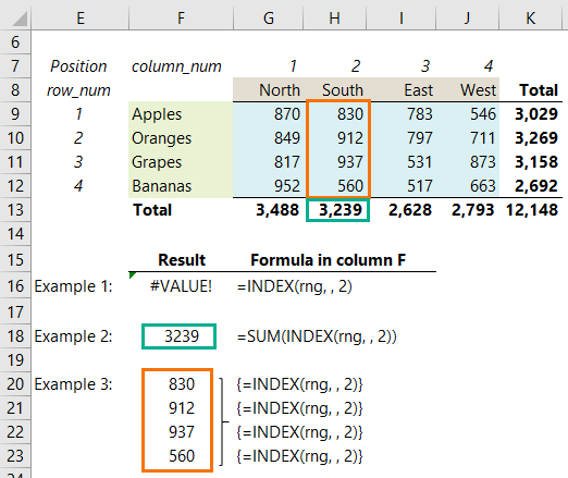
Example 1: Cell F16 — INDEX is entered in a single cell and returns the #VALUE! error. It’s returning the range H9:H12 and we haven’t told Excel what to do with that range, so #VALUE! is returned. We’d get the same error if we simply entered = H9:H12 into a cell.
Example 2: Cell F18 – INDEX is wrapped in the SUM function and returns the sum of the range H9:H12. It’s the same as entering =SUM(H9:H12) into a cell.
Example 3: Cells F20:F23 – INDEX has been array entered* into 4 cells which enables it to return the 4 values.
*To ‘array enter’ this formula, select the 4 cells (because the range H9:H12 is 4 cells high), then type the formula in and press CTRL+SHIFT+ENTER to complete the formula. This inserts the curly braces around the formula that you can see in the screenshot above, and places the 4 values in individual cells.
Notes:
- When you array enter the formula in example 1 (with CTRL+SHIFT+ENTER), it will return the first value in the range, i.e. 830.
- If you enter the formula in example 1 on rows 9, 10, 11 or 12, it will return the value on the corresponding row, as opposed to the #VALUE! error. This is due to implicit intersection.
Uses for INDEX Returning a Range
Extending what we know about INDEX being able to return a range, let’s look at some uses for this with a new data set shown below. Note the new named ranges; sales, dept and period.
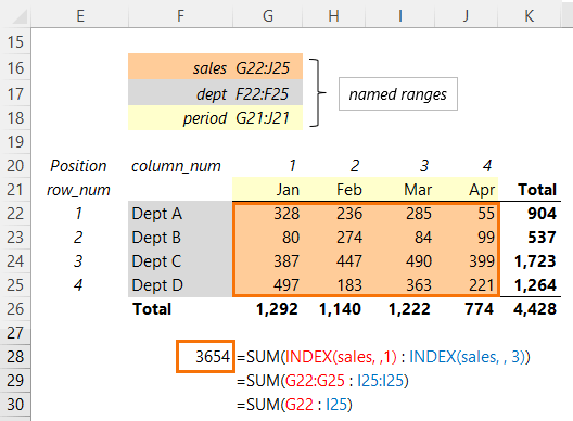
In cell F28 in the image above we can see the range being summed is returned by an INDEX formula on either side of the colon operator:
=SUM(INDEX(sales, ,1) : INDEX(sales, , 3))
It evaluates like so:
=SUM(G22:G25 : I22:I25)
In the next evaluation step Excel only keeps the extremities of the two ranges so we end up with:
=SUM(G22 : I25)
=3654
Now consider making the periods being summed dynamic. We can do this by replacing the column_num arguments with references to another cell that contains data validation lists that the user can choose from:
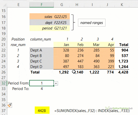
Most people use the OFFSET function to calculate dynamic named ranges, but INDEX is far more efficient and doesn’t suffer the volatility of OFFSET.
Excel INDEX Function – 4 Uses
Circling back to the 4 uses for INDEX, which were to return:
- a single value
- an array of values
- a reference to a cell
- a reference to a range of cells.
Have you made the connection that 1 and 3 are the same thing, and 2 and 4 are the same thing? And whether you get a value/values or a reference simply depends on how you use INDEX.
For example, the following formula:
=INDEX(sales, 1, 1)
Returns the reference to cell G22:
If you enter the above formula in an empty cell it will display the value from cell G22; which is 328.
But if you enter this INDEX formula nested in another formula, it will return the cell reference.
=COUNT(INDEX(sales, 1,1))
=COUNT(G22)
=1
More on dynamic named ranges here.
Referencing Non-contiguous Ranges
You may have noticed that INDEX has two syntax options:
The first one returns an array (single or multiple values), and the other returns a reference to a cell, or range of cells.
You don’t actually choose which syntax to use, Excel will decide that based on the inputs and the context of the formula. For example; whether the formula is entered in a single cell, nested inside another function, array entered etc.
So far, we’ve covered scenarios where the array or reference is a single contiguous range. So, let’s look at the second one which allows you to work with non-contiguous ranges.
Excel INDEX Function Syntax – Non-contiguous Ranges
| Syntax 2: | =INDEX( reference, row_num, [column_num], [area_num]) |
*References must be on the same sheet, otherwise the #VALUE! error is returned. References can be different shapes/sizes, but if the row_num or column_num argument refers to a row or column outside of the reference area, INDEX will return the #REF! error.
INDEX Non-contiguous Range Examples
In the screenshot below we have two sets of stores; Stores A to D and Stores E to H. Just imagine there are two managers responsible for these two store groups and that’s the reason for their separation.
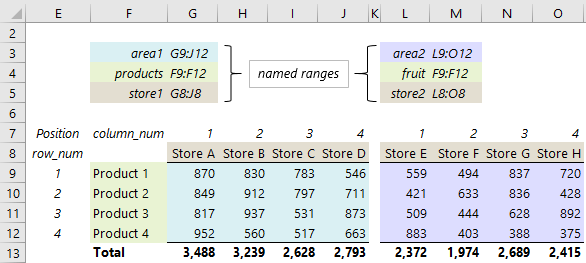
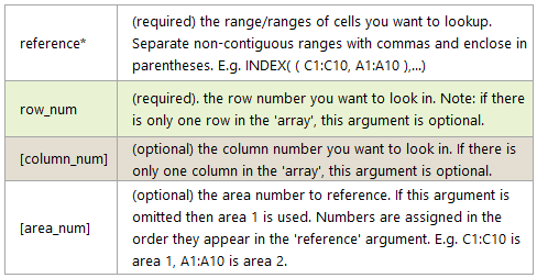
Let’s say we want to find the value for Product 4 in Store G. We’d use this INDEX formula:
=INDEX((area1, area2), 4, 3, 2)
=388
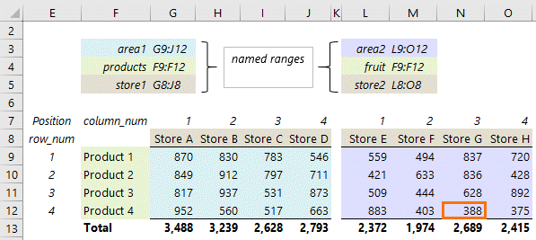
Notice the two references are separated by a comma and wrapped in parentheses:
=INDEX( (area1, area2), 4, 3, 2)
Remember, the references must be on the same sheet, otherwise INDEX will return the #VALUE! error.
Reference a Whole Column or Row
We can also return a reference to a whole row or column. For example, if I want to sum the values for store G, I can put a zero in the row_num argument like this:
=SUM(INDEX((area1, area2), 0, 3, 2))
=2,689
And I can sum Product 4 for Area 1 like this:
=SUM(INDEX((area1, area2), 4, 0, 1))
=2,692
Notice that it doesn’t sum all of Product 4, only that of area 1.
Excel INDEX Function Limitations
It’s such a versatile function and there aren’t many limitations. Perhaps the main limitation is the requirement that the reference ranges must be on the same sheet. The workaround to this is to use a different function to return the reference.
The Excel CHOOSE function is a great alternative:
=SUM( INDEX( CHOOSE( 1, area1, area2), 4, 0) )
=SUM( INDEX( area1, 4, 0) )
=2,692
Notice that instead of this:
=SUM(INDEX((area1, area2), 4, 0, 1))
We have this:
=SUM( INDEX( CHOOSE( 1, area1, area2), 4, 0) )
Related Functions
| MATCH Function | The MATCH function looks up a value in a range and returns the relative position of that value. |
| OFFSET Function | The OFFSET Function returns a range of cells offset from a starting cell. |
| Dynamic Named Ranges | Dynamic named ranges automatically update based on criteria you specify. |
| CHOOSE Function | The CHOOSE Function returns a value or range from a list based on the position specified. |
| VLOOKUP Function | The VLOOKUP function looks up a value in a column and returns a corresponding value from a column to the right. |
| HLOOKUP Function | The HLOOKUP function looks up a value in a row and returns a corresponding value from a row below. |
Excel INDEX Function Formula Examples
INDEX & MATCH
Excel Lookup Multiple Sheets
Dynamic Dependent Data Validation
Excel Find Column Containing a Value
INDEX and MATCH Two Criteria
Return the First and Last Values in a Range
Locating Values in Large Excel Tables
Excel Remove Blank Cells from a Range
Lookup and Return Multiple Matches
Search a Cell for a List of Words
Hyperlink Triptych
Cool INDEX Function Trick
Excel Dynamic Text Labels
Lookup Multiple Values in Multiple Columns
In this article I will explain the INDEX() function in Excel. Basically this function receives a range of cells, a row index and a column index as input. It returns the the value or reference of the cell at the specified row and column index.
Jump To:
- Syntax
- Example 1
- Example 2
- Example 3
- Example 4
Syntax:
=INDEX(Range, row_Index, column_Index, Area)
Range: A range of cells
row_Index: The row index of the cell value or reference desired. Note this is the row index relative to the range.
column_Index: The column index of the cell value or referenced desired. Note this is the column index relative to the range.
Area: In case multiple ranges have been chosen, this parameter selects which range is intended.
Example 1:
=Index(E1:G3, 2, 3)

Result: The value in the the second row, third column (column G) of the table is returned

You can download the workbook for example 1 and 2 here.
–
Example 2:
=Index(F3:G5, 3, 2)

Result: The value in the the third row (row 5), second column (column G) of the table is returned:

You can download the workbook for example 1 and 2 here.
–
Example 3:
In this example it is assumed we have a database of information on sheet2.
Database in sheet2:

On cell A2 of sheet1 the user will input a row index. Based on the row index selected selected the values in cells C2, D2, E2 and F2 are updated. In the figure below the user has selected the row index 4. The row index 4 corresponds to the name “Emma”, age “30”, account balance “$12,484.00” and account number “1654567”:

In the figure below the user has input “2” in cell A2. The row index 2 corresponds to the name “John”, age “50”, account balance “$85,541.00” and account number “1654565”:

Below you can see the formulas used in each cell:

Cell C2: The formula used in this cell is:
=INDEX(Sheet2!A2:A9, $A2, 1)
Sheet2!A2:A9:The range in Sheet2 with the names in it:

$A2: The cell where the row index is input by the user:

“1”: The column index in the range Sheet2!A2:A9 to retrieve the value from. Note that the range Sheet2!A2:A9 only has 1 column therefore the column index could have been omitted. The formula below would have returned the same value:
=INDEX(Sheet2!A2:A9, $A2)
Cell D2: Similar to cell C2. The input range (=INDEX(Sheet2!B2:B9, $A2, 1)) is the second column in sheet2 (the range with the ages in it):

The rest of the parameters are the same as cell C2.
Cell E2: Similar to cell C2. The input range (=INDEX(Sheet2!C2:C9, $A2, 1)) is the third column in sheet2 (the range with the Account Balances in it):

The rest of the parameters are the same as cell C2.
Cell F2: Similar to cell C2. The input range(=INDEX(Sheet2!D2:D9, $A2, 1)) is the third column in sheet2 (the range with the Account Numbers in it):

The rest of the parameters are the same as cell C2. You can download the workbook for example 3 here.
–
Example 4:
In this example it is assumed we have the following data in sheet2:

As you can see in the figure above, in column B there are payment values and in column B there is the date when each payment was made. What we want to do, is to be able to choose a starting and ending row index, and to find the total sum of payments made between those 2 rows:

The value 221$ displayed in cell B3 in the figure above is equivalent to the sum of the cells B2 to B5 in sheet2:

By changing the values in cells B1 and B2 of Sheet1, the value in cell B3 will be updated accordingly:

By changing cell B1 to 3 and B2 to 9 in the figure above, cell B3 will show the sum of the cells below:
 Probably wondering how this was done. This can be achieved by using the formula below in cell B3 in sheet1:
=SUM(INDEX(Sheet2!B2:B10, B1, 1):INDEX(Sheet2!B2:B10,B2, 1))
The syntax for the SUM function is:
=SUM(Cell1:Cell2)
So basically instead of Cell1 I’ve used:
INDEX(Sheet2!B2:B10, B1, 1)
and instead of Cell2 I’ve used:
INDEX(Sheet2!B2:B10, B2, 1)
As you can see in this example the INDEX function is returning a reference to a cell rather than the cell value as in the previous examples.
Sheet2!B2:B10: The range which the payments are located in:
=SUM(INDEX(Sheet2!B2:B10, B1, 1):INDEX(Sheet2!B2:B10,B2, 1))
B2 and B1: References to the values in cells B1 and B2 in sheet1. They contain the row index of the cell which the INDEX() function is supposed to return a reference to:
=SUM(INDEX(Sheet2!B2:B10, B1, 1):INDEX(Sheet2!B2:B10,B2, 1))
The number “1”: The column INDEX from which the INDEX function is supposed to return the cell reference from. Since the input range has only one column, the number “1” could have been omitted from the input parameters.
For the first example above where B1 = 1 and B2 = 4 the formula
=SUM(INDEX(Sheet2!B2:B10, B1, 1):INDEX(Sheet2!B2:B10,B2, 1))
would be equivalent to:
=SUM(Sheet2!B2:Sheet2!B5)
and for the second example where B1 = 3 and B2 = 9 the formula
=SUM(INDEX(Sheet2!B2:B10, B1, 1):INDEX(Sheet2!B2:B10,B2, 1))
would be equivalent to:
=SUM(Sheet2!B4:Sheet2!B10)
You can download the workbook for example 4 here.
See also:
- Excel VLOOKUP vs INDEX and MATCH Speed Comparison
- Excel INDEX MATCH Functions
- Excel, MATCH() function
If you need assistance with your code, or you are looking to hire a VBA programmer feel free to contact me. Also please visit my website www.software-solutions-online.com
Skip to content
В этом руководстве вы найдете ряд примеров формул, демонстрирующих наиболее эффективное использование ИНДЕКС в Excel.
Из всех функций Excel, возможности которых часто недооцениваются и используются недостаточно, ИНДЕКС определенно занимает место в первой десятке. Между тем, эта функция умна, гибка и универсальна.
Итак, что такое функция ИНДЕКС в Excel? По сути, формула ИНДЕКС (в английской версии – INDEX) возвращает ссылку на ячейку из заданного массива или диапазона. Другими словами, вы используете её, когда знаете (или можете определить) положение элемента в диапазоне и хотите затем получить значение этого элемента.
- Синтаксис и способы использования
- Получение N-го элемента из списка
- Получение всех значений в строке или столбце
- Использование ИНДЕКС с другими функциями (СУММ, СРЗНАЧ, МАКС, МИН)
- Формула ИНДЕКС для создания динамических диапазонов и раскрывающихся списков
- Мощный поиск с ИНДЕКС/ПОИСКПОЗ
- Формула ИНДЕКС для получения одного диапазона из списка диапазонов
Если вы оцените реальный потенциал функции ИНДЕКС, это может кардинально изменить способы расчета, анализа и представления данных в ваших таблицах.
Функция ИНДЕКС в Excel — синтаксис и основные способы использования
В Excel есть две версии функции ИНДЕКС — форма массива и форма ссылки. Обе их можно использовать во всех версиях Microsoft Excel 365, 2019, 2016, 2013, 2010, 2007 и 2003.
Форма массива ИНДЕКС
В данном случае функция ИНДЕКС возвращает значение элемента в таблице или массиве на основе указанных вами номеров строк и столбцов.
ИНДЕКС(массив,номер_строки,[номер_столбца])
- массив — это диапазон ячеек, именованный диапазон или таблица.
- Номер_строки — это номер строки в массиве, из которого нужно вернуть значение. Если этот аргумент опущен, требуется следующий – номер_столбца.
- Номер_столбца — это номер столбца, из которого нужно вернуть значение. Если он опущен, требуется номер_строки.
Например, формула =ИНДЕКС(C2:F11;4;3) возвращает значение на пересечении четвертой строки и третьего столбца в диапазоне C2:F11, что является значением в ячейке D4.
Чтобы получить представление о том, как формула ИНДЕКС работает с реальными данными, взгляните на следующий пример:

Вместо того, чтобы вводить в формулу номера строк и столбцов, вы можете указать ссылки на ячейки, чтобы получить более универсальную формулу:
=ИНДЕКС(C2:F11;I1;I2)
Итак, эта формула ИНДЕКС возвращает количество товаров точно на пересечении номера товара, указанного в ячейке I1 (номер_строки), и номера недели, введенного в ячейке I2 (номер_столбца).
Примечание. Использование абсолютных ссылок ($C$2:$F$11) вместо относительных ссылок (C2:F11) в аргументе массива упрощает копирование формулы в другие ячейки. Кроме того, вы можете преобразовать диапазон в таблицу (Ctrl + Т) и обращаться к нему по имени таблицы.
Что нужно помнить
- Если аргумент массива состоит только из одной строки или столбца, вы можете указать или не указать соответствующий аргумент номер_строки или номер_столбца.
- Если аргумент массива включает более одной строки, а номер_строки опущен или равен 0, функция ИНДЕКС возвращает массив всего столбца. Точно так же, если массив включает более одного столбца, а аргумент номер_столбца опущен или равен 0, формула ИНДЕКС возвращает всю строку. Вот пример формулы, демонстрирующий такое поведение.
- Аргументы номер_строки и номер_столбца должны ссылаться на ячейку в массиве; в противном случае формула ИНДЕКС вернет ошибку #ССЫЛКА!.
Форма ИНДЕКС в виде ссылки
Ссылочная форма функции ИНДЕКС Excel возвращает ссылку на ячейку на пересечении указанной строки и столбца.
ИНДЕКС(ссылка, номер_строки, [номер_столбца], [номер_области] )
- ссылка — это один или несколько диапазонов.
Если вы вводите более одного диапазона, разделите диапазоны точкой с запятой и заключите аргумент ссылки в круглые скобки, например (A1:B5; D1:F5).
Если каждый диапазон в ссылке содержит только одну строку или столбец, соответствующий аргумент номер_строки или номер_столбца является необязательным.
- номер_строки – порядковый номер строки в диапазоне, из которого возвращается ссылка на ячейку, аналогично форме массива.
- номер_столбца — порядковый номер столбца, из которого возвращается ссылка на ячейку, также работает аналогично форме массива.
- номер_области — необязательный параметр, указывающий, какой диапазон из ссылочного аргумента использовать. Если он не указан, формула ИНДЕКС вернет результат для первого диапазона, указанного в ссылке.
Например, формула =ИНДЕКС((B2:F4;B8:F11);3;2;2) возвращает значение ячейки С10, которая находится на пересечении 3-й строки и 2-го столбца во второй области (B8:F11).

Что нужно помнить о функции ИНДЕКС в форме ссылки
- Если аргумент номер_строки или номер_столбца равен нулю (0), формула ИНДЕКС возвращает ссылку для всего столбца или строки соответственно.
- Если и номер_строки, и номер_столбца опущены, функция ИНДЕКС возвращает область, указанную в аргументе номер_области.
- Все аргументы (номер_строки, номер_столбца и номер_области) должны ссылаться на ячейку в пределах заданного диапазона. В противном случае формула ИНДЕКС вернет ошибку #ССЫЛКА!
Обе формулы ИНДЕКС, которые мы обсуждали до сих пор, очень просты и служат только для иллюстрации. Ваши реальные формулы, вероятно, будут намного сложнее. Поэтому давайте рассмотрим несколько наиболее эффективных способов использования ИНДЕКС в Excel.
Как использовать функцию ИНДЕКС в Excel — примеры формул
Возможно, сама по себе функция ИНДЕКС в Excel не имеет большого практического применения, но в сочетании с другими функциями, такими как ПОИСКПОЗ или СЧËТ, она может создавать очень мощные формулы.
Далее во всех наших формулах ИНДЕКС (кроме последней) мы будем использовать приведенные ниже данные.

1. Получение N-го элемента из списка
Это основное использование функции ИНДЕКС и простейшая её формула. Чтобы получить определенный элемент из списка, вы просто пишете: =ИНДЕКС(диапазон; n), где диапазон — это диапазон ячеек или именованный диапазон, а n — позиция элемента, который вы хотите из него получить.
Чтобы получить значение ячейки на пересечении определенной строки и столбца, вы используете тот же подход с той лишь разницей, что вы указываете и номер строки, и номер столбца. На самом деле, вы уже видели такую формулу в действии, когда мы обсуждали форму массива функции ИНДЕКС .
И вот еще один пример. В нашем образце таблицы, чтобы найти четвертую по величине планету в Солнечной системе, вы сортируете таблицу по столбцу Диаметр и используете следующую формулу ИНДЕКС:
=ИНДЕКС(A5:E13;4;1)
- A5:E13 — это ссылка на диапазон с данными.
- Номер_строки равен 4, потому что вы ищете четвертый элемент в списке,
- Номер_столбца равен 1, потому что мы хотим извлечь имя планеты.
Естественно, вы можете использовать ссылку на ячейку в аргументах номер_строки и/или номер_столбца, чтобы сделать вашу формулу более универсальной, как показано на скриншоте ниже:

Кроме того, вы можете не сортировать таблицу вручную, а сделать это при помощи формулы.
=ИНДЕКС(СОРТ(A5:E13;3;-1);B1;1)
Функция СОРТ сортирует таблицу по третьему столбцу в порядке убывания. Ну а затем ИНДЕКС делает всё остальное.
2. Получение всех значений в строке или столбце
Помимо извлечения одной ячейки, функция ИНДЕКС может возвращать массив значений из всей строки или столбца . Чтобы получить все значения из определенного столбца, вы должны опустить аргумент номер_строки или установить его равным 0. Аналогичным образом, чтобы получить всю строку, вы передаете пустое значение или 0 в номер_столбца.
Такие формулы ИНДЕКС вряд ли можно использовать сами по себе, потому что Excel не может уместить массив значений, возвращаемых формулой, в одну ячейку, и вы получите ошибку #ЗНАЧ!. Однако, если вы используете ИНДЕКС в сочетании с другими функциями, такими как СУММ или СРЗНАЧ, вы получите отличные результаты.
Например, вы можете использовать следующую формулу для расчета средней температуры планет в Солнечной системе:
=СРЗНАЧ(ИНДЕКС(A4:E12;;4))
В приведенной выше формуле аргумент номер_столбца равен 4, потому что температура находится в четвертом столбце нашей таблицы. Параметр номер_строки опущен.

Аналогичным образом можно найти минимальную и максимальную температуры:
=МИН(ИНДЕКС(A4:E12;;4))
=МАКС(ИНДЕКС(A4:E12;;4))
И посчитаем общую массу планет (масса – второй столбец в таблице):
=СУММ(ИНДЕКС(A4:E12;;2))
С практической точки зрения функция ИНДЕКС в приведенной выше формуле лишняя. Вы можете просто написать =СРЗНАЧ(D4:D12) и получить те же результаты.
При работе с реальными данными эта функция может оказаться полезной как часть более сложных формул, которые вы используете для анализа данных.
К примеру, формула =СУММ(ИНДЕКС(A4:E12;;С1)) позволит вам подсчитывать сумму в том столбце, номер которого вы укажете в ячейке C1.
3. Использование ИНДЕКС с другими функциями (СУММ, СРЗНАЧ, МАКС, МИН)
Из предыдущих примеров у вас может сложиться впечатление, что формула ИНДЕКС возвращает значения, но на самом деле она возвращает ссылку на ячейку, содержащую значение. И этот пример демонстрирует, как эту возвращаемую ссылку можно использовать.
Поскольку результат формулы ИНДЕКС является ссылкой, мы можем использовать его в других функциях для создания динамического диапазона. Звучит запутанно? Сейчас поясним.
Предположим, у вас есть формула =СРЗНАЧ(D4:D12), которая возвращает среднее значений в ячейках D4:D12. Вместо того, чтобы писать диапазон непосредственно в формуле, вы можете заменить либо D4, либо D12, либо их оба, функцией ИНДЕКС, например:
=СРЗНАЧ(D4 : ИНДЕКС(D1:D20,12))
Обе приведенные выше формулы дадут один и тот же результат, поскольку функция ИНДЕКС также возвращает ссылку на ячейку В12 (номер строки равен 12, номер столбца опущен). Разница в том, что диапазон формулы СРЗНАЧ / ИНДЕКС является динамическим, и как только вы измените аргумент номер_строки в ИНДЕКС, то диапазон, обрабатываемый функцией СРЗНАЧ, также изменится, и формула вернет другой результат.
По-видимому, такое использование формулы ИНДЕКС кажется слишком сложным и не всегда рациональным и логичным. Но этот подход имеет важное практическое применение, как показано в следующих примерах.
Пример 1. Вычислить среднее значение первых N элементов в списке
Допустим, вы хотите узнать средний диаметр N самых больших планет в солнечной системе.
Количество позиций, которые мы будем использовать для расчета, указываем в ячейке В1.
Затем вы сортируете таблицу по столбцу диаметра от наибольшего к наименьшему и используете следующую формулу расчёта среднего значения:
=СРЗНАЧ(C5:ИНДЕКС(C5:C13;B1))

Как видите, количество значений для расчета среднего мы можем выбирать, не корректируя саму формулу
Пример 2. Сумма элементов между указанными двумя элементами
Если вы хотите определить элементы верхней и нижней границы в своей формуле, вам просто нужно использовать две функции ИНДЕКС, чтобы вернуть первый и последний элемент, которые вам нужны.
Например, следующая формула при помощи функции СУММ возвращает сумму значений в столбце Масса между двумя элементами, указанными в ячейках B1 и Е1:
=СУММ(ИНДЕКС(B5:B13;B1):ИНДЕКС(B5:B13;E1))

4. Формула ИНДЕКС для создания динамических диапазонов и раскрывающихся списков
Как это часто бывает, когда вы начинаете упорядочивать данные на листе, вы можете не знать, сколько записей у вас в конечном итоге будет. Это не относится к нашей таблице планет, которая кажется полной, но кто знает…
В любом случае, если у вас есть изменяющееся количество элементов в данном столбце, скажем, от A1 до An , вы можете создать динамический именованный диапазон , включающий все ячейки с данными. При этом вы хотите, чтобы диапазон корректировался автоматически по мере добавления новых элементов или удаления некоторых из существующих. Например, если у вас сейчас 10 элементов, ваш именованный диапазон будет A1:A10. Если вы добавите новую запись, именованный диапазон автоматически расширится до A1:A11, а если вы передумаете и удалите эти вновь добавленные данные, диапазон автоматически вернется к A1:A10.
Основное преимущество этого подхода заключается в том, что вам не нужно постоянно обновлять все формулы в книге, чтобы убедиться, что они относятся к правильным диапазонам.
Одним из способов определения динамического диапазона является использование функции Excel СМЕЩ :
=СМЕЩ($A$2; 0; 0; СЧЁТЗ($A1:$A100)-1; 1)
Другим возможным решением является использование ИНДЕКС Excel вместе с СЧËТЗ:
=$A$2:ИНДЕКС($A2:$A100; СЧЁТЗ($A2:$A100))
В обеих формулах A2 — это ячейка, содержащая первый элемент списка. Динамический диапазон, создаваемый обеими формулами, будет идентичным.
Разница заключается в подходах. В то время как функция СМЕЩ перемещается от начальной точки на определенное количество строк и/или столбцов, то ИНДЕКС находит ячейку на пересечении определенной строки и столбца. Функция СЧËТЗ, используемая в обеих формулах, получает количество непустых ячеек в интересующем нас столбце.
В этом примере в столбце A 9 непустых ячеек, поэтому СЧËТЗ возвращает 9. Следовательно, ИНДЕКС возвращает $A$9, то есть последнюю использованную ячейку в столбце A (обычно ИНДЕКС возвращает значение, но в этой формуле оператор ссылки (:) заставляет его вернуть ссылку). И поскольку $A$1 является нашей отправной точкой, конечным результатом формулы будет диапазон $A$1:$A$9.
На следующем рисунке показано, как можно использовать такую формулу ИНДЕКС для создания динамического выпадающего списка.

Примечание. Самый простой способ создать динамически обновляемый выпадающий список — сделать именованный список на основе таблицы Excel. В этом случае вам не понадобятся сложные формулы, поскольку таблицы Excel сами по себе являются динамическими диапазонами.
Вы также можете использовать функцию ИНДЕКС для создания зависимых раскрывающихся списков, и в следующем руководстве объясняются все необходимые шаги: Создание каскадного раскрывающегося списка в Excel .
5. Мощный поиск с ИНДЕКС/ПОИСКПОЗ
Выполнение вертикального поиска — вот где функция ИНДЕКС действительно великолепна. Если вы когда-либо пробовали использовать функцию ВПР Excel , вы хорошо знаете ее многочисленные ограничения, такие как невозможность извлечения значений из столбцов слева от столбца поиска или ограничение в 255 символов для значения поиска.
Связка ИНДЕКС/ПОИСКПОЗ во многих отношениях превосходит ВПР:
- Никаких проблем с «левым» ВПР.
- Нет ограничений на размер искомого значения.
- Сортировка не требуется (ВПР с приблизительным совпадением требует сортировки столбца подстановки в порядке возрастания).
- Вы можете вставлять и удалять столбцы в таблице, не обновляя каждую связанную формулу.
- И последнее, но не менее важное: ИНДЕКС/ПОИСКПОЗ не замедляет работу Excel, как это происходит, если использовать несколько формул ВПР в большой таблице.
Вы используете ИНДЕКС / ПОИСКПОЗ следующим образом:
=ИНДЕКС ( столбец для возврата значения , (ПОИСКПОЗ ( искомое значение , столбец для поиска , 0))
Например, по коду заказа мы можем найти название товара. При этом функция ПОИСКПОЗ ищет совпадение с кодами заказа, а затем передает номер найденной позиции в функцию ИНДЕКС. Та же в свою очередь извлекает соответствующее значение из переданного ей диапазона.

Таким образом организуется так называемый «левый» поиск, когда нужно извлечь значение из столбца, находящегося слева от столбца поиска. Функция ВПР сделать это не может. Более подробно о «левом» поиске читайте в этой статье.
Дополнительные советы и примеры формул см. в руководстве по Excel ИНДЕКС/ПОИСКПОЗ .
6. Формула ИНДЕКС для получения одного диапазона из списка диапазонов
Еще одно умное и эффективное использование функции ИНДЕКС в Excel — это возможность получить один диапазон из списка диапазонов.
Предположим, у вас есть несколько списков (например, сведения о еженедельных продажах). Вы можете рассчитать среднее значение или суммировать значения в любом выбранном диапазоне с помощью одной формулы.
Вы можете использовать следующую формулу индекса для расчета суммы продаж в выбранном диапазоне:
=СУММ(ИНДЕКС((C2:C11;D2:D11;E2:E11;F2:F11);;;I1))
Обратите внимание, что сейчас мы используем функцию ИНДЕКС в виде ссылки. Число в последнем аргументе (номер_области) сообщает формуле, какой именно диапазон выбрать.
На скриншоте ниже для номера диапазона (ячейка I1) установлено значение 2. Поэтому формула вычисляет сумму продаж за вторую неделю. Выбран второй по счёту диапазон в списке – D2:D11.

Чтобы сделать формулу еще более удобной для пользователя, вы можете использовать проверку данных и создать в ячейке I2 выпадающий список с номерами недель, чтобы предотвратить ошибки и опечатки:

Вот несколько основных способов применения формулы ИНДЕКС в Excel.
Я надеюсь, что эти примеры показали вам, как использовать потенциал функции ИНДЕКС в ваших рабочих листах. Спасибо за чтение!