
Содержание
- How to Get the Sheet Name in Excel? Easy Formula
- Get Sheet Name Using the CELL Function
- Alternative Formula to Get Sheet Name (MID formula)
- Fetching Sheet Name and Adding Text to it
- Create a Sheet Index in Excel
- Assume that we have 5 Sheets
- Here comes a Code
- INDEX function in Excel — 6 most efficient uses
- Excel INDEX function — syntax and basic uses
- INDEX array form
- INDEX array form — things to remember
- INDEX reference form
- INDEX reference form — things to remember
- How to use INDEX function in Excel — formula examples
- Source data
- 1. Getting the N th item from the list
- 2. Getting all values in a row or column
- 3. Using INDEX with other functions (SUM, AVERAGE, MAX, MIN)
- Example 1. Calculate average of the top N items in the list
- Example 2. Sum items between the specified two items
- 4. INDEX formula to create dynamic ranges and drop-down lists
- 5. Powerful Vlookups with INDEX / MATCH
- 6. Excel INDEX formula to get 1 range from a list of ranges
How to Get the Sheet Name in Excel? Easy Formula
When working with Excel spreadsheets, sometimes you may have a need to get the name of the worksheet.
While you can always manually enter the sheet name, it won’t update in case the sheet name is changed.
So if you want to get the sheet name, so that it automatically updates when the name is changed, you can use a simple formula in Excel.
In this tutorial, I will show you how to get the sheet name in Excel using a simple formula.
This Tutorial Covers:
Get Sheet Name Using the CELL Function
CELL function in Excel allows you to quickly get information about the cell in which the function is used.
This function also allows us to get the entire file name as a result of the formula.
Suppose I have an Excel workbook with the sheet name ‘Sales Data’
Below is the formula that I have used in any cells in the ‘Sales Data’ worksheet:

As you can see, it gave me the whole address of the file in which I am using this formula.
But I needed only the sheet name, not the whole file address,
Well, to get the sheet name only, we will have to use this formula along with some other text formulas, so that it can extract only the sheet name.
Below is the formula that will give you only the sheet name when you use it in any cell in that sheet:

The above formula will give us the sheet name in all scenarios. And the best part is that it would automatically update in case you change the sheet name or the file name.
Note that the CELL formula only works if you have saved the workbook. If you haven’t, then it would return a blank (as it has no idea what the workbook path is)
Wondering how this formula works? Let me explain!
The CELL formula gives us the whole workbook address along with the sheet name at the end.
One rule it would always follow is to have the sheet name after the square bracket (]).
Knowing this, we can find out the position of the square bracket, and then extract everything after it (which would be the sheet name)
And that’s exactly what this formula does.
The FIND part of the formula looks for ‘]’ and return it’s position (which is a number that denotes the number of characters after which the square bracket is found)
We use this position of the square bracket within the RIGHT formula to extract everything after that square bracket
One major issue with the CELL formula is that it’s dynamic. So if you use it in Sheet1 and then go to Sheet2, the formula in Sheet1 would update and show you the name as Sheet2 (despite the formula being on Sheet1). This happens as the CELL formula considers the cell in the active sheet and gives the name for that sheet, no matter where it is in the workbook. A workaround would be to hit the F9 key when you want to update the CELL formula in the active sheet. This will force a recalculation.
Alternative Formula to Get Sheet Name (MID formula)
There are many different ways to do the same thing in Excel. And in this case, there is another formula that works just as well.
Instead of the RIGHT function, it uses the MID function.
Below is the formula:
This formula works similarly to the RIGHT formula, where it first finds the position of the square bracket (using the FIND function).
It then uses the MID function to extract everything after the square bracket.
Fetching Sheet Name and Adding Text to it
If you’re building a dashboard, you may want to not just get the name of the worksheet, but also append a text before or after it.
For example, if you have a sheet name 2021, you may want to get the result as ‘Summary of 2021’ (and not just the sheet name).
This can easily be done by combining the formula we saw above with the text we want before it using the ampersand operator.
Below is the formula that will add the text ‘Summary of ‘ before the sheet name:

The ampersand operator (&) simply combines the text before the formula with the result of the formula. You can also use the CONCAT or CONCATENATE function instead of an ampersand.
Similarly, if you want to add any text after the formula, you can use the same ampersand logic (i.e., have the ampersand after the formula followed by the text that you want to append).
So these are two simple formulas that you can use to get the sheet name in Excel.
I hope you found this tutorial useful.
Other Excel tutorials you may also like:
Источник
Create a Sheet Index in Excel

We all deal with multiple sheets in a single workbook, don’t we? Here is a smart way to create an Index of all your Sheets. You can click on the sheet name to navigate to that sheet.
Here is how we do it
Assume that we have 5 Sheets

And we would like to have an Index placed (in a new sheet) with the sheet names hyperlinked to the respective sheet.
It can be done with a simple VBA Code
Here comes a Code
Follow the steps
- Copy this Code
- Open the excel workbook where you want to create a Sheet Index
- Press the shortcut Alt + F11 to open the Visual Basic Window
- In the Insert Menu, click on Module or use the shortcut Alt i m to add a Module. Module is the place where the code is written
- In the blank module paste the code and close the Visual Basic Editor
- Then use the shortcut Alt + F8 to open the Macro Box. You would have the list of all the macros here
- You would see the Macro that you have just pasted in the Module as ‘CreateIndex’
- Run it. You would see an Index with all the sheet names hyperlinked to the respective sheet.
Источник
INDEX function in Excel — 6 most efficient uses
 by Svetlana Cheusheva, updated on March 1, 2023
In this tutorial, you will find a number of formula examples that demonstrate the most efficient uses of INDEX in Excel.
Of all Excel functions whose power is often underestimated and underutilized, INDEX would definitely rank somewhere in the top 10. In the meantime, this function is smart, supple and versatile.
So, what is the INDEX function in Excel? Essentially, an INDEX formula returns a cell reference from within a given array or range. In other words, you use INDEX when you know (or can calculate) the position of an element in a range and you want to get the actual value of that element.
This may sound a bit trivial, but once you realize the real potential of the INDEX function, it could make crucial changes to the way you calculate, analyze and present data in your worksheets.
Excel INDEX function — syntax and basic uses
There are two versions of the INDEX function in Excel — array form and reference form. Both forms can be used in all versions of Microsoft Excel 365 — 2003.
INDEX array form
The INDEX array form returns the value of a certain element in a range or array based on the row and column numbers you specify.
- array — is a range of cells, named range, or table.
- row_num — is the row number in the array from which to return a value. If row_num is omitted, column_num is required.
- column_num — is the column number from which to return a value. If column_num is omitted, row_num is required.
For example, the formula =INDEX(A1:D6, 4, 3) returns the value at the intersection of the 4 th row and 3 rd column in range A1:D6, which is the value in cell C4.
To get an idea of how the INDEX formula works on real data, please have a look at the following example: 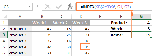
Instead of entering the row and column numbers in the formula, you can supply the cell references to get a more universal formula: =INDEX($B$2:$D$6, G2, G1)
So, this INDEX formula returns the number of items exactly at the intersection of the product number specified in G2 (row_num) and week number entered in cell G1 (column_num).
Tip. The use of absolute references ($B$2:$D$6) instead of relative references (B2:D6) in the array argument makes it easier to copy the formula to other cells. Alternatively, you can convert a range to a table ( Ctrl + T ) and refer to it by the table name.
INDEX array form — things to remember
- If the array argument consists of only one row or column, you may or may not specify the corresponding row_num or column_num argument.
- If the array argument includes more than one row and row_num is omitted or set to 0, the INDEX function returns an array of the entire column. Similarly, if array includes more than one column and the column_num argument is omitted or set to 0, the INDEX formula returns the entire row. Here’s a formula example that demonstrates this behavior.
- The row_num and column_num arguments must refer to a cell within array; otherwise, the INDEX formula will return the #REF! error.
INDEX reference form
The reference form of the Excel INDEX function returns the cell reference at the intersection of the specified row and column.
- reference — is one or several ranges.
If you are entering more than one range, separate the ranges by commas and enclose the reference argument in parentheses, for example (A1:B5, D1:F5).
If each range in reference contains only one row or column, the corresponding row_num or column_num argument is optional.
For example, the formula =INDEX((A2:D3, A5:D7), 3, 4, 2) returns the value of cell D7, which is at the intersection of the 3 rd row and 4 th column in the second area (A5:D7). 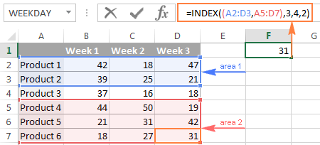
INDEX reference form — things to remember
- If the row_num or column_num argument is set to zero (0), an INDEX formula returns the reference for the entire column or row, respectively.
- If both row_num and column_num are omitted, the INDEX function returns the area specified in the area_num argument.
- All of the _num arguments (row_num, column_num and area_num) must refer to a cell within reference; otherwise, the INDEX formula will return the #REF! error.
Both of the INDEX formulas we’ve discussed so far are very simple and only illustrate the concept. Your real formulas are likely to be far more complex than that, so let’s explore a few most efficient uses of INDEX in Excel.
How to use INDEX function in Excel — formula examples
Perhaps there aren’t many practical uses of Excel INDEX by itself, but in combination with other functions such as MATCH or COUNTA, it can make very powerful formulas.
Source data
All of our INDEX formulas (except for the last one), we will use the below data. For convenience purposes, it is organized in a table named SourceData. 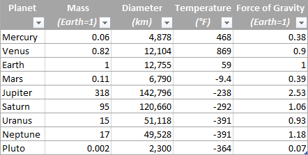
The use of tables or named ranges can make formulas a bit longer, but it also makes them significantly more flexible and better readable. To adjust any INDEX formula for your worksheets, you need only to modify a single name, and this fully makes up for a longer formula length.
Of course, nothing prevents you from using usual ranges if you want to. In this case, you simply replace the table name SourceData with the appropriate range reference.
1. Getting the N th item from the list
This is the basic use of the INDEX function and a simplest formula to make. To fetch a certain item from the list, you just write =INDEX(range, n) where range is a range of cells or a named range, and n is the position of the item you want to get.
When working with Excel tables, you can select the column using the mouse and Excel will pull the column’s name along with the table’s name in the formula: 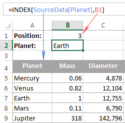 th item from the list» title=»An INDEX formula to get the N th item from the list» width=»251″ height=»246″>
To get a value of the cell at the intersection of a given row and column, you use the same approach with the only difference that you specify both — the row number and the column number. In fact, you already saw such a formula in action when we discussed INDEX array form.
And here’s one more example. In our sample table, to find the 2 nd biggest planet in the Solar system, you sort the table by the Diameter column, and use the following INDEX formula:
=INDEX(SourceData, 2, 3)
- Array is the table name, or a range reference, SourceData in this example.
- Row_num is 2 because you are looking for the second item in the list, which is in the 2 nd
- Column_num is 3 because Diameter is the 3 rd column in the table.
If you want to return the planet’s name rather than diameter, change column_num to 1. And naturally, you can use a cell reference in the row_num and/or column_num arguments to make your formula more versatile, as demonstrated in the screenshot below: 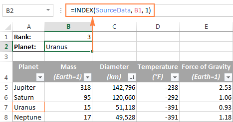
2. Getting all values in a row or column
Apart from retrieving a single cell, the INDEX function is able to return an array of values from the entire row or column. To get all values from a certain column, you have to omit the row_num argument or set it to 0. Likewise, to get the entire row, you pass empty value or 0 in column_num.
Such INDEX formulas can hardly be used on their own, because Excel is unable to fit the array of values returned by the formula in a single cell, and you would get the #VALUE! error instead. However, if you use INDEX in conjunction with other functions, such as SUM or AVERAGE, you will get awesome results.
For example, you could use the following formula to calculate the average planet temperature in the Solar system:
In the above formula, the column_num argument is 4 because Temperature in the 4 th column in our table. The row_num parameter is omitted. 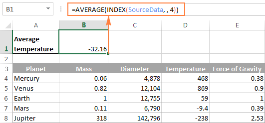
In a similar manner, you can find the minimum and maximum temperatures:
And calculate the total planet mass (Mass is the 2 nd column in the table):
From practical viewpoint, the INDEX function in the above formula is superfluous. You can simply write =AVERAGE(range) or =SUM(range) and get the same results.
When working with real data, this feature may prove helpful as part of more complex formulas you use for data analysis.
3. Using INDEX with other functions (SUM, AVERAGE, MAX, MIN)
From the previous examples, you might be under an impression that an INDEX formula returns values, but the reality is that it returns a reference to the cell containing the value. And this example demonstrates the true nature of the Excel INDEX function.
Since the result of an INDEX formula is a reference, we can use it within other functions to make a dynamic range. Sounds confusing? The following formula will make everything clear.
Suppose you have a formula =AVERAGE(A1:A10) that returns an average of the values in cells A1:A10. Instead of writing the range directly in the formula, you can replace either A1 or A10, or both, with INDEX functions, like this:
Both of the above formulas will deliver the same result because the INDEX function also returns a reference to cell A10 (row_num is set to 10, col_num omitted). The difference is that the range is the AVERAGE / INDEX formula is dynamic, and once you change the row_num argument in INDEX, the range processed by the AVERAGE function will change and the formula will return a different result.
Apparently, the INDEX formula’s route appears overly complicated, but it does have practical applications, as demonstrated in the following examples.
Example 1. Calculate average of the top N items in the list
Let’s say you want to know the average diameter of the N biggest planets in our system. So, you sort the table by Diameter column from largest to smallest, and use the following Average / Index formula:
=AVERAGE(C5 : INDEX(SourceData[Diameter], B1)) 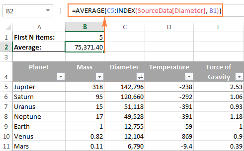
Example 2. Sum items between the specified two items
In case you want to define the upper-bound and lower-bound items in your formula, you just need to employ two INDEX functions to return the first and the last item you want.
For example, the following formula returns the sum of values in the Diameter column between the two items specified in cells B1 and B2:
=SUM(INDEX(SourceData[Diameter],B1) : INDEX(SourceData[Diameter], B2)) 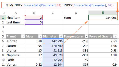
4. INDEX formula to create dynamic ranges and drop-down lists
As it often happens, when you start organizing data in a worksheet, you may not know how many entries you will eventually have. It’s not the case with our planets table, which seems to be complete, but who knows.
Anyway, if you have a changing number of items in a given column, say from A1 to An, you may want to create a dynamic named range that includes all cells with data. At that, you want the range to adjust automatically as you add new items or delete some of the existing ones. For example, if you currently have 10 items, your named range is A1:A10. If you add a new entry, the named range automatically expands to A1:A11, and if you change your mind and delete that newly added data, the range automatically reverts to A1:A10.
The main advantage of this approach is that you do not have to constantly update all formulas in your workbook to ensure they refer to correct ranges.
One way to define a dynamic range is using Excel OFFSET function:
=OFFSET(Sheet_Name!$A$1, 0, 0, COUNTA(Sheet_Name!$A:$A), 1)
Another possible solution is to use Excel INDEX together with COUNTA:
In both formulas, A1 is the cell containing the first item of the list and the dynamic range produced by both formulas will be identical.
The difference is in the approaches. While the OFFSET function moves from the starting point by a certain number of rows and/or columns, INDEX finds a cell at the intersection of a particular row and column. The COUNTA function, used in both formulas, gets the number of non-empty cells in the column of interest.
In this example, there are 9 non-blank cells in column A, so COUNTA returns 9. Consequently, INDEX returns $A$9, which is the last used cell in column A (usually INDEX returns a value, but in this formula, the reference operator (:) forces it to return a reference). And because $A$1 is our starting point, the final result of the formula is the range $A$1:$A$9.
The following screenshot demonstrates how you can use such Index formula to create a dynamic drop-down list. 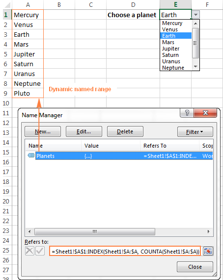
Tip. The easiest way to create an expandable dynamic data validation list is dropdown from a table. In this case, you won’t need any complex formulas since Excel tables are dynamic ranges per se.
You can also use the INDEX function to create dependent drop-down lists and the following tutorial explains the steps: Making a cascading drop-down list in Excel.
5. Powerful Vlookups with INDEX / MATCH
Performing vertical lookups — this is where the INDEX function truly shines. If you have ever tried using Excel VLOOKUP function, you are well aware of its numerous limitations, such as inability to pull values from columns to the left of the lookup column or 255 chars limit for a lookup value.
The INDEX / MATCH liaison is superior to VLOOKUP in many respects:
- No problems with left vlookups.
- No limit to the lookup value size.
- No sorting is required (VLOOKUP with approximate match does require sorting the lookup column in ascending order).
- You are free to insert and remove columns in a table without updating every associated formula.
- And the last but not the least, INDEX / MATCH does not slow down your Excel like multiple Vlookups do.
You use INDEX / MATCH in the following way:
For example, if we flip our source table so that Planet Name becomes the right-most column, the INDEX / MATCH formula still fetches a matching value from the left-hand column without a hitch. 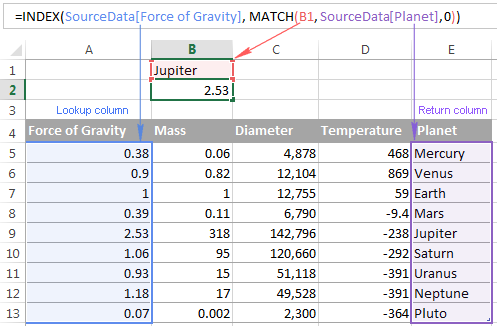
For more tips and formula example, please see the Excel INDEX / MATCH tutorial.
6. Excel INDEX formula to get 1 range from a list of ranges
Another smart and powerful use of the INDEX function in Excel is the ability to get one range from a list of ranges.
Suppose, you have several lists with a different number of items in each. Believe me or not, you can calculate the average or sum the values in any selected range with a single formula.
First off, you create a named range for each list; let it be PlanetsD and MoonsD in this example: 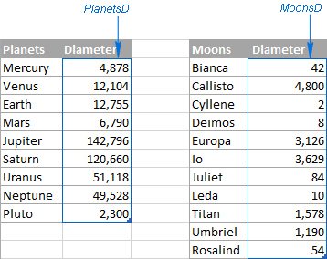
I hope the above image explains the reasoning behind the ranges’ names : ) BTW, the Moons table is far from complete, there are 176 known natural moons in our Solar System, Jupiter alone has 63 currently, and counting. For this example, I picked random 11, well. maybe not quite random — moons with the most beautiful names : )
Please excuse the digression, back to our INDEX formula. Assuming that PlanetsD is your range 1 and MoonsD is range 2, and cell B1 is where you put the range number, you can use the following Index formula to calculate the average of values in the selected named range:
=AVERAGE(INDEX((PlanetsD, MoonsD), , , B1))
Please pay attention that now we are using the Reference form of the INDEX function, and the number in the last argument (area_num) tells the formula which range to pick.
In the screenshot below, area_num (cell B1) is set to 2, so the formula calculates the average diameter of Moons because the range MoonsD comes 2 nd in the reference argument. 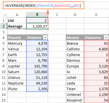
If you work with multiple lists and don’t want to bother remembering the associated numbers, you can employ a nested IF function to do this for you:
=AVERAGE(INDEX((PlanetsD, MoonsD), , , IF(B1=»planets», 1, IF(B1=»moons», 2))))
In the IF function, you use some simple and easy-to-remember list names that you want your users to type in cell B1 instead of numbers. Please keep this in mind, for the formula to work correctly, the text in B1 should be exactly the same (case-insensitive) as in the IF’s parameters, otherwise your Index formula will throw the #VALUE error.
To make the formula even more user-friendly, you can use Data Validation to create a drop-down list with predefined names to prevent spelling errors and misprints: 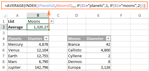
Finally, to make your INDEX formula absolutely perfect, you can enclose it in the IFERROR function that will prompt the user to choose an item from the drop-down list if no selection has been made yet:
=IFERROR(AVERAGE(INDEX((PlanetsD, MoonsD), , , IF(B1=»planet», 1, IF(B1=»moon», 2)))), «Please select the list!»)
This is how you use INDEX formulas in Excel. I am hopeful these examples showed you a way to harness the potential of the INDEX function in your worksheets. Thank you for reading!
Источник
We all deal with multiple sheets in a single workbook, don’t we? Here is a smart way to create an Index of all your Sheets. You can click on the sheet name to navigate to that sheet.
Here is how we do it
Assume that we have 5 Sheets
![]()
And we would like to have an Index placed (in a new sheet) with the sheet names hyperlinked to the respective sheet.
It can be done with a simple VBA Code
Here comes a Code
Sub CreateIndex()
Dim sheetnum As Integer
Sheets.Add before:=Sheets(1)
For sheetnum = 2 To Worksheets.Count
 ActiveSheet.Hyperlinks.Add _
 Anchor:=Cells(sheetnum - 1, 1), _
 Address:='', _
 SubAddress:=''' & Worksheets(sheetnum).Name & ''!A1', _
 TextToDisplay:=Worksheets(sheetnum).Name
Next sheetnum
ActiveWindow.DisplayGridlines = False
End Sub
Follow the steps
- Copy this Code
- Open the excel workbook where you want to create a Sheet Index
- Press the shortcut Alt + F11 to open the Visual Basic Window
- In the Insert Menu, click on Module or use the shortcut Alt i m to add a Module. Module is the place where the code is written
- In the blank module paste the code and close the Visual Basic Editor
- Then use the shortcut Alt + F8 to open the Macro Box. You would have the list of all the macros here
- You would see the Macro that you have just pasted in the Module as ‘CreateIndex’
- Run it. You would see an Index with all the sheet names hyperlinked to the respective sheet.
Other Useful Macros
- Automated Filter with Macro
- Unhiding Multiple Sheets at Once
- Covert Numbers into Indian Currency Words
Topics that I write about…

goodly
In this post we’ll find out how to get a list of all the sheet names in the current workbook without using VBA.
This can be pretty handy if you have a large workbook with hundreds of sheets and you want to create a table of contents. This method uses the little known and often forgotten Excel 4 macro functions.
These functions aren’t like Excel’s other functions such as SUM, VLOOKUP, INDEX etc. These functions won’t work in a regular sheet, they only work in named functions and macro sheets. For this trick we’re going to use one of these in a named function.
In this example, I’ve created a workbook with a lot of sheets. There are 50 sheets in this example so I was lazy and didn’t rename them from the default names.
Now we will create our named function.
- Go to the Formulas tab.
- Press the Define Name button.
- Enter SheetNames into the name field.
- Enter the following formula into the Refers to field.
=REPLACE(GET.WORKBOOK(1),1,FIND("]",GET.WORKBOOK(1)),"") - Hit the OK button.
In a sheet within the workbook enter the numbers 1,2,3,etc… into column A starting at row 2 and then in cell B2 enter the following formula and copy and paste it down the column until you have a list of all your sheet names.
=INDEX(SheetNames,A2)As a bonus, we can also create a hyperlink so that if you click on the link it will take you to that sheet. This can be handy for navigating through a spreadsheet with lots of sheets. To do this add this formula into the column C.
= HYPERLINK ( "#'" & B2 & "'!A1", "Go To Sheet" )Note, to use this method you will need to save the file as a macro enabled workbook (.xls, .xlsm or .xlsb). Not too difficult and no VBA needed.
Video Tutorial
This video will show you two methods to list all the sheet names in a workbook.
- The first method uses a VBA procedure from this post.
- The second (skip to 3:15 in the video) uses the method in the above post.
About the Author
John is a Microsoft MVP and qualified actuary with over 15 years of experience. He has worked in a variety of industries, including insurance, ad tech, and most recently Power Platform consulting. He is a keen problem solver and has a passion for using technology to make businesses more efficient.
![]()
Download Article
![]()
Download Article
If your Excel workbook contains numerous worksheets, you can add a table of contents that indexes all of your sheets with clickable hyperlinks. This tutorial will teach you how to make an index of sheet names with page numbers in your Excel workbook without complicated VBA scripting, and how to add helpful «back to index» buttons to each sheet to improve navigation.
-

1
Create an index sheet in your workbook. This sheet can be anywhere in your workbook, but you’ll usually want to place the tab at the beginning like a traditional table of contents.
- To create a new sheet, click the + at the bottom of the active worksheet. Then, right-click the new tab, select Rename, and type a name for your sheet like Index or Worksheets.
- You can rearrange sheets by dragging their tabs left or right at the bottom of your workbook.
-
2
Type Page Number into cell A1 of your index sheet. Column A is where you’ll be placing the page numbers for each sheet.
Advertisement
-
3
Type Sheet Name into cell B1 of your index sheet. This will be the column header above your list of worksheets.
-
4
Type Link into cell C1 of your index sheet. This is the column header that will appear above hyperlinks to each worksheet.
-
5
Click the Formulas tab. It’s at the top of Excel.
-
6
Click Define Name. It’s on the «Defined Names» tab at the top of Excel.
-
7
Type SheetList into the «Name» field. This names the formula you’ll be using with the INDEX function.[1]
-
8
Type the formula into the «Refers to» field and click OK. The formula is =REPLACE(GET.WORKBOOK(1),1,FIND("]",GET.WORKBOOK(1)),"").
-
9
Enter page numbers in column A. This is the only part you’ll have to do manually. For example, if your workbook has 20 pages, you’ll type 1 into A2, 2 into A3, etc., and continue numbering down until you’ve entered all 20 page numbers.
- To quickly populate the page numbers, type the first two page numbers into A2 and A3, click A3 to select it, and then drag the square at A3’s bottom-right corner down until you’ve reached the number of pages in your workbook. Then, click the small icon with a + that appears at the bottom-right corner of the column and select Fill Series.
-
10
Type this formula into cell B2 of your index sheet. The formula is =INDEX(SheetList,A2). When you press Enter or Return, you’ll see the name of the first sheet in your workbook.
-
11
Fill the rest of column B with the formula. To do this, just click B2 to select it, and then double-click the square at its bottom-right corner. This adds the name of each worksheet corresponding to the page numbers you typed into column A.
-
12
Type this formula into C2 of your worksheet. The formula is =HYPERLINK("#'"&B2&"'!A1","Go to Sheet"). When you press Enter or Return, you’ll see a hyperlink to the first page in your index called «Go to Sheet.»
-
13
Fill the rest of column C with the formula. To do this, click C2 to select it, and then double-click the square at its bottom-right corner. Now each sheet in your workbook has a clickable hyperlink that takes you right to that page.
-
14
Save your workbook in the macro-enabled format. Because you created a named range, you’ll need to save your workbook in this format.[2]
Here’s how:- Go to File > Save.
- On the pop-up message that warns you about saving a macro-free workbook, click No.
- In the «Save as type» or file format menu, select Excel Macro-Enabled Workbook (*.xlsm) and click Save.


Advertisement
-
1
Click your index or table of contents sheet. If you have a lot of pages in your workbook, it’ll be helpful to readers to add quick «Back to Index» or «Back to Table of Contents» links to each sheet so they don’t have to scroll through lots of worksheet tabs after clicking to that page. Start by opening your index sheet.
-
2
Name the index. To do this, just click the field directly above cell A1, type Index, and then press Enter or Return.
- Don’t worry if the field already contains a cell address.
-
3
Click any of the sheets in your workbook. Now you’ll create your back button. Once you create a back button on one sheet, you can just copy and paste it onto other sheets.
-
4
Click the Insert tab. It’s at the top of the screen.
-
5
Click the Illustrations menu and select Shapes. This option will be in the upper-left area of Excel.
-
6
Click a shape for your button. For example, if you want to create a back-arrow icon sort of like your web browser’s back button, you can click the left-pointing arrow under the «Block Arrows» header.
-
7
Click the location where you want to place the button. Once you click, the shape will appear. If you want, you can change the color and look using the options at the top, and/or resize the shape by dragging any of its corners.
-
8
Type some text onto the shape. The text you type should be something like «Back to Index.» You can double-click the shape to place the cursor and start typing right onto the actual shape
- You might need to drag the corner of the shape to resize it so the text fits.
- To place a text box on or near the shape before typing, just click the Shape Format menu at the top (while the shape is selected), click Text Box in the toolbar, and then click and drag a text box.
- You can stylize the text using the options in Text on the toolbar while the shape is selected.
-
9
Right-click the shape and select Link. This opens the Insert Hyperlink dialog.[3]
-
10
Click the Place in This Document icon. It’s in the left panel.
-
11
Select your index under «Defined Names» and click OK. You might have to click the + next to the column header to see the Index option. This makes the text in the shape a clickable hyperlink that takes you right to the index.
-
12
Copy and paste the hyperlink to other sheets. To do this, just right-click the shape and select Copy. Then, you can paste it onto any other page by right-clicking the desired location and selecting the first icon under «Paste Options» (the one that says «Use Destination Theme» when you hover the mouse over it).


Advertisement
Ask a Question
200 characters left
Include your email address to get a message when this question is answered.
Submit
Advertisement
Thanks for submitting a tip for review!
About This Article
Article SummaryX
To create a table of contents in Excel, you can use the «Defined Name» option to create a formula that indexes all sheet names on a single page. Then, you can use the INDEX function to list the sheet names, as well as the HYPERLINK function to create quick links to each sheet.
Did this summary help you?
Thanks to all authors for creating a page that has been read 55,649 times.
Is this article up to date?
In the ongoing project of mine, with which I’m about to be done, I want to make sure that the people taking over my job will be left with something that won’t break after I’m gone. This project is an ongoing tracker kept daily throughout the year and each worksheet used (several for varying items of interest) are separated out by year in the name of the worksheet. For instance, the primary sheet is simply called ‘YYYY’ in which the ‘YYYY’ is the current year. Other worksheets are called, ‘DTDYYYY’, ‘MTDYYYY’, ‘YTDYYYY’ in which the YYYY is the current year. Come 2013, I’d like it if the little VBA that I use is able to take the current YYYY and find the appropriate worksheets automagically.
I know that I can reference sheets using the SheetIDX convention. I know that I can use Sheets(NAME) method. I’m not so sure how to best go about accomplishing my goal, though.
![]()
asked Jan 7, 2012 at 5:45
![]()
2
Application.Sheets("Sheet1").Index
Application.Sheets(1).Name
Hope this is what you needed.
Sorry, I didn’t see the last part about current year. Perhaps this?
Application.Sheets(Year(Date())).Activate
answered Jan 7, 2012 at 6:03
![]()
TimTim
1,0116 silver badges12 bronze badges
1
You need a string for the name.
With ThisWorkbook
    .Sheets(CStr(Year(Date))).Select
End With
answered Jan 7, 2012 at 19:48
![]()
FionnualaFionnuala
90.1k7 gold badges110 silver badges148 bronze badges
|
Limos Пользователь Сообщений: 102 |
#1 05.07.2017 14:56:55 Добрый день! Подскажите как правильно получить следующую информацию.
Звездочка означает, что неважно какие символы будут дальше. Заранее спасибо. |
||
|
vikttur Пользователь Сообщений: 47199 |
В цикле проверяйте наличие фрагмента в имени листа. |
|
Limos Пользователь Сообщений: 102 |
Каким образом, подскажите приблизительно. |
|
_Boroda_  Пользователь Сообщений: 1496 Контакты см. в профиле |
#4 05.07.2017 15:15:03 Приблизительно так
Изменено: _Boroda_ — 05.07.2017 15:15:11 Скажи мне, кудесник, любимец ба’гов… |
||
|
vikttur Пользователь Сообщений: 47199 |
#5 05.07.2017 15:17:45
|
||
|
Limos Пользователь Сообщений: 102 |
#6 05.07.2017 15:34:42 Спасибо большое) Я это находил чтобы обновить источник данных для сводной таблицы, вот код
Но, гад выдает ошибку Run-time error ’91’ Object variable or With block variable not set Изменено: Limos — 05.07.2017 15:46:01 |
||
When working with Excel spreadsheets, sometimes you may have a need to get the name of the worksheet.
While you can always manually enter the sheet name, it won’t update in case the sheet name is changed.
So if you want to get the sheet name, so that it automatically updates when the name is changed, you can use a simple formula in Excel.
In this tutorial, I will show you how to get the sheet name in Excel using a simple formula.
Get Sheet Name Using the CELL Function
CELL function in Excel allows you to quickly get information about the cell in which the function is used.
This function also allows us to get the entire file name as a result of the formula.
Suppose I have an Excel workbook with the sheet name ‘Sales Data’
Below is the formula that I have used in any cells in the ‘Sales Data’ worksheet:
=CELL("filename"))
As you can see, it gave me the whole address of the file in which I am using this formula.
But I needed only the sheet name, not the whole file address,
Well, to get the sheet name only, we will have to use this formula along with some other text formulas, so that it can extract only the sheet name.
Below is the formula that will give you only the sheet name when you use it in any cell in that sheet:
=RIGHT(CELL("filename"),LEN(CELL("filename"))-FIND("]",CELL("filename")))
The above formula will give us the sheet name in all scenarios. And the best part is that it would automatically update in case you change the sheet name or the file name.
Note that the CELL formula only works if you have saved the workbook. If you haven’t, then it would return a blank (as it has no idea what the workbook path is)
Wondering how this formula works? Let me explain!
The CELL formula gives us the whole workbook address along with the sheet name at the end.
One rule it would always follow is to have the sheet name after the square bracket (]).
Knowing this, we can find out the position of the square bracket, and then extract everything after it (which would be the sheet name)
And that’s exactly what this formula does.
The FIND part of the formula looks for ‘]’ and return it’s position (which is a number that denotes the number of characters after which the square bracket is found)
We use this position of the square bracket within the RIGHT formula to extract everything after that square bracket
One major issue with the CELL formula is that it’s dynamic. So if you use it in Sheet1 and then go to Sheet2, the formula in Sheet1 would update and show you the name as Sheet2 (despite the formula being on Sheet1). This happens as the CELL formula considers the cell in the active sheet and gives the name for that sheet, no matter where it is in the workbook. A workaround would be to hit the F9 key when you want to update the CELL formula in the active sheet. This will force a recalculation.
Alternative Formula to Get Sheet Name (MID formula)
There are many different ways to do the same thing in Excel. And in this case, there is another formula that works just as well.
Instead of the RIGHT function, it uses the MID function.
Below is the formula:
=MID(CELL("filename"),FIND("]",CELL("filename"))+1,255)
This formula works similarly to the RIGHT formula, where it first finds the position of the square bracket (using the FIND function).
It then uses the MID function to extract everything after the square bracket.
Fetching Sheet Name and Adding Text to it
If you’re building a dashboard, you may want to not just get the name of the worksheet, but also append a text before or after it.
For example, if you have a sheet name 2021, you may want to get the result as ‘Summary of 2021’ (and not just the sheet name).
This can easily be done by combining the formula we saw above with the text we want before it using the ampersand operator.
Below is the formula that will add the text ‘Summary of ‘ before the sheet name:
="Summary of "&RIGHT(CELL("filename"),LEN(CELL("filename"))-FIND("]",CELL("filename")))
The ampersand operator (&) simply combines the text before the formula with the result of the formula. You can also use the CONCAT or CONCATENATE function instead of an ampersand.
Similarly, if you want to add any text after the formula, you can use the same ampersand logic (i.e., have the ampersand after the formula followed by the text that you want to append).
So these are two simple formulas that you can use to get the sheet name in Excel.
I hope you found this tutorial useful.
Other Excel tutorials you may also like:
- How to Rename a Sheet in Excel (4 Easy Ways + Shortcut)
- How to Insert New Worksheet in Excel (Easy Shortcuts)
- How to Unhide Sheets in Excel (All In One Go)
- How to Sort Worksheets in Excel using VBA (alphabetically)
- Combine Data From Multiple Worksheets into a Single Worksheet in Excel
- How to Compare Two Excel Sheets
- How to Group Worksheets in Excel
Return to Excel Formulas List
Download Example Workbook
Download the example workbook
This tutorial demonstrates how to list the sheet names of a workbook with a formula in Excel.
List Sheet Names Using Named Range and Formula
There is no built-in function in Excel that can list all the worksheets in a workbook. Instead you have two options:
- Use a VBA Macro to list all sheets in the workbook
- Create a Formula to list all sheets
If you want to use a formula, follow these steps:
- Create a named range “Worksheets”
- Use a formula to list out all sheet names.
Create Name Range for Sheet Names
To create a Named Range for the sheet names, in the Excel Ribbon: Formulas > Name Manager > New
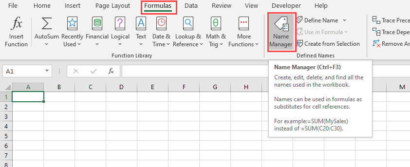
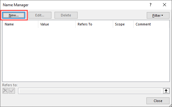
Type “Worksheets” in the Name Box:
In the “Refers to” section of the dialog box, we will need to write the formula
=GET.WORKBOOK(1) & T(NOW())"This formula stores the names of all sheets (as an array in this format: “[workbook.xlsm].Overview”) in the workbook to the named range “Worksheets”.
The “GET.WORKBOOK” Function is a macro function, so your workbook has to be saved as a macro-enabled workbook (file format: .xlsm) for the sheet names to be updated each time the workbook is opened.
Note: When filling the Edit name dialog box, workbook should be selected as the scope of the name range.
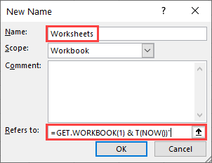
Using Formula to List Sheet Names
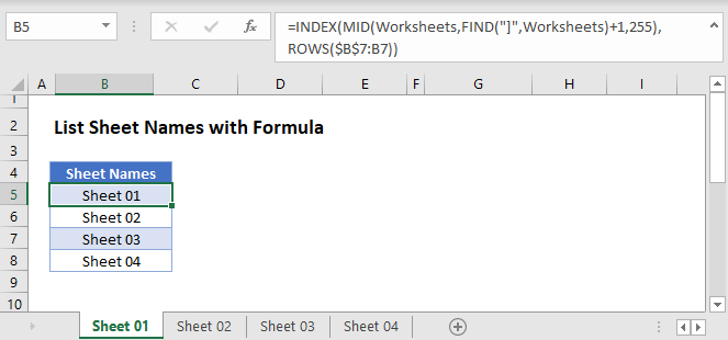
Now we use a formula to list the sheet names. We’ll need the INDEX, MID, FIND, and ROWS Functions:
=INDEX(MID(Worksheets,FIND("]",Worksheets)+1,255),ROWS($B$5:B5))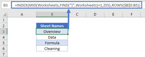
- The formula above takes the “Worksheets” array and displays each sheet name based on its position.
- The MID and FIND Functions extract the sheet names from the array (removing the workbook name).
- Then the INDEX and ROW Functions display each value in that array.
- Here, “Overview” is the first sheet in the workbooks and “Cleaning” is the last.
Click the link for more information on how the MID and FIND Functions get sheet names.
Alternate Method
You also have the option to create the list of sheet names within the Name Manager. Instead of
=GET.WORKBOOK(1) & T(NOW())set your “Refers to” field to
=REPLACE(GET.WORKBOOK(1),1,FIND("]",GET.WORKBOOK(1)),"")Now there’s no need for MID, FIND, and ROWS in your formula. Your named range is already made up of only sheet names.
Use this simpler INDEX formula to list the sheets:
=INDEX(SheetName,B3)
Navigating workbooks with lots of sheets can be tedious. In this tutorial I’m going to show you how to dynamically list Excel sheet names and add some user-friendly hyperlinks to help users easily navigate the file.
It requires an old Excel 4.0 Macro Function called GET.WORKBOOK and this means the file must be saved as a .xlsm file type. Don’t let that put you off though. It’s super easy and doesn’t require any macro/VBA programming knowledge.
Watch the Video

Download Workbook
Enter your email address below to download the sample workbook.
By submitting your email address you agree that we can email you our Excel newsletter.
The crux of this solution is the GET.WORKBOOK function which returns information about the Excel file. The syntax is:
=GET.WORKBOOK(type_num, name_text)
type_num refers to various properties in the workbook. Type_num 1 returns the list of sheet names and that’s what we’ll be using.
name_text is the name of the workbook you want to get the sheet names from. We’re going to omit this argument, and it will simply return the names from the active workbook.
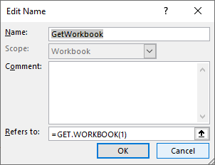
Excel 4.0 macro functions like GET.WORKBOOK cannot be typed in cells like the functions we know and love today, they must be defined in a name.
I’ve defined a name (Formulas tab > Define Name) GetWorkbook as you can see below:
And if I reference that name in a formula it returns the list of sheet names prefixed by the file name.
You can see in the image below that I wrapped the defined name in the TRANSPOSE function because GET.WORKBOOK returns a horizontal array of sheet names and I wanted them in a vertical array.
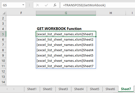
Note: I have Excel for Microsoft 365 with dynamic arrays, so my formula spills the results to the cells below, as denoted by the blue border around cells B6:B12 in the image above.
If you have Excel 2019 or earlier you need a different formula, but more on that later. First, I just want to explain what GET.WORKBOOK does.
Now, I only want the sheet names, so I’ll use the REPLACE function with FIND to extract them:
=REPLACE(GET.WORKBOOK(1),1,FIND("]",GET.WORKBOOK(1)),"")
Tip: you could use the SUBSTITUTE function instead of REPLACE.
Lastly, to ensure the formula dynamically updates I’m going to append the volatile function, NOW, wrapped in the T function on the end:
=REPLACE(GET.WORKBOOK(1),1,FIND("]",GET.WORKBOOK(1)),"")&T(NOW())
We do this because NOW, which returns the current time, triggers a recalculation of the defined name. The T function returns blank when the value returned isn’t text. In other words, T hides the time returned by NOW. The only reason we’re appending the NOW function is because it’s a volatile function that triggers a recalculation of the defined name which is required to update the list of sheet names.
I’ll define a new name for this formula, SheetNames:
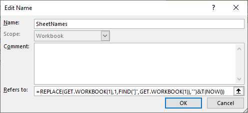
And when you enter this formula wrapped in TRANSPOSE in a cell it returns the sheet names:
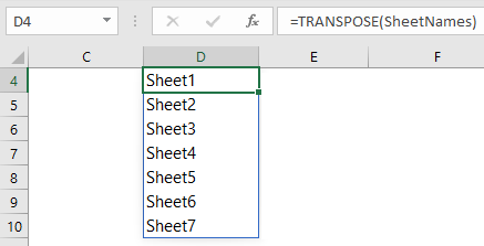
Again, my formula spills the results to the cells below because I have dynamic arrays.
Dynamically List Excel Sheet Names — Excel 2019 and Earlier
In all versions of Excel we can use the INDEX function with ROW to return the list of sheet names:
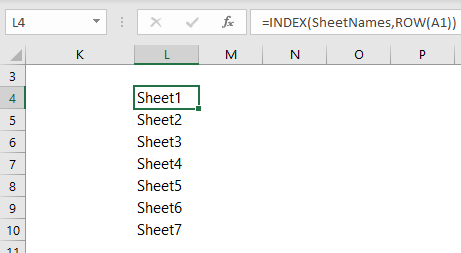
Note: the ROW function simply returns the row number of a cell. The ROW function in the formula in the image above returns 1. As you copy it down the column it returns 2, then 3 and so on. However, if you copy the formula down more rows than you have sheets for it will return an error.
We can handle the errors with the IFERROR function:
=IFERROR(INDEX(SheetNames,ROW(A1)),"")
This allows you to copy it down past the current number of sheets you have which will ensure any new sheets added are automatically included in the list.
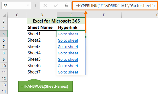
Dynamically List Excel Sheet Names with Hyperlinks
Of course, what good is a list of Excel sheet names without hyperlinks to take you to those sheets? To solve this we can nest the INDEX formula inside HYPERLINK:
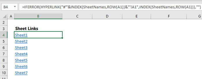
=IFERROR(HYPERLINK("#'"&INDEX(SheetNames, ROW(A1))&"'!A1", INDEX(SheetNames,ROW(A1))),"")
Copy the formula down to get a list of sheet names with ready-made hyperlinks:
Be sure to copy the formula down past the last current sheet name so that new sheets are automatically included.
More on the HYPERLINK function here.
Note: you may find that the formula doesn’t automatically update. If that happens, press F9 to force a recalculation, or perform any of the other actions that trigger recalculations.
Excel for Microsoft 365
If you have dynamic arrays you might be wondering if this can be done using spilled ranges and the answer is kind of. It requires the sheet name and hyperlink to be in separate columns, as you can see below:
The formula in column D spills the results and will grow as new sheets are added. The formula in column E references the spilled range with D5# and will therefore also grow as new sheets are added. Unfortunately, you cannot create a single formula by replacing D5# in column E’s formula with ‘SheetNames’ or ‘TRANSPOSE(SheetNames)’.
Limitations
This technique has a few limitations:
- It includes hidden sheets however the hyperlink can’t open a hidden sheet
- It requires the file to be saved as a .xlsm and macros enabled
- Requires recalculation to add new sheets to the list. The T(NOW()) part of the formula will trigger recalculation based on various actions, but if you don’t perform any of those actions, you can force a recalculation by pressing the F9 key.
Related Lessons
We can also generate a list if Excel Sheet Names with VBA
And you can get a complete list of the elusive Excel 4.0 Macro Functions here.