
Is there a harder working team in Excel, than the reliable duo of INDEX and MATCH? These functions work beautifully together, with MATCH identifying the location of an item, and INDEX pulling the results out from the murky depths of data. See how to find text with INDEX and MATCH.
Find Text in a String
Last week, Jodie asked if I could help with a problem, and INDEX and MATCH came to the rescue again.
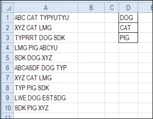
Jodie sent me a picture of her worksheet, with text strings in column A and codes in column D. Each text string contained one of the codes, and Jodie wanted that code to appear in column B.
Would you use INDEX and MATCH to find the code, or another method? Keep reading to see my solution, and please share your ideas, if you have other ways to solve this.

Count the Occurrences With COUNTIF
When you want to find text that’s buried somewhere in a string, the * wildcard character is useful. We can use the wildcard with COUNTIF, to see if the string is found somewhere in the text.
I entered this test formula in cell B1. This formula needs to be array-entered, so press Ctrl + Shift + Enter.
=COUNTIF(A1,”*” & $D$1:$D$3 & “*”)

There are wildcard characters before and after the cell references to D1:D3, so the text will be found anywhere within the text string.
To see the results of the array formula, click in the formula bar, and press the F9 key. The array shows 0;1;0 so it found a match for CAT, which is in the second cell in the range, $D$1:$D$3.
- Important: After you check the results, press the Esc key, to exit the formula without saving the calculated results.

Get the Position With MATCH
Next, you can add the MATCH function, wrapped around the COUNTIF formula, to get the position of the “1” in the results.
Make the following change to the formula in cell B1, and remember to press Ctrl + Shift + Enter.
=MATCH(1,COUNTIF(A1,”*”&$D$1:$D$3&”*”),0)

The result is 2, so the code “CAT”, the 2nd item in range D1:D3, was found in cell A1.
Get the Code With INDEX
Next, the INDEX function can return the code from the range $D$1:$D$3, that is at the position that the MATCH function identified.
Make the following change to the formula in cell B1, and remember to press Ctrl + Shift + Enter.
=INDEX($D$1:$D$3,MATCH(1,COUNTIF(A1,”*”&$D$1:$D$3&”*”),0))

The result is CAT, so the formula is working correctly.
Prevent Error Results With IFERROR
There should be one valid code in each text string, but sometimes the data doesn’t cooperate. Just in case there are text strings without a code, or more than one instance of the code, you can use IFERROR to show an empty string, instead of an error. (Excel 2007 and later versions)
=IFERROR(INDEX($D$1:$D$3,MATCH(1,COUNTIF(A1,”*”&$D$1:$D$3&”*”),0)),””)
Enter with Ctrl + Shift + Enter, and then copy the formula down to row 10.

In cell B6, the formula returns an empty string, and the cell looks blank, because none of the valid codes are in the text that’s in cell A6.
Use a Named Range
Instead of referring to range $D$1:$D$3, you could name that range, and use the name in the INDEX/MATCH formula. That would make it easier to maintain, if the size of the codes list will change.

Download Find Text With INDEX and MATCH Sample File
To get the sample file, and see how the formula works, go to the INDEX and MATCH page on my Contextures site.
In the Download section on that page, look for sample file 4 – Find Text From Code List. The zipped file is in xlsx format, and does not contain macros.
More INDEX and MATCH Examples
There are more examples of using INDEX and MATCH on my Contextures site.
____________________________
In Excel, there are multiple string (text) functions that can help you to deal with textual data. These functions can help you to change a text, change the case, find a string, count the length of the string, etc. In this post, we have covered top text functions. (Sample Files)
1. LEN Function
LEN function returns the count of characters in the value. In simple words, with the LEN function, you can count how many characters are there in value. You can refer to a cell or insert the value in the function directly.
Syntax
LEN(text)
Arguments
- text: A string for which you want to count the characters.
Example
In the below example, we have used the LEN to count letters in a cell. “Hello, World” has 10 characters with a space between and we have got 11 in the result.

In the below example, “22-Jan-2016” has 11 characters, but LEN returns 5.

The reason behind it is that the LEN function counts the characters in the value of a cell and is not concerned with formatting.
Related: How to COUNT Words in Excel
2. FIND Function
FIND function returns a number which is the starting position of a substring in a string. In simple words, by using the find function you can find (case sensitive) a string’s starting position from another string.
Syntax
FIND(find_text,within_text,[start_num])
Arguments
- find_text: The text which you want to find from another text.
- within_text: The text from which you want to locate the text.
- [start_num]: The number represents the starting position of the search.
Example
In the below example, we have used the FIND to locate the “:” and then with the help of MID and LEN, we have extracted the name from the cell.
3. SEARCH Function
SEARCH function returns a number which is the starting position of a substring in a string. In simple words, with the SEARCH function, you can search (non-case sensitive) for a text string’s starting position from another string.
Syntax
SEARCH(find_text,within_text,[start_num])
Arguments
- find_text: A text which you want to find from another text.
- within_text: A text from which you want to locate the text. You can refer to a cell, or you can input a text in your function.
Example
In the below example, we are searching for the alphabet “P” and we have specified start_num as 1 to start our search. Our formula returns 1 as the position of the text.

But, if you look at the word, we also have a “P” in the 6th position. That means the SEARCH function can only return the position of the first occurrence of a text, or if you specify the start position accordingly.
4. LEFT Function
LEFT Functions return sequential characters from a string starting from the left side (starting). In simple words, with the LEFT function, you can extract characters from a string from its left side.
Syntax
LEFT(text,num_chars)
Arguments
- text: A text or number from which you want to extract characters.
- [num_char]: The number of characters you want to extract.
Example
In the below example, we have extracted the first five digits from a text string using LEFT by specifying the number of characters to extract.

In the below example, we have used LEN and FIND along with the LEFT to create a formula that extracts the name from the cell.

5. RIGHT Function
The RIGHT function returns sequential characters from a string starting from the right side (ending). In simple words, with the RIGHT function, you can extract characters from a string from its left side.
Syntax
RIGHT(text,num_chars)
Arguments
- text: A text or number from which you want to extract characters.
- [num_char]: A number of characters you want to extract.
Example
In the below example, we have extracted 6 characters using the right function. If you know, how many characters you need to extract from the string, you can simply extract them by using a number.

Now, if you look at the below example, where we have to extract the last name from the cell, but we are not confirmed about the number of characters in the last name.

So, we are using LEN and FIND to get the name. Let me show you how we have done this.
First of all, we have used the LEN to get the length of that entire text string, then we used the FIND to get the position number of space between first and last names. And in the end, we have used both the figures to get the last name.
Arguments
- value1: A cell reference, an array, or a number that is directly entered into the function.
- [value2]: A cell reference, an array, or a number that is directly entered into the function.
6. MID Function
MID returns a substring from a string using a specific position and number of characters. In simple words, with MID, you can extract a substring from a string by specifying the starting character and number of characters you want to extract.
Syntax
MID(text,start_num,num_chars)
Arguments
- text: A text or a number from which you want to extract characters.
- start_char: A number for the position of the character from where you want to extract characters.
- num_chars: The number of characters you want to extract from the start_char.
Example
In the below example, we have used different values:
- From the 6th character to the next 6 characters.
- From the 6th character to the next 10 characters.
- We have used starting a character in negative and it has returned an error.
- By using 0 for the number of characters to extract and it has returned a blank.
- With a negative number for the number of characters to extract and it has returned an error.
- The starting number is zero and it has returned an error.
- Text string directly into the function.

7. LOWER Function
LOWER returns the string after converting all the letters in small. In simple words, it converts a text string where all the letters you have are in small letters, numbers will stay intact.
Syntax
LOWER(text)
Arguments
- text: The text which you want to convert to the lowercase.
Example
In the below example, we have compared the lower case, upper case, proper case, and sentence case with each other.

A lower case text has all the letters in a small case compared to others.
8. PROPER Function
The PROPER function returns the text string into a proper case. In simple words, with a PROPER function where the first letter of the word is in capital and rest in small (proper case).
Syntax
PROPER(text)
Arguments
- text: The text which you want to convert to the proper case.
Example
In the below example, we have a proper case that has the first letter in the capital case in a word and the rest of the letters are in the lower case compared to the other two cases lowercase and uppercase.

In the below example, we have used the PROPER function to streamline first name and last name into the proper case.

9. UPPER Function
The UPPER function returns the string after converting all the letters in the capital. In simple words, it converts a text string where all the letters you have are in capital form and numbers will stay intact.
Syntax
UPPER(text)
Arguments
- text: The text which you want to convert into uppercase.
Example
In the below example, we have used the UPPER to convert name text to capital letters from the text in which characters are in different cases.

10. REPT Function
REPT function returns a text value several times. In simple words, with the REPT function, you can specify a text, and a number to repeat that text.
Syntax
REPT(value1, [value2], …)
Example
In the below example, we have used different type of text for repetition using REPT. It can repeat any type of text or numbers and even symbols that you specify in function and the main use of the REPT function is for creating in-cell charts.

-
— By
Sumit Bansal
In this tutorial, you’ll learn how to find the position of the last occurrence of a character in a string in Excel.
A few days ago, a colleague came up with this problem.
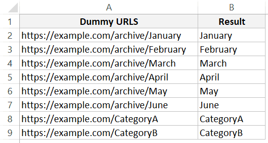
He had a list of URLs as shown below, and he needed to extract all the characters after the last forward slash (“/”).
So for example, from https://example.com/archive/January he had to extract ‘January’.
It would have been really easy has there been only one forward slash in the URLs.
What he had was a huge list of thousands on URLs of varying length and a varying number of forward-slashes.
In such cases, the trick is to find the position of the last occurrence of the forward slash in the URL.
In this tutorial, I will show you two ways to do this:
- Using an Excel formula
- Using a custom function (created via VBA)
Getting the Last Position of a Character using Excel Formula
When you have the position of the last occurrence, you can simply extract anything on the right of it using the RIGHT function.
Here is the formula that would find the last position of a forward slash and extract all the text to the right of it.
=RIGHT(A2,LEN(A2)-FIND("@",SUBSTITUTE(A2,"/","@",LEN(A2)-LEN(SUBSTITUTE(A2,"/",""))),1))

How does this formula work?
Let ‘s break down the formula and explain how each part of it works.
- SUBSTITUTE(A2,”/”,“”) – This part of the formula replaces the forward slash with an empty string. So for example, In case you want to find the occurrence of any string other than the forward slash, use that here.
- LEN(A2)-LEN(SUBSTITUTE(A2,”/”,“”)) – This part would tell you how many forward slashes are there in the string. It simply subtracts the length of the string without the forward slash from the length of the string with forward-slashes.
- SUBSTITUTE(A2,”/”,”@”,LEN(A2)-LEN(SUBSTITUTE(A2,”/”,””))) – This part of the formula would replace the last forward slash with @. The idea is to make that character unique. You can use any character you want. Just make sure it’s unique and doesn’t appear in the string already.
- FIND(“@”,SUBSTITUTE(A2,”/”,”@”,LEN(A2)-LEN(SUBSTITUTE(A2,”/”,””))),1) – This part of the formula would give you the position of the last forward slash.
- LEN(A2)-FIND(“@”,SUBSTITUTE(A2,”/”,”@”,LEN(A2)-LEN(SUBSTITUTE(A2,”/”,””))),1) – This part of the formula would tell us how many characters are there after the last forward slash.
- =RIGHT(A2,LEN(A2)-FIND(“@”,SUBSTITUTE(A2,”/”,”@”,LEN(A2)-LEN(SUBSTITUTE(A2,”/”,””))),1)) – Now this would simply give us the string after the last forward slash.
Getting the Last Position of a Character using Custom Function (VBA)
While the above formula is great and works like a charm, it’s a bit complicated.
If you’re comfortable using VBA, you can use a custom function (also called a User Defined Function) created via VBA. This can simplify the formula and can save time if you have to do this often.
Let’s use the same data set of URLs (as shown below):
For this case, I have created a function called LastPosition, that find the last position of the specified character (which is a forward slash in this case).
Here is the formula that will do this:
=RIGHT(A2,LEN(A2)-LastPosition(A2,"/")+1)

You can see that this is a lot simpler than the one we used above.
Here is how this works:
- LastPosition – which is our custom function – returns the position of the forward-slash. This function takes two arguments – the cell reference that has the URL and the character whose position we need to find.
- RIGHT function then gives us all the characters after the forward slash.
Here is the VBA code that created this function:
Function LastPosition(rCell As Range, rChar As String)
'This function gives the last position of the specified character
'This code has been developed by Sumit Bansal (https://trumpexcel.com)
Dim rLen As Integer
rLen = Len(rCell)
For i = rLen To 1 Step -1
If Mid(rCell, i - 1, 1) = rChar Then
 LastPosition = i
 Exit Function
End If
Next i
End Function
To make this function work, you need to place it in the VB Editor. Once done, you can use this function like any other regular Excel function.
Here are the steps to copy and paste this code in the VB back-end:
Here are the steps to place this code in the VB Editor:
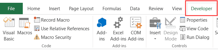
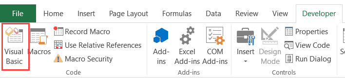
- Go to the Developer tab.

- Click on the Visual Basic option. This will open the VB editor in the backend.
- In the Project Explorer pane in the VB Editor, right-click on any object for the workbook in which you want to insert the code. If you don’t see the Project Explorer go to the View tab and click on Project Explorer.
- Go to Insert and click on Module. This will insert a module object for your workbook.

- Copy and paste the code in the module window.


Now the formula would be available in all the worksheets of the workbook.
Note that you need to save the workbook as the .XLSM format as it has a macro in it. Also, if you want this formula to be available in all the workbooks you use, you can either save it the Personal Macro Workbook or create an add-in from it.
You May Also Like the Following Excel Tutorials:
- How to Get the Word Count in Excel.
- How to Use VLOOKUP with Multiple Criteria.
- Find the Last Occurrence of a Lookup Value a List in Excel.
- Extract Substring in Excel.
Get 51 Excel Tips Ebook to skyrocket your productivity and get work done faster
25 thoughts on “Find Position of the Last Occurrence of a Character in a String in Excel”
-
Here is the non-VBA using LET
=LET(
Rmv_F_Slash, SUBSTITUTE($B10,””,””),
Num_F_Slash, LEN($B10)-LEN(Rmv_F_Slash),
Rplc_Last, SUBSTITUTE($B10,””,”@”,Num_F_Slash),
Psntn_Last, FIND(“@”,Rplc_Last),
Num_Chr_Aftr, LEN($B10)-Psntn_Last,
Full_Formula, RIGHT($B10, Num_Chr_Aftr),
Result, Full_Formula,
Result) -
thank you
-
If you are searching for more than one character, for example “5.)”, in place of “/” in the equation example above, be sure to divide the length subtraction by the number of characters. This is because for every instance of that character string, that many characters are being removed from the string per instance, so the length subtraction equation gives you a difference that is *length of desired character string* greater than the number of instances.
E.g.,
=RIGHT(A2,LEN(A2)-FIND(“@”,SUBSTITUTE(A2,”/”,”@”,LEN(A2)-LEN(SUBSTITUTE(A2,”/”,””))),1)) [original]=RIGHT(A2,LEN(A2)-FIND(“@”,SUBSTITUTE(A2,”5.)”,”@”,(LEN(A2)-LEN(SUBSTITUTE(A2,”5.)”,””)))/3),1)) [new]
-
Perfect! Thank you so much!! Saved me a lot of time:)
-
thank you
-
Thank you – used the cell formula and it worked a treat !
-
Or Excel specific:
InStrRev(rCell, rChar) + 1
-
Is the LastPosition() function not replaceable with…
InStrRev(MyString, “/”) + 1
?
-
I am so grateful. I was very hungry to get the formula. It will save a hundred hours of mine.
-
Works great! Thanks!
-
You guys just saved me a bunch of time – thank you!
-
Need help on formula to reverse the above process in reverse way,
Example:
Input: ABC123BCDSample.txtExpected output: ABC123BCD
-
Using the example above, I used =MID(A2, 1, FIND(“@”,SUBSTITUTE(A2,”/”,”@”,LEN(A2)-LEN(SUBSTITUTE(A2,”/”,””))),1)-1)
You can remove “-1” if you want to include the last / in the output -
This will remove everything after the final / in A1. Put this in in B1:
=SUBSTITUTE(A1,TRIM(LEFT(RIGHT(SUBSTITUTE(A1,”/”,REPT(” “,100)),100),100)),””)
-
-
Love it! Worked quick and easy !
-
Great explanation. Well Done and Thank you.
-
Thank you for this formula, this has saved me so much time today!
-
Excellent – thanks!
-
thanks for this, works great
-
sorry, doesn’t work
-
It does work you dummy, if you change the cell addresses correctly
-
-
Thanks so much for this — very helpful!
-
Worked great for me! Thank you!
-
The Excel formula is clever. But the VBA solution can be simplified by using the InStrRev function.
-
Works pretty well, but breaks if there’s only one of the separator character (“/”) in the string.
Comments are closed.
-
09-14-2021, 04:58 PM
#1

Registered User
Finding index of string in a cell
I don’t know why I can’t find this, it seems simple. I know I can use FIND to find a character in a cell, but I need to find a string. For example if I have the address «2323 Nowhere St STE 423» and I want to remove the suite number, what would the formula be to search for the «STE» so I can use LEFT to remove everything from STE over? I tried using FIND but only got a #Value result.
-
09-14-2021, 05:03 PM
#2
Registered User
Re: Finding index of string in a cell
EDIT: Thanks Rick for correction
For value in cell A1
Try
=REPLACE(A1,SEARCH(«STE»,A1)+3,256,»»)
Last edited by alidurfani; 09-14-2021 at 05:13 PM.
-
09-14-2021, 05:06 PM
#3
Re: Finding index of string in a cell
Find is case-sensitive so if you used lower case letters, FIND would not find «STE». If this is what you did, then use SEARCH instead of FIND since SEARCH is case insensitive.
-
09-15-2021, 07:50 AM
#4
Registered User
Re: Finding index of string in a cell
Thank you both,
I was also going to ask about the case sensitivity, but SEARCH takes care of that for me. Hopefully this is all I need. I have 1,000s of addresses to edit and am going to try and make a function/macro to just do them all at once.


The INDEX function returns a value or the reference to a value from within a table or range.

There are two ways to use the INDEX function:
-
If you want to return the value of a specified cell or array of cells, see Array form.
-
If you want to return a reference to specified cells, see Reference form.
Array form
Description
Returns the value of an element in a table or an array, selected by the row and column number indexes.
Use the array form if the first argument to INDEX is an array constant.
Syntax
INDEX(array, row_num, [column_num])
The array form of the INDEX function has the following arguments:
-
array Required. A range of cells or an array constant.
-
If array contains only one row or column, the corresponding row_num or column_num argument is optional.
-
If array has more than one row and more than one column, and only row_num or column_num is used, INDEX returns an array of the entire row or column in array.
-
-
row_num Required, unless column_num is present. Selects the row in array from which to return a value. If row_num is omitted, column_num is required.
-
column_num Optional. Selects the column in array from which to return a value. If column_num is omitted, row_num is required.
Remarks
-
If both the row_num and column_num arguments are used, INDEX returns the value in the cell at the intersection of row_num and column_num.
-
row_num and column_num must point to a cell within array; otherwise, INDEX returns a #REF! error.
-
If you set row_num or column_num to 0 (zero), INDEX returns the array of values for the entire column or row, respectively. To use values returned as an array, enter the INDEX function as an array formula.
Note: If you have a current version of Microsoft 365, then you can input the formula in the top-left-cell of the output range, then press ENTER to confirm the formula as a dynamic array formula. Otherwise, the formula must be entered as a legacy array formula by first selecting the output range, input the formula in the top-left-cell of the output range, then press CTRL+SHIFT+ENTER to confirm it. Excel inserts curly brackets at the beginning and end of the formula for you. For more information on array formulas, see Guidelines and examples of array formulas.
Examples
Example 1
These examples use the INDEX function to find the value in the intersecting cell where a row and a column meet.
Copy the example data in the following table, and paste it in cell A1 of a new Excel worksheet. For formulas to show results, select them, press F2, and then press Enter.
|
Data |
Data |
|
|---|---|---|
|
Apples |
Lemons |
|
|
Bananas |
Pears |
|
|
Formula |
Description |
Result |
|
=INDEX(A2:B3,2,2) |
Value at the intersection of the second row and second column in the range A2:B3. |
Pears |
|
=INDEX(A2:B3,2,1) |
Value at the intersection of the second row and first column in the range A2:B3. |
Bananas |
Example 2
This example uses the INDEX function in an array formula to find the values in two cells specified in a 2×2 array.
Note: If you have a current version of Microsoft 365, then you can input the formula in the top-left-cell of the output range, then press ENTER to confirm the formula as a dynamic array formula. Otherwise, the formula must be entered as a legacy array formula by first selecting two blank cells, input the formula in the top-left-cell of the output range, then press CTRL+SHIFT+ENTER to confirm it. Excel inserts curly brackets at the beginning and end of the formula for you. For more information on array formulas, see Guidelines and examples of array formulas.
|
Formula |
Description |
Result |
|---|---|---|
|
=INDEX({1,2;3,4},0,2) |
Value found in the first row, second column in the array. The array contains 1 and 2 in the first row and 3 and 4 in the second row. |
2 |
|
Value found in the second row, second column in the array (same array as above). |
4 |
|
Top of Page
Reference form
Description
Returns the reference of the cell at the intersection of a particular row and column. If the reference is made up of non-adjacent selections, you can pick the selection to look in.
Syntax
INDEX(reference, row_num, [column_num], [area_num])
The reference form of the INDEX function has the following arguments:
-
reference Required. A reference to one or more cell ranges.
-
If you are entering a non-adjacent range for the reference, enclose reference in parentheses.
-
If each area in reference contains only one row or column, the row_num or column_num argument, respectively, is optional. For example, for a single row reference, use INDEX(reference,,column_num).
-
-
row_num Required. The number of the row in reference from which to return a reference.
-
column_num Optional. The number of the column in reference from which to return a reference.
-
area_num Optional. Selects a range in reference from which to return the intersection of row_num and column_num. The first area selected or entered is numbered 1, the second is 2, and so on. If area_num is omitted, INDEX uses area 1. The areas listed here must all be located on one sheet. If you specify areas that are not on the same sheet as each other, it will cause a #VALUE! error. If you need to use ranges that are located on different sheets from each other, it is recommended that you use the array form of the INDEX function, and use another function to calculate the range that makes up the array. For example, you could use the CHOOSE function to calculate which range will be used.
For example, if Reference describes the cells (A1:B4,D1:E4,G1:H4), area_num 1 is the range A1:B4, area_num 2 is the range D1:E4, and area_num 3 is the range G1:H4.
Remarks
-
After reference and area_num have selected a particular range, row_num and column_num select a particular cell: row_num 1 is the first row in the range, column_num 1 is the first column, and so on. The reference returned by INDEX is the intersection of row_num and column_num.
-
If you set row_num or column_num to 0 (zero), INDEX returns the reference for the entire column or row, respectively.
-
row_num, column_num, and area_num must point to a cell within reference; otherwise, INDEX returns a #REF! error. If row_num and column_num are omitted, INDEX returns the area in reference specified by area_num.
-
The result of the INDEX function is a reference and is interpreted as such by other formulas. Depending on the formula, the return value of INDEX may be used as a reference or as a value. For example, the formula CELL(«width»,INDEX(A1:B2,1,2)) is equivalent to CELL(«width»,B1). The CELL function uses the return value of INDEX as a cell reference. On the other hand, a formula such as 2*INDEX(A1:B2,1,2) translates the return value of INDEX into the number in cell B1.
Examples
Copy the example data in the following table, and paste it in cell A1 of a new Excel worksheet. For formulas to show results, select them, press F2, and then press Enter.
|
Fruit |
Price |
Count |
|---|---|---|
|
Apples |
$0.69 |
40 |
|
Bananas |
$0.34 |
38 |
|
Lemons |
$0.55 |
15 |
|
Oranges |
$0.25 |
25 |
|
Pears |
$0.59 |
40 |
|
Almonds |
$2.80 |
10 |
|
Cashews |
$3.55 |
16 |
|
Peanuts |
$1.25 |
20 |
|
Walnuts |
$1.75 |
12 |
|
Formula |
Description |
Result |
|
=INDEX(A2:C6, 2, 3) |
The intersection of the second row and third column in the range A2:C6, which is the contents of cell C3. |
38 |
|
=INDEX((A1:C6, A8:C11), 2, 2, 2) |
The intersection of the second row and second column in the second area of A8:C11, which is the contents of cell B9. |
1.25 |
|
=SUM(INDEX(A1:C11, 0, 3, 1)) |
The sum of the third column in the first area of the range A1:C11, which is the sum of C1:C11. |
216 |
|
=SUM(B2:INDEX(A2:C6, 5, 2)) |
The sum of the range starting at B2, and ending at the intersection of the fifth row and the second column of the range A2:A6, which is the sum of B2:B6. |
2.42 |
Top of Page
See Also
VLOOKUP function
MATCH function
INDIRECT function
Guidelines and examples of array formulas
Lookup and reference functions (reference)
https://www.exceldemy.com/find-character-in-string-excel
- Method 1: Using FIND Function
- We can use the FIND function to find a specific character to want. The syntax of the FINDfunction is Inside the formula, find_text; declares the text to be found. within_te…
- Method 2: Using SEARCH Function See more
Excel String Functions: LEFT, RIGHT, MID, LEN and FIND
Details: WebSince the goal is to retrieve the first 5 digits from the left, you’ll need to use the LEFT formula, which has the following structure: =LEFT (Cell where the string is … excel find last occurrence in string
› Verified Just Now
› Url: Datatofish.com View Details
› Get more: Excel find last occurrence in stringDetail Excel
How to Extract a Substring in Microsoft Excel — How-To …
Details: WebIn the selected cell, enter the following function. In this function, replace B2 with the cell where you have the full text, 1 with the position of the character where you … charindex in excel
› Verified 9 days ago
› Url: Howtogeek.com View Details
› Get more: Charindex in excelDetail Excel
FIND, FINDB functions — Microsoft Support
Details: WebFIND and FINDB locate one text string within a second text string, and return the number of the starting position of the first text string from the first character of the second text … find characters in string excel
› Verified Just Now
› Url: Support.microsoft.com View Details
› Get more: Find characters in string excelDetail Excel
Using Excel’s Find and Mid to extract a substring when
Details: WebIn order to extract the first two characters that follow the dash, you’ll use the Find function to locate the dash and add 1 to that … substring in excel formula
› Verified 1 days ago
› Url: Techrepublic.com View Details
› Get more: Substring in excel formulaDetail Excel
Finding a Particular Character in an Excel Text String
Details: WebAs you can see from the formula, you find the position of the hyphen and use that position number to feed the MID function. =MID (B3,FIND («-«,B3)+1,2) The FIND … excel find character position
› Verified 9 days ago
› Url: Dummies.com View Details
› Get more: Excel find character positionDetail Excel
InStr Function — Microsoft Support
Details: WebRemarks. The InStrB function is used with byte data contained in a string. Instead of returning the character position of the first occurrence of one string within another, … excel get index of character
› Verified 4 days ago
› Url: Support.microsoft.com View Details
› Get more: Excel get index of characterDetail Excel
Excel: last character/string match in a string — Stack …
Details: WebTo get the position of the last , you would use this formula: =FIND («@»,SUBSTITUTE (A1,»»,»@», (LEN (A1)-LEN (SUBSTITUTE (A1,»»,»»)))/LEN («»))) That tells us the right-most is at character 24. It …
› Verified Just Now
› Url: Stackoverflow.com View Details
› Get more: ExcelDetail Excel
How to find nth occurrence (position) of a character in …
Details: WebActually, you can apply the VB macro to find nth occurrence or position of a specific character in one cell easily. Step 1: Hold down the ALT + F11 keys, and it opens the Microsoft Visual Basic for Applications …
› Verified Just Now
› Url: Extendoffice.com View Details
› Get more: ExcelDetail Excel
How to Find Values With INDEX in Microsoft Excel — How-To Geek
Details: WebTo find the value using the same cell ranges, row number, and column number, but in the second area instead of the first, you would use this formula: =INDEX ( …
› Verified 4 days ago
› Url: Howtogeek.com View Details
› Get more: ExcelDetail Excel
Excel Find Last Occurrence of Character in String (6 …
Details: WebCustom VBA Formula in Excel to Find Last Occurrence of Character in String. For the last method, We’ll use a custom VBA formula to extract the string after the forward slash. Steps: Firstly, press ALT + …
› Verified 6 days ago
› Url: Exceldemy.com View Details
› Get more: ExcelDetail Excel
Excel: How to Insert a Character into a String — Statology
Details: WebOften you may want to insert a character into a specific position of a string in Excel. You can use the REPLACE function with the following syntax to do so: …
› Verified 1 days ago
› Url: Statology.org View Details
› Get more: ExcelDetail Excel
InStr function (Visual Basic for Applications) Microsoft Learn
Details: WebThe InStrB function is used with byte data contained in a string. Instead of returning the character position of the first occurrence of one string within another, …
› Verified 8 days ago
› Url: Learn.microsoft.com View Details
› Get more: ExcelDetail Excel
Find Position of the Last Occurrence of a Character in Excel
Details: WebYou can use any character you want. Just make sure it’s unique and doesn’t appear in the string already. FIND (“@”,SUBSTITUTE (A2,”/”,”@”,LEN (A2)-LEN (SUBSTITUTE …
› Verified 3 days ago
› Url: Trumpexcel.com View Details
› Get more: ExcelDetail Excel
Need to retrieve specific characters from a string in Excel? If so, in this guide, you’ll see how to use the Excel string functions to obtain your desired characters within a string.
Specifically, you’ll observe how to apply the following Excel string functions using practical examples:
| Excel String Functions Used | Description of Operation |
| LEFT | Get characters from the left side of a string |
| RIGHT | Get characters from the right side of a string |
| MID | Get characters from the middle of a string |
| LEFT, FIND | Get all characters before a symbol |
| LEFT, FIND | Get all characters before a space |
| RIGHT, LEN, FIND | Get all characters after a symbol |
| MID, FIND | Get all characters between two symbols |
Excel String Functions: LEFT, RIGHT, MID, LEN and FIND
To start, let’s say that you stored different strings in Excel. These strings may contain a mixture of:
- Letters
- Digits
- Symbols (such as a dash symbol “-“)
- Spaces
Now, let’s suppose that your goal is to isolate/retrieve only the digits within those strings.
How would you then achieve this goal using the Excel string functions?
Let’s dive into few examples to see how you can accomplish this goal.
Retrieve a specific number of characters from the left side of a string
In the following example, you’ll see three strings. Each of those strings would contain a total of 9 characters:
- Five digits starting from the left side of the string
- One dash symbol (“-“)
- Three letters at the end of the string
As indicated before, the goal is to retrieve only the digits within the strings.
How would you do that in Excel?
Here are the steps:
(1) First, type/paste the table below into Excel, within the range of cells A1 to B4 (to keep things simple across all the examples to come, the tables to be typed/pasted into Excel, should be stored in the range of cells A1 to B4):
| Identifier | Result |
| 55555-End | |
| 77777-End | |
| 99999-End |
Since the goal is to retrieve the first 5 digits from the left, you’ll need to use the LEFT formula, which has the following structure:
=LEFT(Cell where the string is located, Number of characters needed from the Left)
(2) Next, type the following formula in cell B2:
=LEFT(A2,5)
(3) Finally, drag the LEFT formula from cell B2 to B4 in order to get the results across your 3 records.
This is how your table would look like in Excel after applying the LEFT formula:
| Identifier | Result |
| 55555-End | 55555 |
| 77777-End | 77777 |
| 99999-End | 99999 |
Retrieve a specific number of characters from the right side of a string
Wait a minute! what if your digits are located on the right-side of the string?
Let’s look at the opposite case, where you have your digits on the right-side of a string.
Here are the steps that you’ll need to follow in order to retrieve those digits:
(1) Type/paste the following table into cells A1 to B4:
| Identifier | Result |
| ID-55555 | |
| ID-77777 | |
| ID-99999 |
Here, you’ll need to use the RIGHT formula that has the following structure:
=RIGHT(Cell where the string is located, Number of characters needed from the Right)
(2) Then, type the following formula in cell B2:
=RIGHT(A2,5)
(3) Finally, drag your RIGHT formula from cell B2 to B4.
This is how the table would look like after applying the RIGHT formula:
| Identifier | Result |
| ID-55555 | 55555 |
| ID-77777 | 77777 |
| ID-99999 | 99999 |
Get a specific number of characters from the middle of a string
So far you have seen cases where the digits are located either on the left-side, or the right-side, of a string.
But what if the digits are located in the middle of the string, and you’d like to retrieve only those digits?
Here are the steps that you can apply:
(1) Type/paste the following table into cells A1 to B4:
| Identifier | Result |
| ID-55555-End | |
| ID-77777-End | |
| ID-99999-End |
Here, you’ll need to use the MID formula with the following structure:
=MID(Cell of string, Start position of first character needed, Number of characters needed)
(2) Now type the following formula in cell B2:
=MID(A2,4,5)
(3) Finally, drag the MID formula from cell B2 to B4.
This is how the table would look like:
| Identifier | Result |
| ID-55555-End | 55555 |
| ID-77777-End | 77777 |
| ID-99999-End | 99999 |
In the subsequent sections, you’ll see how to retrieve your desired characters from strings of varying lengths.
Gel all characters before a symbol (for a varying-length string)
Ready to get more fancy?
Let’s say that you have your desired digits on the left side of a string, BUT the number of digits on the left side of the string keeps changing.
In the following example, you’ll see how to retrieve all the desired digits before a symbol (e.g., the dash symbol “-“) for a varying-length string.
For that, you’ll need to use the FIND function to find your symbol.
Here is the structure of the FIND function:
=FIND(the symbol in quotations that you'd like to find, the cell of the string)
Now let’s look at the steps to get all of your characters before the dash symbol:
(1) First, type/paste the following table into cells A1 to B4:
| Identifier | Result |
| 111-IDAA | |
| 2222222-IDB | |
| 33-IDCCC |
(2) Then, type the following formula in cell B2:
=LEFT(A2,FIND("-",A2)-1)
Note that the “-1” at the end of the formula simply drops the dash symbol from your results (as we are only interested to keep the digits on the left without the dash symbol).
(3) As before, drag your formula from cell B2 to B4. Here are the results:
| Identifier | Result |
| 111-IDAA | 111 |
| 2222222-IDB | 2222222 |
| 33-IDCCC | 33 |
While you used the dash symbol in the above example, the above formula would also work for other symbols, such as $, % and so on.
Gel all characters before space (for a varying-length string )
But what if you have a space (rather than a symbol), and you only want to get all the characters before that space?
That would require a small modification to the formula you saw in the last section.
Specifically, instead of putting the dash symbol in the FIND function, simply leave an empty space within the quotations:
FIND(" ",A2)
Let’s look at the full steps:
(1) To start, type/paste the following table into cells A1 to B4:
| Identifier | Result |
| 111 IDAA | |
| 2222222 IDB | |
| 33 IDCCC |
(2) Then, type the following formula in cell B2:
=LEFT(A2,FIND(" ",A2)-1)
(3) Finally, drag the formula from cell B2 to B4:
| Identifier | Result |
| 111 IDAA | 111 |
| 2222222 IDB | 2222222 |
| 33 IDCCC | 33 |
Obtain all characters after a symbol (for a varying-length string )
There may be cases where you may need to get all of your desired characters after a symbol (for a varying-length string).
To do that, you may use the LEN function, which can provide you the total number of characters within a string. Here is the structure of the LEN function:
=LEN(Cell where the string is located)
Let’s now review the steps to get all the digits, after the symbol of “-“, for varying-length strings:
(1) First, type/paste the following table into cells A1 to B4:
| Identifier | Result |
| IDAA-111 | |
| IDB-2222222 | |
| IDCCC-33 |
(2) Secondly, type the following formula in cell B2:
=RIGHT(A2,LEN(A2)-FIND("-",A2))(3) Finally, drag your formula from cell B2 to B4:
| Identifier | Result |
| IDAA-111 | 111 |
| IDB-2222222 | 2222222 |
| IDCCC-33 | 33 |
Obtain all characters between two symbols (for a varying-length string)
Last, but not least, is a scenario where you may need to get all of your desired characters between two symbols (for a varying-length string).
In order to accomplish this task, you can apply a mix of some of the concepts we already covered earlier.
Let’s now look at the steps to retrieve only the digits between the two symbols of dash “-“:
(1) First, type/paste the following table into cells A1 to B4:
| Identifier | Result |
| IDAA-111-AA | |
| IDB-2222222-B | |
| IDCCC-33-CCC |
(2) Then, type the following formula in cell B2:
=MID(A2,FIND("-",A2)+1,FIND("-",A2,FIND("-",A2)+1)-FIND("-",A2)-1)
(3) And finally, drag your formula from cell B2 to B4:
| Identifier | Result |
| IDAA-111-AA | 111 |
| IDB-2222222-B | 2222222 |
| IDCCC-33-CCC | 33 |
Excel String Functions – Summary
Excel string functions can be used to retrieve specific characters within a string.
You just saw how to apply Excel string functions across multiple scenarios. You can use any of the concepts above, or a mixture of the techniques described, in order to get your desired characters within a string.
How do I search for a string in one particular row in excel? the I have the row index in a long type variable.
Dim rowIndex As Long
rowIndex = // some value being set here using some code.
Now I need to check if a particular value exists in the row, whoose index is rowIndex.
If there is match, I need to get the column Index of the first matching cell.
I have tried using Match function, but I dont know how to pass the rowIndex variable in place of the cell range.
Dim colIndex As Long
colIndex = Application.Match(colName, Range("B <my rowIndex here>: Z <my rowIndex here>"), 0)
![]()
pnuts
58k11 gold badges85 silver badges137 bronze badges
asked Jan 8, 2013 at 10:32
![]()
Try this:
Sub GetColumns()

Dim lnRow As Long, lnCol As Long

lnRow = 3 'For testing

lnCol = Sheet1.Cells(lnRow, 1).EntireRow.Find(What:="sds", LookIn:=xlValues, LookAt:=xlPart, SearchOrder:=xlByColumns, SearchDirection:=xlNext, MatchCase:=False).Column

End Sub
Probably best not to use colIndex and rowIndex as variable names as they are already mentioned in the Excel Object Library.
answered Jan 8, 2013 at 10:45
![]()
MattCrumMattCrum
1,1101 gold badge6 silver badges5 bronze badges
5
![]()
answered Jan 8, 2013 at 11:05
![]()
bonCodigobonCodigo
14.1k1 gold badge47 silver badges88 bronze badges
Use worksheet.find (worksheet is your worksheet) and use the row-range for its range-object.
You can get the rangeobject like: worksheet.rows(rowIndex) as example
Then give find the required parameters it should find it for you fine.
If I recall correctly, find returns the first match per default.
I have no Excel at hand, so you have to look up find for yourself, sorry
I would advise against using a for-loop it is more fragile and ages slower than find.
answered Jan 8, 2013 at 10:39
![]()
Christian SauerChristian Sauer
10.1k10 gold badges52 silver badges83 bronze badges
Never mind, I found the answer.
This will do the trick.
Dim colIndex As Long
colIndex = Application.Match(colName, Range(Cells(rowIndex, 1), Cells(rowIndex, 100)), 0)
answered Jan 8, 2013 at 10:43
![]()
Manas SahaManas Saha
1,4679 gold badges29 silver badges44 bronze badges