
This article explains in simple terms how to use INDEX and MATCH together to perform lookups. It takes a step-by-step approach, first explaining INDEX, then MATCH, then showing you how to combine the two functions together to create a dynamic two-way lookup. There are more advanced examples further down the page.
INDEX function | MATCH function | INDEX and MATCH | 2-way lookup | Left lookup | Case-sensitive | Closest match | Multiple criteria | More examples
The INDEX Function
The INDEX function in Excel is fantastically flexible and powerful, and you’ll find it in a huge number of Excel formulas, especially advanced formulas. But what does INDEX actually do? In a nutshell, INDEX retrieves the value at a given location in a range. For example, let’s say you have a table of planets in our solar system (see below), and you want to get the name of the 4th planet, Mars, with a formula. You can use INDEX like this:
=INDEX(B3:B11,4)

INDEX returns the value in the 4th row of the range.
Video: How to look things up with INDEX
What if you want to get the diameter of Mars with INDEX? In that case, we can supply both a row number and a column number, and provide a larger range. The INDEX formula below uses the full range of data in B3:D11, with a row number of 4 and column number of 2:
=INDEX(B3:D11,4,2)

INDEX retrieves the value at row 4, column 2.
To summarize, INDEX gets a value at a given location in a range of cells based on numeric position. When the range is one-dimensional, you only need to supply a row number. When the range is two-dimensional, you’ll need to supply both the row and column number.
At this point, you may be thinking «So what? How often do you actually know the position of something in a spreadsheet?»
Exactly right. We need a way to locate the position of things we’re looking for.
Enter the MATCH function.
The MATCH function
The MATCH function is designed for one purpose: find the position of an item in a range. For example, we can use MATCH to get the position of the word «peach» in this list of fruits like this:
=MATCH("peach",B3:B9,0)

MATCH returns 3, since «Peach» is the 3rd item. MATCH is not case-sensitive.
MATCH doesn’t care if a range is horizontal or vertical, as you can see below:
=MATCH("peach",C4:I4,0)

Same result with a horizontal range, MATCH returns 3.
Video: How to use MATCH for exact matches
Important: The last argument in the MATCH function is match_type. Match_type is important and controls whether matching is exact or approximate. In many cases you will want to use zero (0) to force exact match behavior. Match_type defaults to 1, which means approximate match, so it’s important to provide a value. See the MATCH page for more details.
INDEX and MATCH together
Now that we’ve covered the basics of INDEX and MATCH, how do we combine the two functions in a single formula? Consider the data below, a table showing a list of salespeople and monthly sales numbers for three months: January, February, and March.

Let’s say we want to write a formula that returns the sales number for February for a given salesperson. From the discussion above, we know we can give INDEX a row and column number to retrieve a value. For example, to return the February sales number for Frantz, we provide the range C3:E11 with a row 5 and column 2:
=INDEX(C3:E11,5,2) // returns $5194
But we obviously don’t want to hardcode numbers. Instead, we want a dynamic lookup.
How will we do that? The MATCH function of course. MATCH will work perfectly for finding the positions we need. Working one step at a time, let’s leave the column hardcoded as 2 and make the row number dynamic. Here’s the revised formula, with the MATCH function nested inside INDEX in place of 5:
=INDEX(C3:E11,MATCH("Frantz",B3:B11,0),2)
Taking things one step further, we’ll use the value from H2 in MATCH:
=INDEX(C3:E11,MATCH(H2,B3:B11,0),2)

MATCH finds «Frantz» and returns 5 to INDEX for row.
To summarize:
- INDEX needs numeric positions.
- MATCH finds those positions.
- MATCH is nested inside INDEX.
Let’s now tackle the column number.
Two-way lookup with INDEX and MATCH
Above, we used the MATCH function to find the row number dynamically, but hardcoded the column number. How can we make the formula fully dynamic, so we can return sales for any given salesperson in any given month? The trick is to use MATCH twice – once to get a row position, and once to get a column position.
From the examples above, we know MATCH works fine with both horizontal and vertical arrays. That means we can easily find the position of a given month with MATCH. For example, this formula returns the position of March, which is 3:
=MATCH("Mar",C2:E2,0) // returns 3
But of course we don’t want to hardcode any values, so let’s update the worksheet to allow the input of a month name, and use MATCH to find the column number we need. The screen below shows the result:

A fully dynamic, two-way lookup with INDEX and MATCH.
=INDEX(C3:E11,MATCH(H2,B3:B11,0),MATCH(H3,C2:E2,0))
The first MATCH formula returns 5 to INDEX as the row number, the second MATCH formula returns 3 to INDEX as the column number. Once MATCH runs, the formula simplifies to:
=INDEX(C3:E11,5,3)
and INDEX correctly returns $10,525, the sales number for Frantz in March.
Note: you could use Data Validation to create dropdown menus to select salesperson and month.
Video: How to do a two-way lookup with INDEX and MATCH
Video: How to debug a formula with F9 (to see MATCH return values)
Left lookup
One of the key advantages of INDEX and MATCH over the VLOOKUP function is the ability to perform a «left lookup». Simply put, this just means a lookup where the ID column is to the right of the values you want to retrieve, as seen in the example below:

Read a detailed explanation here.
Case-sensitive lookup
By itself, the MATCH function is not case-sensitive. However, you use the EXACT function with INDEX and MATCH to perform a lookup that respects upper and lower case, as shown below:

Read a detailed explanation here.
Note: this is an array formula and must be entered with control + shift + enter, except in Excel 365.
Closest match
Another example that shows off the flexibility of INDEX and MATCH is the problem of finding the closest match. In the example below, we use the MIN function together with the ABS function to create a lookup value and a lookup array inside the MATCH function. Essentially, we use MATCH to find the smallest difference. Then we use INDEX to retrieve the associated trip from column B.

Read a detailed explanation here.
Note: this is an array formula and must be entered with control + shift + enter, except in Excel 365.
Multiple criteria lookup
One of the trickiest problems in Excel is a lookup based on multiple criteria. In other words, a lookup that matches on more than one column at the same time. In the example below, we are using INDEX and MATCH and boolean logic to match on 3 columns: Item, Color, and Size:

Read a detailed explanation here. You can use this same approach with XLOOKUP.
Note: this is an array formula and must be entered with control + shift + enter, except in Excel 365.
More examples of INDEX + MATCH
Here are some more basic examples of INDEX and MATCH in action, each with a detailed explanation:
- Basic INDEX and MATCH exact (features Toy Story)
- Basic INDEX and MATCH approximate (grades)
- Two-way lookup with INDEX and MATCH (approximate match)
Tip: Try using the new XLOOKUP and XMATCH functions, improved versions of the functions described in this article. These new functions work in any direction and return exact matches by default, making them easier and more convenient to use than their predecessors.
Suppose that you have a list of office location numbers, and you need to know which employees are in each office. The spreadsheet is huge, so you might think it is challenging task. It’s actually quite easy to do with a lookup function.
The VLOOKUP and HLOOKUP functions, together with INDEX and MATCH, are some of the most useful functions in Excel.
Note: The Lookup Wizard feature is no longer available in Excel.
Here’s an example of how to use VLOOKUP.
=VLOOKUP(B2,C2:E7,3,TRUE)
In this example, B2 is the first argument—an element of data that the function needs to work. For VLOOKUP, this first argument is the value that you want to find. This argument can be a cell reference, or a fixed value such as «smith» or 21,000. The second argument is the range of cells, C2-:E7, in which to search for the value you want to find. The third argument is the column in that range of cells that contains the value that you seek.
The fourth argument is optional. Enter either TRUE or FALSE. If you enter TRUE, or leave the argument blank, the function returns an approximate match of the value you specify in the first argument. If you enter FALSE, the function will match the value provide by the first argument. In other words, leaving the fourth argument blank—or entering TRUE—gives you more flexibility.
This example shows you how the function works. When you enter a value in cell B2 (the first argument), VLOOKUP searches the cells in the range C2:E7 (2nd argument) and returns the closest approximate match from the third column in the range, column E (3rd argument).
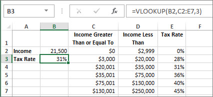
The fourth argument is empty, so the function returns an approximate match. If it didn’t, you’d have to enter one of the values in columns C or D to get a result at all.
When you’re comfortable with VLOOKUP, the HLOOKUP function is equally easy to use. You enter the same arguments, but it searches in rows instead of columns.
Using INDEX and MATCH instead of VLOOKUP
There are certain limitations with using VLOOKUP—the VLOOKUP function can only look up a value from left to right. This means that the column containing the value you look up should always be located to the left of the column containing the return value. Now if your spreadsheet isn’t built this way, then do not use VLOOKUP. Use the combination of INDEX and MATCH functions instead.
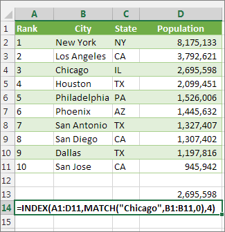
This example shows a small list where the value we want to search on, Chicago, isn’t in the leftmost column. So, we can’t use VLOOKUP. Instead, we’ll use the MATCH function to find Chicago in the range B1:B11. It’s found in row 4. Then, INDEX uses that value as the lookup argument, and finds the population for Chicago in the 4th column (column D). The formula used is shown in cell A14.
For more examples of using INDEX and MATCH instead of VLOOKUP, see the article https://www.mrexcel.com/excel-tips/excel-vlookup-index-match/ by Bill Jelen, Microsoft MVP.
Give it a try
If you want to experiment with lookup functions before you try them out with your own data, here’s some sample data.
VLOOKUP Example at work
Copy the following data into a blank spreadsheet.
Tip: Before you paste the data into Excel, set the column widths for columns A through C to 250 pixels, and click Wrap Text (Home tab, Alignment group).
|
Density |
Viscosity |
Temperature |
|
0.457 |
3.55 |
500 |
|
0.525 |
3.25 |
400 |
|
0.606 |
2.93 |
300 |
|
0.675 |
2.75 |
250 |
|
0.746 |
2.57 |
200 |
|
0.835 |
2.38 |
150 |
|
0.946 |
2.17 |
100 |
|
1.09 |
1.95 |
50 |
|
1.29 |
1.71 |
0 |
|
Formula |
Description |
Result |
|
=VLOOKUP(1,A2:C10,2) |
Using an approximate match, searches for the value 1 in column A, finds the largest value less than or equal to 1 in column A which is 0.946, and then returns the value from column B in the same row. |
2.17 |
|
=VLOOKUP(1,A2:C10,3,TRUE) |
Using an approximate match, searches for the value 1 in column A, finds the largest value less than or equal to 1 in column A, which is 0.946, and then returns the value from column C in the same row. |
100 |
|
=VLOOKUP(0.7,A2:C10,3,FALSE) |
Using an exact match, searches for the value 0.7 in column A. Because there is no exact match in column A, an error is returned. |
#N/A |
|
=VLOOKUP(0.1,A2:C10,2,TRUE) |
Using an approximate match, searches for the value 0.1 in column A. Because 0.1 is less than the smallest value in column A, an error is returned. |
#N/A |
|
=VLOOKUP(2,A2:C10,2,TRUE) |
Using an approximate match, searches for the value 2 in column A, finds the largest value less than or equal to 2 in column A, which is 1.29, and then returns the value from column B in the same row. |
1.71 |
HLOOKUP Example
Copy all the cells in this table and paste it into cell A1 on a blank worksheet in Excel.
Tip: Before you paste the data into Excel, set the column widths for columns A through C to 250 pixels, and click Wrap Text (Home tab, Alignment group).
|
Axles |
Bearings |
Bolts |
|
4 |
4 |
9 |
|
5 |
7 |
10 |
|
6 |
8 |
11 |
|
Formula |
Description |
Result |
|
=HLOOKUP(«Axles», A1:C4, 2, TRUE) |
Looks up «Axles» in row 1, and returns the value from row 2 that’s in the same column (column A). |
4 |
|
=HLOOKUP(«Bearings», A1:C4, 3, FALSE) |
Looks up «Bearings» in row 1, and returns the value from row 3 that’s in the same column (column B). |
7 |
|
=HLOOKUP(«B», A1:C4, 3, TRUE) |
Looks up «B» in row 1, and returns the value from row 3 that’s in the same column. Because an exact match for «B» is not found, the largest value in row 1 that is less than «B» is used: «Axles,» in column A. |
5 |
|
=HLOOKUP(«Bolts», A1:C4, 4) |
Looks up «Bolts» in row 1, and returns the value from row 4 that’s in the same column (column C). |
11 |
|
=HLOOKUP(3, {1,2,3;»a»,»b»,»c»;»d»,»e»,»f»}, 2, TRUE) |
Looks up the number 3 in the three-row array constant, and returns the value from row 2 in the same (in this case, third) column. There are three rows of values in the array constant, each row separated by a semicolon (;). Because «c» is found in row 2 and in the same column as 3, «c» is returned. |
c |
INDEX and MATCH Examples
This last example employs the INDEX and MATCH functions together to return the earliest invoice number and its corresponding date for each of five cities. Because the date is returned as a number, we use the TEXT function to format it as a date. The INDEX function actually uses the result of the MATCH function as its argument. The combination of the INDEX and MATCH functions are used twice in each formula – first, to return the invoice number, and then to return the date.
Copy all the cells in this table and paste it into cell A1 on a blank worksheet in Excel.
Tip: Before you paste the data into Excel, set the column widths for columns A through D to 250 pixels, and click Wrap Text (Home tab, Alignment group).
|
Invoice |
City |
Invoice Date |
Earliest invoice by city, with date |
|
3115 |
Atlanta |
4/7/12 |
=»Atlanta = «&INDEX($A$2:$C$33,MATCH(«Atlanta»,$B$2:$B$33,0),1)& «, Invoice date: » & TEXT(INDEX($A$2:$C$33,MATCH(«Atlanta»,$B$2:$B$33,0),3),»m/d/yy») |
|
3137 |
Atlanta |
4/9/12 |
=»Austin = «&INDEX($A$2:$C$33,MATCH(«Austin»,$B$2:$B$33,0),1)& «, Invoice date: » & TEXT(INDEX($A$2:$C$33,MATCH(«Austin»,$B$2:$B$33,0),3),»m/d/yy») |
|
3154 |
Atlanta |
4/11/12 |
=»Dallas = «&INDEX($A$2:$C$33,MATCH(«Dallas»,$B$2:$B$33,0),1)& «, Invoice date: » & TEXT(INDEX($A$2:$C$33,MATCH(«Dallas»,$B$2:$B$33,0),3),»m/d/yy») |
|
3191 |
Atlanta |
4/21/12 |
=»New Orleans = «&INDEX($A$2:$C$33,MATCH(«New Orleans»,$B$2:$B$33,0),1)& «, Invoice date: » & TEXT(INDEX($A$2:$C$33,MATCH(«New Orleans»,$B$2:$B$33,0),3),»m/d/yy») |
|
3293 |
Atlanta |
4/25/12 |
=»Tampa = «&INDEX($A$2:$C$33,MATCH(«Tampa»,$B$2:$B$33,0),1)& «, Invoice date: » & TEXT(INDEX($A$2:$C$33,MATCH(«Tampa»,$B$2:$B$33,0),3),»m/d/yy») |
|
3331 |
Atlanta |
4/27/12 |
|
|
3350 |
Atlanta |
4/28/12 |
|
|
3390 |
Atlanta |
5/1/12 |
|
|
3441 |
Atlanta |
5/2/12 |
|
|
3517 |
Atlanta |
5/8/12 |
|
|
3124 |
Austin |
4/9/12 |
|
|
3155 |
Austin |
4/11/12 |
|
|
3177 |
Austin |
4/19/12 |
|
|
3357 |
Austin |
4/28/12 |
|
|
3492 |
Austin |
5/6/12 |
|
|
3316 |
Dallas |
4/25/12 |
|
|
3346 |
Dallas |
4/28/12 |
|
|
3372 |
Dallas |
5/1/12 |
|
|
3414 |
Dallas |
5/1/12 |
|
|
3451 |
Dallas |
5/2/12 |
|
|
3467 |
Dallas |
5/2/12 |
|
|
3474 |
Dallas |
5/4/12 |
|
|
3490 |
Dallas |
5/5/12 |
|
|
3503 |
Dallas |
5/8/12 |
|
|
3151 |
New Orleans |
4/9/12 |
|
|
3438 |
New Orleans |
5/2/12 |
|
|
3471 |
New Orleans |
5/4/12 |
|
|
3160 |
Tampa |
4/18/12 |
|
|
3328 |
Tampa |
4/26/12 |
|
|
3368 |
Tampa |
4/29/12 |
|
|
3420 |
Tampa |
5/1/12 |
|
|
3501 |
Tampa |
5/6/12 |
Excel has a lot of functions – about 450+ of them.
And many of these are simply awesome. The amount of work you can get done with a few formulas still surprises me (even after having used Excel for 10+ years).
And among all these amazing functions, the INDEX MATCH functions combo stands out.
I am a huge fan of INDEX MATCH combo and I have made it pretty clear many times.
I even wrote an article about Index Match Vs VLOOKUP which sparked a little bit of debate (you can check the comments section for some firework).
And today, I am writing this article solely focussed on Index Match to show you some simple and advanced scenarios where you can use this powerful formula combo and get the work done.
Note: There are other lookup formulas in Excel – such as VLOOKUP and HLOOKUP and these are great. Many people find VLOOKUP to be easier to use (and that’s true as well). I believe INDEX MATCH is a better option in many cases. But since people find it difficult, it gets used less. So I am trying to simplify it using this tutorial.
Now before I show you how the combination of INDEX MATCH is changing the world of analysts and data scientists, let me first introduce you to the individual parts – INDEX and MATCH functions.
INDEX Function: Finds the Value-Based on Coordinates
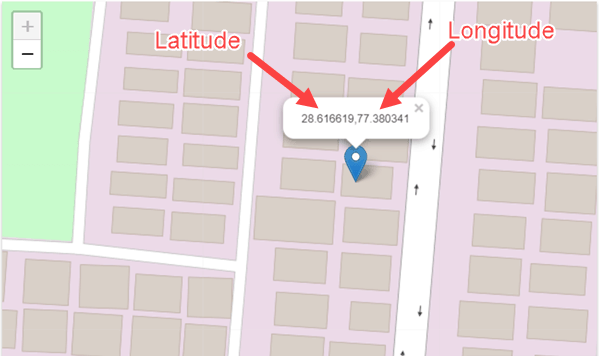
The easiest way to understand how Index function works is by thinking of it as a GPS satellite.
As soon as you tell the satellite the latitude and longitude coordinates, it will know exactly where to go and find that location.
So despite having a mind-boggling number of lat-long combinations, the satellite would know exactly where to look.
I quickly did a search for my work location and this is what I got.
Anyway, enough of geography.
Just like a satellite needs latitude and longitude coordinates, the INDEX function in Excel would need the row and column number to know what cell you’re referring to.
And that’s Excel INDEX function in a nut-shell.
So let me define it in simple words for you.
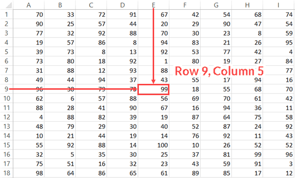
The INDEX function will use the row number and column number to find a cell in the given range and return the value in it.
All by itself, INDEX is a very simple function, with no utility. After all, in most cases, you are not likely to know the row and column numbers.
But…
The fact that you can use it with other functions (hint: MATCH) that can find the row number and the column number makes INDEX an extremely powerful Excel function.
Below is the syntax of the INDEX function:
=INDEX (array, row_num, [col_num])
=INDEX (array, row_num, [col_num], [area_num])
- array – a range of cells or an array constant.
- row_num – the row number from which the value is to be fetched.
- [col_num] – the column number from which the value is to be fetched. Although this is an optional argument, but if row_num is not provided, it needs to be given.
- [area_num] – (Optional) If array argument is made up of multiple ranges, this number would be used to select the reference from all the ranges.
INDEX function has 2 syntaxes (just FYI).
The first one is used in most cases. The second one is used in advanced cases only (such as doing a three-way lookup) which we will cover in one of the examples later in this tutorial.
But if you’re new to this function, just remember the first syntax.
Below is a video that explains how to use the INDEX function
MATCH Function: Finds the Position baed on a Lookup Value
Going back to my previous example of longitude and latitude, MATCH is the function that can find these positions (in the Excel spreadsheet world).
In simple language, the Excel MATCH function can find the position of a cell in a range.
And on what basis would it find a cell’s position?
Based on the lookup value.
For example, if you have a list as shown below and you want to find the position of the name ‘Mark’ in it, then you can use the MATCH function.
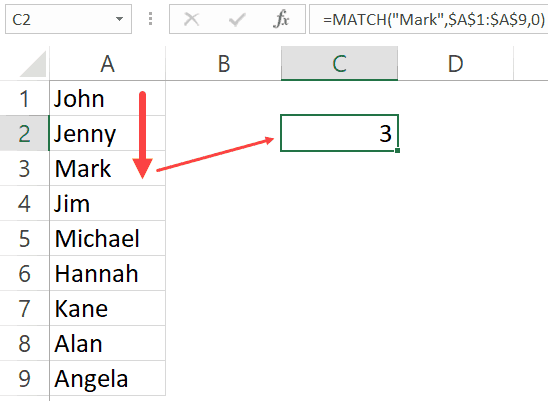
The function returns 3, as that’s the position of the cell with the name Mark in it.
MATCH function starts looking from top to bottom for the lookup value (which is ‘Mark’) in the specified range (which is A1:A9 in this example). As soon as it finds the name, it returns the position in that specific range.
Below is the syntax of the MATCH function in Excel.
=MATCH(lookup_value, lookup_array, [match_type])
- lookup_value – The value for which you are looking for a match in the lookup_array.
- lookup_array – The range of cells in which you are searching for the lookup_value.
- [match_type] – (Optional) This specifies how excel should look for a matching value. It can take three values -1, 0 , or 1.
Understanding Match Type Argument in MATCH Function
There is one additional thing you need to know about the MATCH function, and it’s about how it goes through the data and finds the cell position.
The third argument of the MATCH function can be 0, 1 or -1.
Below is an explanation of how these arguments work:
- 0 – this will look for an exact match of the value. If an exact match is found, the MATCH function will return the cell position. Else, it will return an error.
- 1 – this finds the largest value that is less than or equal to the lookup value. For this to work, your data range needs to be sorted in ascending order.
- -1 – this finds the smallest value that is greater than or equal to the lookup value. For this to work, your data range needs to be sorted in descending order.
Below is a video that explains how to use the MATCH function (along with the match type argument)
To summarize and put it in simple words:
- INDEX needs the cell position (row and column number) and gives the cell value.
- MATCH finds the position by using a lookup value.
Let’s Combine Them to Create a Powerhouse (INDEX + MATCH)
Now that you have a basic understanding of how INDEX and MATCH functions work individually, let’s combine these two and learn about all the wonderful things it can do.
To understand this better, I have a few examples that use the INDEX MATCH combination.
I will start with a simple example and then show you some advanced use cases as well.
Click here to download the example file
Example 1: A simple Lookup Using INDEX MATCH Combo
Let’s do a simple lookup with INDEX/MATCH.
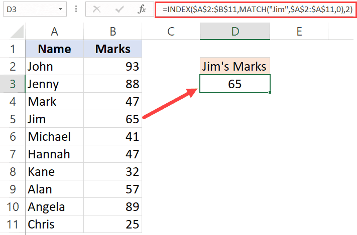
Below is a table where I have the marks for ten students.
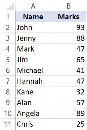
From this table, I want to find the marks for Jim.
Below is the formula that can easily do this:
=INDEX($A$2:$B$11,MATCH("Jim",$A$2:$A$11,0),2)
Now, if you’re thinking this can easily be done using a VLOOKUP function, you’re right! This is not the best use of INDEX MATCH awesomeness. Despite the fact that I am a fan of INDEX MATCH, it is a little more difficult than VLOOKUP. If fetching data from a column on the right is all you want to do, I recommend you use VLOOKUP.
The reason I have shown this example, which can also easily be done with VLOOKUP is to show you how INDEX MATCH works in a simple setting.
Now let me show a benefit of INDEX MATCH.
Suppose you have the same data, but instead of having it in columns, you have it in rows (as shown below).

You know what, you can still use INDEX MATCH combo to get Jim’s marks.
Below is the formula that will give you the result:
=INDEX($B$1:$K$2,2,MATCH(“Jim”,$B$1:$K$1,0))
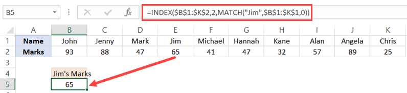
Note that you need to change the range and switch the row/column parts to make this formula work for horizontal data as well.
This can’t be done with VLOOKUP, but you can still do this easily with HLOOKUP.
INDEX MATCH combination can easily handle horizontal as well as vertical data.
Click here to download the example file
Example 2: Lookup to the Left
It’s more common than you think.
A lot of times, you may be required to fetch the data from a column which is to the left of the column that has the lookup value.
Something as shown below:
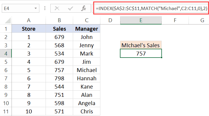
To find out Michael’s sales, you will have to do a lookup on the left.
If you’re thinking VLOOKUP, let me stop your right there.
VLOOKUP is not made to look for and fetch the values on the left.
Can you still do it using VLOOKUP?
Yes, you can!
But that can turn into a long and ugly formula.
So if you want to do a lookup and fetch data from the columns on the left, you are better off using INDEX MATCH combo.
Below is the formula that will get Michael’s sales number:
=INDEX($A$2:$C$11,MATCH("Michael",C2:C11,0),2)
Another point here for INDEX MATCH. VLOOKUP can fetch the data only from the columns that are to the right of the column that has the lookup value.
Example 3: Two Way Lookup
So far, we have seen the examples where we wanted to fetch the data from the column adjacent to the column that has the lookup value.
But in real life, the data often spans through multiple columns.
INDEX MATCH can easily handle a two-way lookup.
Below is a dataset of the student’s marks in three different subjects.
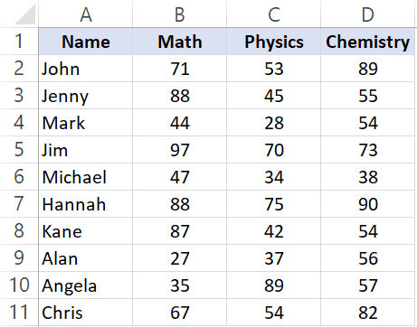
If you want to quickly fetch the marks of a student in all three subjects, you can do that with INDEX MATCH.
The below formula will give you the marks for Jim for all the three subjects (copy and paste in one cell and drag to fill other cells or copy and paste on other cells).
=INDEX($B$2:$D$11,MATCH($F$3,$A$2:$A$11,0),MATCH(G$2,$B$1:$D$1,0))

Let me quickly also explain this formula.
INDEX formula uses B2:D11 as the range.
The first MATCH uses the name (Jim in cell F3) and fetches the position of it in the names column (A2:A11). This becomes the row number from which the data needs to be fetched.
The second MATCH formula uses the subject name (in cell G2) to get the position of that specific subject name in B1:D1. For example, Math is 1, Physics is 2 and Chemistry is 3.
Since these MATCH positions are fed into the INDEX function, it returns the score based on the student name and subject name.
This formula is dynamic, which means that if you change the student name or the subject names, it would still work and fetch the correct data.
One great thing about using INDEX/MATCH is that even if you interchange the names of the subjects, it will continue to give you the correct result.
Example 4: Lookup Value From Multiple Column/Criteria
Suppose you have a dataset as shown below and you want to fetch the marks for ‘Mark Long’.

Since the data is in two columns, I can’t a lookup for Mark and get the data.
If I do it that way, I am going to get the marks data for Mark Frost and not Mark Long (because the MATCH function will give me the result for the MARK it meets).
One way of doing this is to create a helper column and combine the names. Once you have the helper column, you can use VLOOKUP and get the marks data.
If you’re interested in learning how to do this, read this tutorial on using VLOOKUP with multiple criteria.
But with INDEX/MATCH combo, you don’t need a helper column. You can create a formula that handles multiple criteria in the formula itself.
The below formula will give the result.
=INDEX($C$2:$C$11,MATCH($E$3&"|"&$F$3,$A$2:A11&"|"&$B$2:$B$11,0))

Let me quickly explain what this formula does.
The MATCH part of the formula combines the lookup value (Mark and Long) as well as the entire lookup array. When $A$2:A11&”|”&$B$2:$B$11 is used as the lookup array, it actually checks the lookup value against the combined string of first and last name (separated by the pipe symbol).
This ensures that you get the right result without using any helper columns.
You can do this kind of lookup (where there are multiple columns/criteria) with VLOOKUP as well, but you need to use a helper column. INDEX MATCH combo makes it slightly easy to do this without any helper columns.
Example 5: Get Values from Entire Row/Column
In the examples above, we have used the INDEX function to get value from a specific cell. You provide the row and column number, and it returns the value in that specific cell.
But you can do more.
You can also use the INDEX function to get the values from an entire row or column.
And how can this be useful you ask!
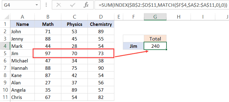
Suppose you want to know the total score of Jim in all the three subjects.
You can use the INDEX function to first get all the marks of Jim and then use the SUM function to get a total.
Let’s see how to do this.
Below I have the scores of all the students in three subjects.
The below formula will give me the total score of Jim in all the three subjects.
=SUM(INDEX($B$2:$D$11,MATCH($F$4,$A$2:$A$11,0),0))
Let me explain how this formula works.
The trick here is to use 0 as the column number.
When you use 0 as the column number in the INDEX function, it will return all the row values. Similarly, if you use 0 as the row number, it will return all the values in the column.
So the below part of the formula returns an array of values – {97, 70, 73}
INDEX($B$2:$D$11,MATCH($F$4,$A$2:$A$11,0),0)
If you just enter this above formula in a cell in Excel and hit enter, you will see a #VALUE! error. This is because it’s not returning a single value, but an array of value.
But don’t worry, the array of values are still there. You can check this by selecting the formula and press the F9 key. It will show you the result of the formula which in this case is an array of three value – {97, 70, 73}
Now, if you wrap this INDEX formula in the SUM function, it will give you the sum of all the marks scored by Jim.
You can also use the same to get the highest, lowest and average marks of Jim.
Just like we have done this for a student, you can also do this for a subject. For example, if you want the average score in a subject, you can keep the row number as 0 in the INDEX formula and it will give you all the column values of that subject.
Click here to download the example file
Example 6: Find the Student’s Grade (Approximate Match Technique)
So far, we have used the MATCH formula to get the exact match of the lookup value.
But you can also use it to do an approximate match.
Now, what the hell is Approximate Match?
Let me explain.
When you’re looking for stuff such as names or ids, you’re looking for an exact match. But sometimes, you need to know the range in which your lookup values lie. This is usually the case with numbers.
For example, as a class teacher, you may want to know what’s the grade of each student in a subject, and the grade is decided based on the score.
Below is an example, where I want the grade for all the students and the grading is decided based on the table on the right.
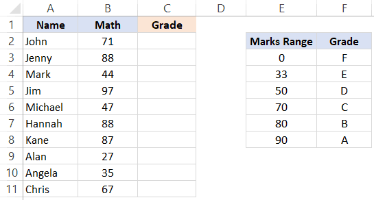
So if a student gets less than 33, the grade is F and if he/she gets less than 50 but more than 33, it’s E, and so on.
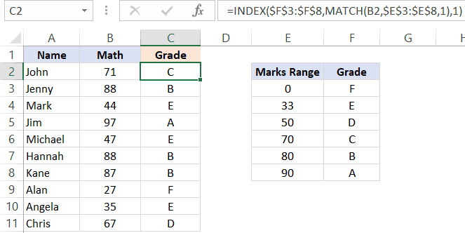
Below is the formula that will do this.
=INDEX($F$3:$F$8,MATCH(B2,$E$3:$E$8,1),1)
Let me explain how this formula works.
In the MATCH function, we have used 1 as the [match_type] argument. This argument will return the largest value that is less than or equal to the lookup value.
This means that the MATCH formula goes through the marks range, and as soon as it finds a marks range that is equal to or less than the lookup marks value, it will stop there and return its position.
So if the lookup mark value is 20, the MATCH function would return 1 and if it’s 85, it would return 5.
And the INDEX function uses this position value to get the grade.
IMPORTANT: For this to work, your data needs to be sorted in ascending order. If it’s not, you can get wrong results.
Note that the above can also be done using below VLOOKUP formula:
=VLOOKUP(B2,$E$3:$F$8,2,TRUE)
But MATCH function can go a step further when it comes to approximate match.
You can also have a descending data and can use INDEX MATCH combo to find the result. For example, if I change the order of the grade table (as shown below), I can still find the grades of the students.
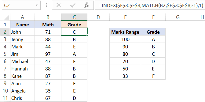
To do this, all I have to do is change the [match_type] argument to -1.
Below is the formula that I have used:
=INDEX($F$3:$F$8,MATCH(B2,$E$3:$E$8,-1),1)
VLOOKUP can also do an approximate match but only when data is sorted in ascending order(but it doesn’t work if the data is sorted in descending order).
Example 7: Case Sensitive Lookups
So far all the lookups we have done have been case insensitive.
This means that whether the lookup value was Jim or JIM or jim, it didn’t matter. You’ll get the same result.
But what if you want the lookup to be case sensitive.
This is usually the case when you have large data sets and a possibility of repetition or distinct names/ids (with the only difference being the case)
For example, suppose I have the following data set of students where there are two students with the name Jim (the only difference being that one is entered as Jim and another one as jim).

Note that there are two students with the same name – Jim (cell A2 and A5).
Since a normal lookup wouldn’t work, you need to do a case sensitive lookup.
Below is the formula that will give you the right result. Since this is an array formula, you need to use Control + Shift + Enter.
=INDEX($B$2:$B$11,MATCH(TRUE,EXACT(D3,A2:A11),0),1)

Let me explain how this formula works.
The EXACT function checks for an exact match of the lookup value (which is ‘jim’ in this case). It goes through all the names and returns FALSE if it isn’t a match and TRUE if it’s a match.
So the output of the EXACT function in this example is – {FALSE;FALSE;FALSE;TRUE;FALSE;FALSE;FALSE;FALSE;FALSE;FALSE}
Note that there is only one TRUE, which is when the EXACT function found a perfect match.
The MATCH function then finds the position of TRUE in the array returned by the EXACT function, which is 4 in this example.
Once we have the position, the INDEX function uses it to find the marks.
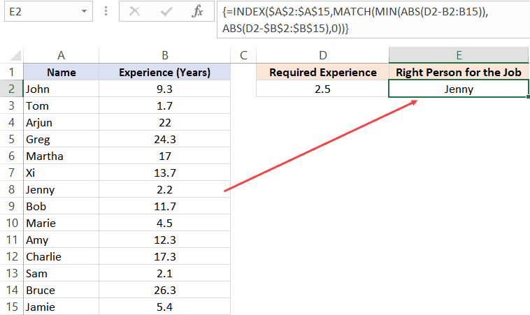
Example 8: Find the Closest Match
Let’s get a little advanced now.
Suppose you have a dataset where you want to find the person who has the work experience closest to the required experience (mentioned in cell D2).
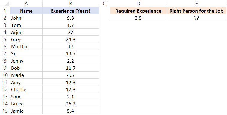
While lookup formulas are not made to do this, you can combine it with other functions (such as MIN and ABS) to get this done.
Below is the formula that will find the person with the experience closest to the required one and return the name of the person. Note that the experience needs to be closest (which can be either less or more).
=INDEX($A$2:$A$15,MATCH(MIN(ABS(D2-B2:B15)),ABS(D2-$B$2:$B$15),0))
Since this is an array formula, you need to use Control + Shift + Enter.
The trick in this formula is to change the lookup value and lookup array to find the minimum experience difference in required and actual values.
Before I explain the formula, let’s understand how you would do it manually.
You will go through each cell in column B and find the difference in the experience between what is required and the one that a person has. Once you have all the differences, you will find the one which is minimum and fetch the name of that person.
This is exactly what we are doing with this formula.
Let me explain.
The lookup value in the MATCH formula is MIN(ABS(D2-B2:B15)).
This part gives you the minimum difference between the given experience (which is 2.5 years) and all the other experiences. In this example, it returns 0.3
Note that I have used ABS to make sure I am looking for the closest (which can be more or less than the given experience).
Now, this minimum value becomes our lookup value.
The lookup array in the MATCH function is ABS(D2-$B$2:$B$15).
This gives us an array of numbers from which 2.5 (the required experience) has been subtracted.
So now we have a lookup value (0.3) and a lookup array ({6.8;0.8;19.5;21.8;14.5;11.2;0.3;9.2;2;9.8;14.8;0.4;23.8;2.9})
MATCH function finds the position of 0.3 in this array, which is also the position of the person’s name who has the closest experience.
This position number is then used by the INDEX function to return the name of the person.
Related Read: Find the Closest Match in Excel (examples using lookup formulas)
Click here to download the example file
Example 9: Use INDEX MATCH with Wildcard Characters
If you want to look up a value when there is a partial match, then you need to use wildcard characters.
For example, below is a dataset of company name and their market capitalizations and you want to want to get the market cap. data for the three companies on the right.
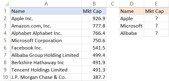
Since these are not exact matches, you can’t do a regular lookup in this case.
But you can still get the right data by using an asterisk (*), which is a wildcard character.
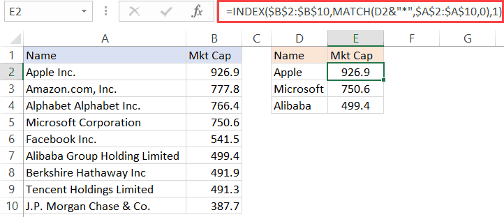
Below is the formula that will give you the data by matching the company names from the main column and fetching the market cap figure for it.
=INDEX($B$2:$B$10,MATCH(D2&”*”,$A$2:$A$10,0),1)
Let me explain how this formula works.
Since there is no exact match of lookup values, I have used D2&”*” as the lookup value in the MATCH function.
An asterisk is a wildcard character that represents any number of characters. This means that Apple* in the formula would mean any text string that starts with the word Apple and can have any number of characters after it.
So when Apple* is used as the lookup value and the MATCH formula looks for it in column A, it returns the position of ‘Apple Inc.’, as it starts with the word Apple.
You can also use wildcard characters to find text strings where the lookup value is in between. For example, if you use *Apple* as the lookup value, it will find any string that has the word apple anywhere in it.
Note: This technique works well when you only have one instance of matching. But if you have multiple instances of matching (for example Apple Inc and Apple Corporation, then the MATCH function would return the position of the first matching instance only.
Example 10: Three Way Lookup
This is an advanced use of INDEX MATCH, but I will still cover it to show you the power of this combination.
Remember I said that INDEX function has two syntaxes:
=INDEX (array, row_num, [col_num])
=INDEX (array, row_num, [col_num], [area_num])
So far in all our examples, we have only used the first one.
But for a three-way lookup, you need to use the second syntax.
Let me first explain what a three-way look means.
In a two-way lookup, we use the INDEX MATCH formula to get the marks when we have the student’s name and the subject name. For example, fetching the marks of Jim in Math is a two-way lookup.
A three-way look would add another dimension to it. For example, suppose you have a dataset as shown below and you want to know the score of Jim in Math in Mid-term exam, then this would be three-way lookup.
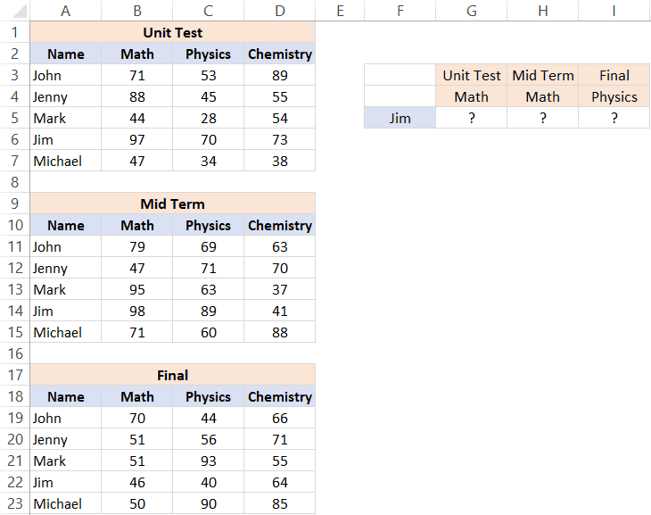
Below is the formula that will give the result.
=INDEX(($B$3:$D$7,$B$11:$D$15,$B$19:$D$23),MATCH($F$5,$A$3:$A$7,0),MATCH(G$4,$B$2:$D$2,0),(IF(G$3="Unit Test",1,IF(G$3="Mid Term",2,3))))
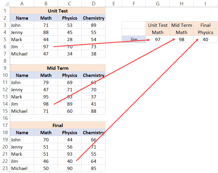
The above formula checked for three things – the name of the student, the subject, and the exam. After it finds the right value, it returns it in the cell.
Let me explain how this formula works by breaking down the formula into parts.
- array – ($B$3:$D$7,$B$11:$D$15,$B$19:$D$23): Instead of using a single array, in this case, I have used three arrays within parenthesis.
- row_num – MATCH($F$5,$A$3:$A$7,0): MATCH function is used to find the position of the student’s name in cell $F$5 in the list of student’s name.
- col_num – MATCH(G$4,$B$2:$D$2,0): MATCH function is used to find the position of the subject name in cell $B$2 in the list of subject’s name.
- [area_num] – IF(G$3=”Unit Test”,1,IF(G$3=”Mid Term”,2,3)): The area number value tells the INDEX function which of the three arrays to use to fetch the value. If the exam is Unit Term, the IF function would return 1 and the INDEX function would use the first array to fetch the value. If the exam is Mid-term, the IF formula would return 2, else it will return 3.
This is an advanced example of using INDEX MATCH, and you’re unlikely to find a situation when you have to use this. But it’s still good to know what Excel formulas can do.
Click here to download the example file
Why is INDEX/MATCH Better than VLOOKUP?
OR Is it?
Yes, it is – in most cases.
I will present my case in a while.
But before I do that, let me say this – VLOOKUP is an extremely useful function and I love it. It can do a lot of things in Excel and I use it every now and then myself. Having said that, it doesn’t mean that there can’t be anything better, and INDEX/MATCH (with more flexibility and functionalities) is better.
So if you want to do some basic lookup, you’re better off using VLOOKUP.
INDEX/MATCH is VLOOKUP on steroids. And once you learn INDEX/MATCH, you might always prefer using it (especially because of the flexibility it has).
Without stretching it too far, let me quickly give you the reasons why INDEX/MATCH is better than VLOOKUP.
INDEX/MATCH can look to the Left (as well as to the right) of the lookup value
I covered it in one of the example above.
If you have a value which is on the left of the lookup value, you can’t do that with VLOOKUP
At least not with just VLOOKUP.
Yes, you can combine VLOOKUP with other formulas and get it done, but it gets complicated and messy.
INDEX/MATCH, on the other hand, is made to lookup everywhere (be it left, right, up, or down)
INDEX/MATCH can work with vertical and horizontal ranges
Again, with full respect to VLOOKUP, it’s not made to do this.
After all, the V in VLOOKUP stands for vertical.
VLOOKUP can only go through data that is vertical, while INDEX/MATCH can go through data vertically as well horizontally.
Of course, there is the HLOOKUP function to take care of horizontal lookup, but it isn’t VLOOKUP then.. right?
I like the fact that INDEX MATCH combo is flexible enough to work with both vertical and horizontal data.
VLOOKUP cannot work with descending data
When it comes to the approximate match, VLOOKUP and INDEX/MATCH are at the same level.
But INDEX MATCH takes the point as it can also handle data that is in descending order.
I show this in one of the examples in this tutorial where we have to find the grade of students based on the grading table. If the table is sorted in descending order, VLOOKUP would not work (but INDEX MATCH would).
INDEX/MATCH can be slightly faster
I will be truthful. I didn’t run this test myself.
I am relying on the wisdom an Excel master – Charley Kyd.
The difference in speed in VLOOKUP and INDEX/MATCH is hardly noticeable when you have small data sets. But if you have thousands of rows and many columns, this can be a deciding factor.
In his article, Charley Kyd states:
“At its worst, the INDEX-MATCH method is about as fast as VLOOKUP; at its best, it’s much faster.”
INDEX/MATCH is Independent of the Actual Column Position
If you have a dataset as shown below as you’re fetching the score of Jim in Physics, you can do that using VLOOKUP.
And to do that, you can specify the column number as 3 in VLOOKUP.
All is fine.
But what if I delete the Math column.
In that case, the VLOOKUP formula will break.
Why? – Because it was hardcoded to use the third column, and when I delete a column in between, the third column becomes the second column.
Using INDEX/MATCH, in this case, is better as you can make the column number dynamic by using MATCH. So instead of a column number, it checks for the subject name and uses that to return the column number.
Surely you can do that by combining VLOOKUP with MATCH, but if you combining anyway, why not do it with INDEX which is a lot more flexible.
When using INDEX/MATCH, you can safely insert/delete columns in your dataset.
Despite all these factors, there is a reason VLOOKUP is so popular.
And it’s a big reason.
VLOOKUP is easier to use
VLOOKUP only takes a maximum of four arguments. If you can wrap your head around these four, you’re good to go.
And since most of the basic lookup cases are handled by VLOOKUP as well, it has quickly become the most popular Excel function.
I call it the King of Excel functions.
INDEX/MATCH, on the other hand, is a little more difficult to use. You may get a hang if it when you start using it, but for a beginner, VLOOKUP is far more easy to explain and learn.
And this is not a zero-sum game.
So, if you’re new to the lookup world and don’t know how to use VLOOKUP, better learn that.
I have a detailed guide on using VLOOKUP in Excel (with lots of examples)
My intent in this article is not to pitch two awesome functions against each other. I wanted to show you the power of INDEX MATCH combo and all the great things it can do.
Hope you found this article useful.
Let me know your thoughts in the comments section, and in case you find any mistake in this tutorial, please let me know.
You May Also Like the Following Excel Tutorials:
- Excel Functions
- 100+ Excel Interview Questions
- Find the Last Occurrnece of a Lookup Value in a List
- Lookup the Second, the Third, or the Nth Value in Excel
- Use IFERROR with VLOOKUP to Get Rid of #N/A Errors
How to combine INDEX, MATCH, and MATCH formulas in Excel as a lookup function
What is INDEX MATCH in Excel?
The INDEX MATCH[1] Formula is the combination of two functions in Excel: INDEX[2] and MATCH[3].
=INDEX() returns the value of a cell in a table based on the column and row number.
=MATCH() returns the position of a cell in a row or column.
Combined, the two formulas can look up and return the value of a cell in a table based on vertical and horizontal criteria. For short, this is referred to as just the Index Match function. To see a video tutorial, check out our free Excel Crash Course.
#1 How to Use the INDEX Formula
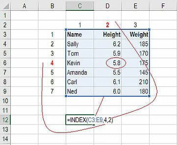
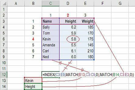
Below is a table showing people’s names, height, and weight. We want to use the INDEX formula to look up Kevin’s height… here is an example of how to do it.
Follow these steps:
- Type “=INDEX(” and select the area of the table, then add a comma
- Type the row number for Kevin, which is “4,” and add a comma
- Type the column number for Height, which is “2,” and close the bracket
- The result is “5.8.”
#2 How to Use the MATCH Formula
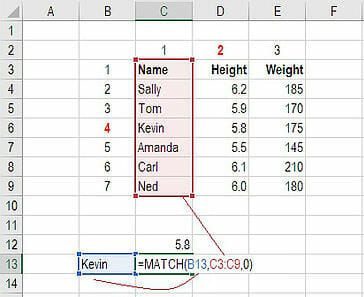
Sticking with the same example as above, let’s use MATCH to figure out what row Kevin is in.
Follow these steps:
- Type “=MATCH(” and link to the cell containing “Kevin”… the name we want to look up.
- Select all the cells in the Name column (including the “Name” header).
- Type zero “0” for an exact match.
- The result is that Kevin is in row “4.”
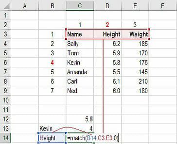
Use MATCH again to figure out what column Height is in.
Follow these steps:
- Type “=MATCH(” and link to the cell containing “Height”… the criteria we want to look up.
- Select all the cells across the top row of the table.
- Type zero “0” for an exact match.
- The result is that Height is in column “2.”
#3 How to Combine INDEX and MATCH
Now we can take the two MATCH formulas and use them to replace the “4” and the “2” in the original INDEX formula. The result is an INDEX MATCH formula.
Follow these steps:
- Cut the MATCH formula for Kevin and replace the “4” with it.
- Cut the MATCH formula for Height and replace the “2” with it.
- The result is Kevin’s Height is “5.8.”
- Congratulations, you now have a dynamic INDEX MATCH formula!
Video Explanation of How to Use Index Match in Excel
Below is a short video tutorial on how to combine the two functions and effectively use Index Match in Excel! Check out more free Excel tutorials on CFI’s YouTube Channel.
Hopefully, this short video made it even clearer how to use the two functions to dramatically improve your lookup capabilities in Excel.
More Excel Lessons
Thank you for reading this step-by-step guide to using INDEX MATCH in Excel. To continue learning and advancing your skills, these additional CFI resources will be helpful:
- Free Excel Fundamentals Course
- Excel Formulas and Functions List
- Excel Shortcuts
- Go To Special
- Find and Replace
- IF AND Function in Excel
- See all Excel resources
How to Use INDEX MATCH
With Multiple Criteria in Excel
INDEX MATCH with multiple criteria enables you to do a successful lookup when there are multiple lookup value matches.
In other words, you can look up and return values even if there are no unique values to look for.
This is not achievable with any other lookup formula without inserting helper columns😲
Follow these 3 easy steps to create your very own INDEX MATCH with multiple criteria in a few minutes.
If you want to tag along, download the sample Excel file here.
INDEX MATCH with multiple criteria example
So, you got this employee database.

You want to make the database easier to search, so you’re creating a small tool (to the right).
In that tool, anyone should be able to type in the name and division of an employee and it will find that person’s salary (and show it in cell G4).
“That’s easy, I can just use VLOOKUP.”
Wait a minute✋
Unfortunately, it’s not that easy.
You see, the problem is that there are actually 2 employees called “Steve Jones”. That means the lookup value has 2 matches in the lookup column.

There’s nothing unique about Steve Jones’ name on its own.
In Excel terminology, ‘Name’ would be 1 criteria.
So, 1 criteria didn’t cut it.
But if you include another criteria, like ‘Division’, you make Steve Jones unique.

Now, while “Steve Jones” appears several times on the list, there’s only one “Steve Jones from the sales division”.
This is the kind of magic you can do with INDEX MATCH with multiple criteria.
Step 1: Insert a normal INDEX MATCH formula
INDEX MATCH with multiple criteria is an ‘array formula’ created from the INDEX and MATCH functions.
An array formula has a syntax that is different from normal formulas. It’s basically a normal formula on steroids💪
The synergies between the INDEX and MATCH functions are that:
- MATCH searches for a value and returns a location
- MATCH feeds the location to the INDEX function
- Then INDEX transforms this location into a result

Start with:
=MATCH(
1. As the first argument in the MATCH function, enter the lookup value. This is what you are looking for.
In this case, you’re looking for an employee with the name “Steve Jones”.
Select (or manually enter) cell G2 as lookup value, then separate with a comma to move on to the lookup array.

2. The lookup array is the column where the MATCH function looks for the lookup value.
Select the column with the names, and then enter a comma to move on to the [match_type].

Now your formula should look like this:
=MATCH(G2,A:A,
3. A little drop-down list appears that gives you the choice between 1, 0, and -1.

The 0 option is the “exact match” option and is most commonly used. The -1 and 1 are similar to VLOOKUP’s “approximate match” method.
Write 0 or double-click the ‘0 – Exact match’ option in the drop-down menu and type the end parenthesis.

Your formula should now look like this:
=MATCH(G2,A:A,0)
4. Wrap the INDEX function around the MATCH function.

Your formula should look like this by now:
=INDEX(MATCH(G2,A:A,0)
But we’re not done yet✋
The syntax of the INDEX function goes:
INDEX(array, row number, column number)
The MATCH function should be the 2nd argument in the INDEX syntax.
Right now, it’s the 1st argument.
So, begin writing the real 1st argument: the array.
The INDEX array is the column you want to return values from.
The purpose of the multiple criteria INDEX MATCH is to find the salary of a specific employee.
So, the array is the salary column (column D).

Your formula should look like this by now:
=INDEX(D:D,MATCH(G2,A:A,0)
And just put an extra parenthesis at the end to wrap up the INDEX function.
So, the final formula looks like this:
=INDEX(D:D,MATCH(G2,A:A,0))
EXPLANATION
The MATCH function searches for the value in G2 (“Steve Jones”) in the database and then returns a number.
This number is the row in the data where the name “Steve Jones” is found.
This row number is then fed into the syntax of the INDEX function.
Problem: There’s more than one employee called “Steve Jones”. Whose salary are we actually seeing?
Excel lookup formulas always search from top to bottom, so you’re seeing the salary of the top Steve Jones (in row 3).
That’s the Steve you’re looking for.
But it’s dumb luck that you found him🍀
To make sure we always find Steve Jones from sales, follow the rest of the steps below.
Step 2: Change the lookup value to 1
Now, you need to change your normal INDEX MATCH formula into an array formula.
Sounds hard?
Don’t worry, I’ll guide you step-by-step😊
1. Change the lookup value of the MATCH function to 1. It’s just as easy as it sounds.

So, the formula changes from:
=INDEX(D:D,MATCH(G2,A:A,0))
To:
=INDEX(D:D,MATCH(1,A:A,0))
The “theory” behind this is not as simple as changing the lookup value.
Since you’re changing the formula from a normal one to an array formula, the structure of the formula changes a bit as well. By changing the lookup value to 1, you’re not actually telling the MATCH function to search for the number 1 in the lookup array (last name column).
In Excel-language, 1 means TRUE. 0 means FALSE.
When you enter our two criteria in the next step, the 1 in the MATCH function simply means:
“Look through the rows in the data and return the row number where all of the criteria are TRUE”.
If you wrote a zero, the formula would look for a row where all of our criteria are FALSE – and that wouldn’t really make sense.
Step 3: Write the criteria
The criteria replaces the 2nd argument of the MATCH function, with this structure:
(range=criteria1)*(range=criteria2)*(range=criteria3)*…
This way, you can have as many criteria as you need.
INDEX MATCH with 2 criteria
It’s typically enough to use 2 criteria to make your lookup value unique.
Criteria 1 = name
Criteria 2 = division
Let’s see if you can find “Steve Jones from sales” or if he’s lost in the woods🌳
Replace the structure above with the actual criteria:
(range=criteria1)*(range=criteria2)
(A:A=G2)*(B:B=G3)
A:A is the column with names. G2 is the name you’re looking for.
B:B is the column with division. G3 is the division you’re looking for.
Write that as the 2nd argument in the MATCH function, replacing what’s currently there.

Your formula should now look like this:
=INDEX(D:D,MATCH(1,(A:A=G2)*(B:B=G3),0))
It seems weird typing random parenthesis’ into formulas, but this is how you structure the criteria, so the array formula understands it.
If you’re using Microsoft 365 just press Enter and watch your beautiful multiple criteria lookup💡
Explanation: Ctrl + Shift + Enter
If you’re not using Microsoft 365, do not press Enter when you’re done with the formula. It won’t work.
Instead, press and hold Ctrl and Shift and then press Enter.
Warning: {curly brackets} will appear around your formula. They are supposed to be there!
Every time you make changes to this formula, you must end with Ctrl + Shift + Enter
(Instead of just regular “Enter” as you are probably used to)
That’s it – Now what?
Wow… You just learned how to use INDEX MATCH with multiple criteria…
It wasn’t so scary after all, right? 😎
Now, you’ve created a tool to easily look up employees and return their salary – even if there are multiple employees with the exact same name!
All fueled by the INDEX and MATCH functions.

Lookup formulas (and functions) in general are extremely useful and significantly speed up your work🏃
But multiple criteria lookups really save your day when the lookup value is not unique.
But if you really want to work more productively in Excel, you need to dive into macros.
Macros automate work processes, so you can do 50 things with just one click.
I promise you, it’s not as hard as you think.
Join my free 30-minute video course and get started with macros (for beginners).
Other relevant resources
INDEX MATCH is not the only lookup formula out there, although it’s the only one you can turn into an array formula. If you want to expand your toolbox you should definitely get to know VLOOKUP and the new XLOOKUP.
If you thought this was hard to understand, you should dive into the INDEX function and the MATCH function separately and get to know them better.
Another way to achieve a lookup with multiple criteria is with the good old Excel filter.
I hope this helps you!
Take care👋
Kasper Langmann2022-08-04T10:56:45+00:00
Page load link
Многие пользователи знают и применяют формулу ВПР. Известно также, что ВПР имеет ряд особенностей и ограничений, которые несложно обойти. Однако есть нюанс, который значительно ограничивает возможности функции ВПР.
ВПР требует, чтобы в диапазоне с искомыми данными столбец критериев всегда был первым слева. Это обстоятельство, конечно, является ограничением ВПР. Как же быть, если искомые данные находятся левее столбца с критерием? Можно, конечно, расположить столбцы в нужном порядке, что в целом, является неплохим выходом из ситуации. Но бывает так, что сделать этого нельзя, или трудно. К примеру, вы работаете в чужом документе или регулярно получаете новый отчет. В общем, нужно решение, не зависящее от расположения столбцов. Такое решение существует.
Нужно воспользоваться комбинацией из двух функций: ИНДЕКС и ПОИСКПОЗ. Формула работает следующим образом. ИНДЕКС отсчитывает необходимое количество ячеек вниз в диапазоне искомых значений. Количество отсчитываемых ячеек определяется по столбцу критериев функцией ПОИСКПОЗ. Работу комбинации этих функций удобно рассмотреть с середины, где вначале находится номер ячейки с подходящим критерием, а затем этот номер подставляется в ИНДЕКС.

Таким образом, чтобы подтянуть значение цены, соответствующее первому коду (книге), нужно прописать такую формулу.

Следует обратить внимание на корректность ссылок, чтобы при копировании формулы ничего не «съехало». Протягиваем формулу вниз. Если в таблице, откуда подтягиваются данные, нет искомого критерия, то функция выдает ошибку #Н/Д.

Довольно стандартная ситуация, с которой успешно справляется функция ЕСЛИОШИБКА. Она перехватывает ошибки и вместо них выдает что-либо другое, например, нули.
Конструкция формулы будет следующая:

Вот, собственно, и все.
Таким образом, комбинация функций ИНДЕКС и ПОИСКПОЗ является полной заменой ВПР и обладает дополнительным преимуществом: умеет находить данные слева от столбца с критерием. Кроме того, сами столбцы можно двигать как угодно, лишь бы ссылка не съехала, чего нельзя проделать с ВПР, т.к. количество столбцов там указывается конкретным числом. Посему комбинация ИНДЕКС и ПОИСКПОЗ более универсальна, чем ВПР.
Ниже видеоурок по работе функций ИНДЕКС и ПОИСКПОЗ.
Скачать файл с примером.
Поделиться в социальных сетях:
In this article, we will learn how to Lookup & SUM values with INDEX and MATCH function in Excel.
For the formula to understand first we need to revise a little about the three functions
- SUM
- INDEX
- MATCH
SUM function adds all the numbers in a range of cells and returns the sum of these values.
INDEX function returns the value at a given index in an array.
MATCH function returns the index of the first appearance of the value in an array ( single dimension array ).
Now we will make a formula using the above functions. Match function will return the index of the lookup value in the header field. The index number will now be fed to the INDEX function to get the values under the lookup value.
Then the SUM function will return the sum from the found values.
Use the Formula:
= SUM ( INDEX ( data , 0, MATCH ( lookup_value, headers, 0)))
The above statements can be complicated to understand. So let’s understand this by using the formula in an example
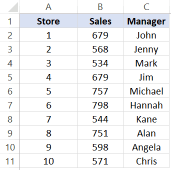
Here we have a list of marks of students and we need to find the total marks for a specific person (Gary) as shown in the snapshot below.
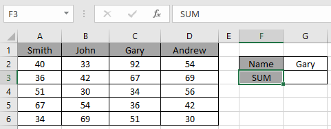
Use the formula in the C2 cell:
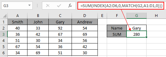
= SUM ( INDEX ( A2:D6 , 0 , MATCH ( G2 , A1:D1 , 0 )))
Explanation:
- The MATCH function matches the first value with the header array and returns its position 3 as a number.
- The INDEX function takes the number as the column index for the data and returns the array { 92 ; 67 ; 34 ; 36 ; 51 } to the argument of the SUM function
- The SUM function takes the array and returns the SUM in the cell.
Here values to the function is given as cell reference.
As you can see in the above snapshot, we got the SUM of the marks of student Gary. And it proves the formula works fine and for doubts see the below notes for understanding.
Notes:
- The function returns the #NA error if the lookup array argument to the MATCH function is 2 — D array which is the header field of the data..
- The function matches exact value as the match type argument to the MATCH function is 0.
- The lookup value can be given as cell reference or directly using quote symbol («).
- The SUM function ignores the text values in the array received from the INDEX function.
Hope you understood how to use the LOOKUP function in Excel. Explore more articles on Excel lookup value here. Please feel free to state your queries below in the comment box. We will certainly help you.
Related Articles
Use INDEX and MATCH to Lookup Value
SUM range with INDEX in Excel
How to use the SUM function in Excel
How to use the INDEX function in Excel
How to use the MATCH function in Excel
How to use LOOKUP function in Excel
How to use the VLOOKUP function in Excel
How to use the HLOOKUP function in Excel
Popular Articles
Edit a dropdown list
If with conditional formatting
If with wildcards
Vlookup by date
Skip to content
В этом руководстве показано, как использовать ИНДЕКС и ПОИСКПОЗ в Excel и чем они лучше ВПР.
В нескольких недавних статьях мы приложили немало усилий, чтобы объяснить основы функции ВПР новичкам и предоставить более сложные примеры формул ВПР опытным пользователям. А теперь я постараюсь если не отговорить вас от использования ВПР, то хотя бы показать вам альтернативный способ поиска нужных значений в Excel.
- Краткий обзор функций ИНДЕКС и ПОИСКПОЗ
- Как использовать формулу ИНДЕКС ПОИСКПОЗ
- ИНДЕКС+ПОИСКПОЗ вместо ВПР?
- Поиск справа налево
- Двусторонний поиск в строках и столбцах
- ИНДЕКС ПОИСКПОЗ для поиска по нескольким условиям
- Как найти среднее, максимальное и минимальное значение
- Что делать с ошибками поиска?
Для чего это нужно? Потому что функция ВПР имеет множество ограничений, которые могут помешать вам получить желаемый результат во многих ситуациях. С другой стороны, комбинация ПОИСКПОЗ ИНДЕКС более гибкая и имеет много замечательных возможностей, которые во многих отношениях превосходят ВПР.
Функции Excel ИНДЕКС и ПОИСКПОЗ — основы
Поскольку целью этого руководства является демонстрация альтернативного способа выполнения поиска в Excel с использованием комбинации функций ИНДЕКС и ПОИСКПОЗ, мы не будем подробно останавливаться на их синтаксисе и использовании. Тем более, что это подробно рассмотрено в других статьях, ссылки на которые вы можете найти в конце этого руководства. Мы рассмотрим лишь минимум, необходимый для понимания общей идеи, а затем подробно рассмотрим примеры формул, раскрывающие все преимущества использования ПОИСКПОЗ и ИНДЕКС вместо ВПР.
Функция ИНДЕКС
Функция ИНДЕКС (в английском варианте – INDEX) возвращает значение в массиве на основе указанных вами номеров строк и столбцов. Синтаксис функции ИНДЕКС прост:
ИНДЕКС(массив,номер_строки,[номер_столбца])
Вот простое объяснение каждого параметра:
- массив — это диапазон ячеек, именованный диапазон или таблица.
- номер_строки — это номер строки в массиве, из которого нужно вернуть значение. Если этот аргумент опущен, требуется следующий – номер_столбца.
- номер_столбца — это номер столбца, из которого нужно вернуть значение. Если он опущен, требуется номер_строки.
Дополнительные сведения см. в статье Функция ИНДЕКС в Excel .
А вот пример формулы ИНДЕКС в самом простом виде:
=ИНДЕКС(A1:C10;2;3)
Формула выполняет поиск в ячейках с A1 по C10 и возвращает значение ячейки во 2-й строке и 3-м столбце, т. е. в ячейке C2.
Очень легко, правда? Однако при работе с реальными данными вы вряд ли когда-нибудь будете заранее знать, какие строки и столбцы вам нужны. Здесь вам пригодится ПОИСКПОЗ.
Функция ПОИСКПОЗ
Она ищет нужное значение в диапазоне ячеек и возвращает относительное положение этого значения в диапазоне.
Синтаксис функции ПОИСКПОЗ следующий:
ПОИСКПОЗ(искомое_значение, искомый_массив, [тип_совпадения])
- искомое_значение — числовое или текстовое значение, которое вы ищете.
- диапазон_поиска — диапазон ячеек, в которых будем искать.
- тип_совпадения — указывает, следует ли искать точное соответствие или наиболее близкое совпадение:
- 1 или опущено — находит наибольшее значение, которое меньше или равно искомому значению. Требуется сортировка массива поиска в порядке возрастания.
- 0 — находит первое значение, точно равное искомому значению. В комбинации ИНДЕКС/ПОИСКПОЗ вам почти всегда нужно точное совпадение, поэтому вы чаще всего устанавливаете третий аргумент вашей функции в 0.
- -1 — находит наименьшее значение, которое больше или равно искомому значению. Требуется сортировка массива поиска в порядке убывания.
Например, если диапазон B1:B3 содержит значения «яблоки», «апельсины», «лимоны», приведенная ниже формула возвращает число 3, поскольку «лимоны» — это третья по счету запись в этом диапазоне:
=ПОИСКПОЗ(«лимоны»;B1:B3;0)
Дополнительные сведения см . в статье Функция ПОИСКПОЗ в Excel .
На первый взгляд полезность функции ПОИСКПОЗ может показаться сомнительной. Кого волнует положение значения в диапазоне? Что мы действительно хотим определить, так это само значение.
Однако, относительная позиция искомого значения (т. е. номера строки и столбца, в которых оно находится) — это именно то, что нам нужно указать для аргументов номер_строки и номер_столбца функции ИНДЕКС. Как вы помните, ИНДЕКС может найти значение на пересечении заданной строки и столбца, но сама не может определить, какую именно строку и столбец ей нужно выбрать.
Вот поэтому совместное использование ИНДЕКС и ПОИСКПОЗ открывает перед нами массу возможностей для поиска в Excel.
Как использовать формулу ИНДЕКС ПОИСКПОЗ в Excel
Теперь, когда вы знаете основы, я считаю, что вы уже начали понимать, как ПОИСКПОЗ и ИНДЕКС работают вместе. Короче говоря, ИНДЕКС извлекает нужное значение по номерам столбцов и строк, а ПОИСКПОЗ предоставляет ей эти номера. Вот и все!
Для вертикального поиска вы используете функцию ПОИСКПОЗ только для определения номера строки, указывая диапазон столбцов непосредственно в самой формуле:
ИНДЕКС ( столбец для возврата значения ; ПОИСКПОЗ ( искомое значение ; столбец для поиска ; 0))
Все еще не совсем понимаете эту логику? Возможно, будет проще разобрать на примере. Предположим, у вас есть список национальных столиц и их население:

Чтобы найти население определенной столицы, скажем, Индии, используйте следующую формулу ПОИСКПОЗ ИНДЕКС:
=ИНДЕКС(C2:C10; ПОИСКПОЗ(“Индия”;A2:A10;0))
Теперь давайте проанализируем, что на самом деле делает каждый компонент этой формулы:
- Функция ПОИСКПОЗ ищет искомое значение «Индия» в диапазоне A2:A10 и возвращает число 2, поскольку это слово занимает второе место в массиве поиска.
- Этот номер поступает непосредственно в аргумент номер_строки функции ИНДЕКС, предписывая вернуть значение из этой строки.
Таким образом, приведенная выше формула превращается в ИНДЕКС(C2:C10;2), которая означает, что нужно искать в ячейках от C2 до C10 и извлекать значение из второй ячейки в этом диапазоне, то есть из C3, потому что мы начинаем отсчет со второй строки.
Но указывать название города в формуле не совсем правильно, так как для каждого нового поиска придется корректировать эту формулу. Введите его в какую-нибудь отдельную ячейку, скажем, F1, укажите ссылку на ячейку для ПОИСКПОЗ, и вы получите формулу динамического поиска:
=ИНДЕКС(C2:C10;ПОИСКПОЗ(F1;A2:A10;0))

Важное замечание! Количество строк в аргументе массив функции ИНДЕКС должно совпадать с количеством строк в аргументе просматриваемый_массив в ПОИСКПОЗ, иначе формула выдаст неверный результат.
Вы спросите: «А почему бы нам просто не использовать обычную формулу ВПР? Какой смысл тратить время на то, чтобы разобраться в хитросплетениях ИНДЕКС ПОИСКПОЗ в Excel?»
Вот как это будет выглядеть:
=ВПР(F1; A2:C10; 3; 0)
Конечно, так проще. Но этот наш элементарный пример предназначен только для демонстрационных целей, чтобы вы поняли, как именно функции ИНДЕКС и ПОИСКПОЗ работают вместе. Действительно, ВПР была бы здесь более уместна. Другие примеры, которые вы найдёте ниже, покажут вам реальную силу этой комбинации, которая легко справляется со многими сложными задачами, когда ВПР будет бессильна.
ИНДЕКС+ПОИСКПОЗ вместо ВПР?
Решая, какую функцию использовать для вертикального поиска, большинство знатоков Excel сходятся во мнении, что ПОИСКПОЗ+ИНДЕКС намного лучше, чем ВПР. Однако многие до сих пор остаются с ВПР, во-первых, потому что это проще, а, во-вторых, потому что они не до конца понимают все преимущества использования формулы ПОИСКПОЗ ИНДЕКС в Excel. Без такого понимания никто не захочет тратить свое время на изучение более сложного синтаксиса.
Ниже я укажу на ключевые преимущества ИНДЕКС ПОИСКПОЗ перед ВПР, а уж вам решать, является ли это достойным дополнением к вашему арсеналу знаний в Excel.
4 основные причины использовать ИНДЕКС ПОИСКПОЗ вместо ВПР
- Поиск справа налево. Как известно любому образованному пользователю, ВПР не может искать влево. Это означает, что искомое значение всегда должно находиться в крайнем левом столбце таблицы. А извлекать нужное значение мы будем из столбца, который находится правее. ИНДЕКС+ПОИСКПОЗ может легко выполнять поиск влево! Здесь это показано в действии: Как выполнить поиск значения слева в Excel .
- Можно безопасно вставлять или удалять столбцы. Формулы ВПР не работают или выдают неверные результаты, когда новый столбец удаляется из таблицы поиска или добавляется в нее, поскольку синтаксис ВПР требует указания порядкового номера столбца, из которого вы хотите извлечь данные. Естественно, когда вы добавляете или удаляете столбцы, этот номер в формуле автоматически не меняется, а нужный столбец уже оказывается на новом месте.
С функциями ИНДЕКС и ПОИСКПОЗ вы указываете диапазон возвращаемых столбцов, а не номер одного из них. В результате вы можете вставлять и удалять столько столбцов, сколько хотите, не беспокоясь об обновлении каждой связанной с ними формулы.
- Нет ограничений на размер искомого значения. При использовании функции ВПР общая длина ваших критериев поиска не может превышать 255 символов, иначе вы получите ошибку #ЗНАЧ!. Таким образом, если ваш набор данных содержит длинные строки, ИНДЕКС ПОИСКПОЗ — единственное работающее решение.
- Более высокая скорость обработки. Если ваши таблицы относительно небольшие, вряд ли будет какая-то существенная разница в производительности Excel. Но если ваши рабочие листы содержат сотни или тысячи строк и, следовательно, сотни или тысячи формул, ИНДЕКС ПОИСКПОЗ будет работать намного быстрее, чем ВПР. Причина в том, что Excel будет обрабатывать только столбцы поиска и возврата, а не весь массив таблицы.
Влияние ВПР на производительность Excel может быть особенно заметным, если ваша книга содержит сложные формулы массива. Чем больше значений содержит ваш массив и чем больше формул массива содержится в книге, тем медленнее работает Excel.
ИНДЕКС ПОИСКПОЗ в Excel – примеры формул
Уяснив, почему все же стоит изучать ИНДЕКС ПОИСКПОЗ, давайте перейдем к самому интересному и посмотрим, как можно применить теоретические знания на практике.
Формула для поиска справа налево
Как уже упоминалось, ВПР не может получать значения слева от столбца поиска. Таким образом, если ваши значения поиска не находятся в самом левом столбце, нет никаких шансов, что формула ВПР принесет вам желаемый результат. Функция ПОИСКПОЗ ИНДЕКС в Excel более универсальна и не имеет особого значения, где расположены столбцы поиска и возврата.
Для этого примера мы добавим столбец «Ранг» слева от нашей основной таблицы и попытаемся выяснить, какое место занимает столица России по численности населения среди других перечисленных столиц.
Записав искомое значение в G1, используйте следующую формулу для поиска в C2:C10 и возврата соответствующего значения из A2:A10:
=ИНДЕКС(A2:A10; ПОИСКПОЗ(G1;C2:C10;0))

Совет. Если вы планируете использовать формулу ПОИСКПОЗ ИНДЕКС более чем для одной ячейки, обязательно зафиксируйте оба диапазона абсолютными ссылками (например, $A$2:$A$10 и $C$2:$C$10), чтобы они не изменялись при копировании формулы.
Двусторонний поиск в строках и столбцах
В приведенных выше примерах мы использовали ИНДЕКС ПОИСКПОЗ вместо классической функции ВПР, чтобы вернуть значение из точно указанного столбца. Но что, если вам нужно искать в нескольких строках и столбцах? То есть, сначала нужно найти подходящий столбец, а уж потом извлечь из него значение? Другими словами, что, если вы хотите выполнить так называемый матричный или двусторонний поиск?
Это может показаться сложным, но формула очень похожа на базовую функцию ПОИСКПОЗ ИНДЕКС в Excel, но с одним отличием.
Просто используйте две функции ПОИСКПОЗ, вложенных друг в друга: одну – для получения номера строки, а другую – для получения номера столбца.
ИНДЕКС(массив; ПОИСКПОЗ(значение_поиска1 ; столбец_поиска ; 0); ПОИСКПОЗ(значение_поиска2 ; столбец_поиска ; 0))
А теперь, пожалуйста, взгляните на приведенную ниже таблицу и давайте составим формулу двумерного поиска, чтобы найти население (в миллионах) в данной стране за данный год.
С целевой страной в G1 (значение_поиска1) и целевым годом в G2 (значение_поиска2) формула принимает следующий вид:
=ИНДЕКС(B2:D11; ПОИСКПОЗ(G1;A2:A11;0); ПОИСКПОЗ(G2;B1:D1;0))

Как работает эта формула?
Всякий раз, когда вам нужно понять сложную формулу Excel, разделите ее на более мелкие части и посмотрите, что делает каждая отдельная функция:
ПОИСКПОЗ(G1;A2:A11;0); – ищет в A2:A11 значение из ячейки G1 («США») и возвращает его позицию, которая равна 3.
ПОИСКПОЗ(G2;B1:D1;0) – просматривает диапазон B1:D1, чтобы получить позицию значения из ячейки G2 («2015»), которая равна 3.
Найденные выше номера строк и столбцов становятся соответствующими аргументами функции ИНДЕКС:
ИНДЕКС(B2:D11, 3, 3)
В результате вы получите значение на пересечении 3-й строки и 3-го столбца в диапазоне B2:D11, то есть из D4. Несложно?
ИНДЕКС ПОИСКПОЗ для поиска по нескольким условиям
Если у вас была возможность прочитать наши материалы по ВПР в Excel, вы, вероятно, уже протестировали формулу для ВПР с несколькими условиями . Однако существенным недостатком этого подхода является необходимость добавления вспомогательного столбца. Хорошей новостью является то, что функция ПОИСКПОЗ ИНДЕКС в Excel также может выполнять поиск по нескольким условиям без изменения или реструктуризации исходных данных!
Вот общая формула ИНДЕКС ПОИСКПОЗ с несколькими критериями:
{=ИНДЕКС( диапазон_возврата; ПОИСКПОЗ (1; ( критерий1 = диапазон1 ) * ( критерий2 = диапазон2 ); 0))}
Примечание. Это формула массива , которую необходимо вводить с помощью сочетания клавиш Ctrl + Shift + Enter.
Предположим, что в таблице ниже вы хотите найти значение на основе двух критериев: Покупатель и Товар.
Следующая формула ИНДЕКС ПОИСКПОЗ отлично работает:
=ИНДЕКС(C2:C10; ПОИСКПОЗ(1; (F1=A2:A10) * (F2=B2:B10); 0))
Где C2:C10 — это диапазон, из которого возвращается значение, F1 — это критерий1, A2:A10 — это диапазон для сравнения с критерием 1, F2 — это критерий 2, а B2:B10 — это диапазон для сравнения с критерием 2.
Не забудьте правильно ввести формулу, нажав Ctrl + Shift + Enter, и Excel автоматически заключит ее в фигурные скобки, как показано на скриншоте ниже:

Рис5
Если вы не хотите использовать формулы массива, добавьте в формулу в F4 еще одну функцию ИНДЕКС и завершите ее ввод обычным нажатием Enter:
=ИНДЕКС(C2:C10; ПОИСКПОЗ(1; ИНДЕКС((F1=A2:A10) * (F2=B2:B10); 0; 1); 0))
Разберем пошагово, как это работает.
Здесь используется тот же подход, что и в обычном сочетании ИНДЕКС ПОИСКПОЗ, где просматривается один столбец. Чтобы оценить несколько критериев, вы создаете два или более массива значений ИСТИНА и ЛОЖЬ, которые представляют совпадения и несовпадения для каждого отдельного критерия, а затем перемножаете соответствующие элементы этих массивов. Операция умножения преобразует ИСТИНА и ЛОЖЬ в 1 и 0 соответственно и создает массив, в котором единицы соответствуют строкам, которые удовлетворяют всем условиям. Функция ПОИСКПОЗ со значением поиска 1 находит первую «1» в массиве и передает ее позицию в ИНДЕКС, которая возвращает значение в этой позиции из указанного столбца.
Вторая формула без массива основана на способности функции ИНДЕКС работать с массивами. Второй вложенный ИНДЕКС имеет 0 в номер_строки , так что он будет передавать весь массив столбцов в ПОИСКПОЗ.
Среднее, максимальное и минимальное значение при помощи ИНДЕКС ПОИСКПОЗ
Microsoft Excel имеет специальные функции для поиска минимального, максимального и среднего значения в диапазоне. Но что, если вам нужно получить значение из другой ячейки, связанной с этими значениями? Например, получить название города с максимальным населением или узнать товар с минимальными продажами? В этом случае используйте функцию МАКС , МИН или СРЗНАЧ вместе с ИНДЕКС ПОИСКПОЗ.
Максимальное значение.
Предположим, нам нужно в списке городов найти столицу с самым большим населением. Чтобы найти наибольшее значение в столбце С и вернуть соответствующее ему значение из столбца В, находящееся в той же строке, используйте эту формулу:
=ИНДЕКС(B2:B10; ПОИСКПОЗ(МАКС(C2:C10); C2:C10; 0))
Скриншот с примером находится чуть ниже.
Минимальное значение
Теперь найдём город с самым маленьким населением в списке. Чтобы найти наименьшее число в столбце С и получить соответствующее ему значение из столбца В:
=ИНДЕКС(B2:B10; ПОИСКПОЗ(МИН(C2:C10); C2:C10; 0))
Ближайшее к среднему
Теперь мы находим город, население которого наиболее близко к среднему значению. Чтобы вычислить позицию, наиболее близкую к среднему значению показателя, рассчитанному из D2:D10, и получить соответствующее значение из столбца C, используйте следующую формулу:
=ИНДЕКС(B2:B10; ПОИСКПОЗ(СРЗНАЧ(C2:C10); C2:C10; -1 ))
В зависимости от того, как организованы ваши данные, укажите 1 или -1 для третьего аргумента (тип_совпадения) функции ПОИСКПОЗ:
- Если ваш столбец поиска (столбец D в нашем случае) отсортирован по возрастанию , поставьте 1. Формула вычислит наибольшее значение, которое меньше или равно среднему значению.
- Если ваш столбец поиска отсортирован по убыванию , введите -1. Формула вычислит наименьшее значение, которое больше или равно среднему значению.
- Если ваш массив поиска содержит значение , точно равное среднему, вы можете ввести 0 для точного совпадения. Никакой сортировки не требуется.
В нашем примере данные в столбце D отсортированы в порядке убывания, поэтому мы используем -1 для типа соответствия. В результате мы получаем «Токио», так как его население (13 189 000) является ближайшим, превышающим среднее значение (12 269 006).

Что делать с ошибками поиска?
Как вы, наверное, заметили, если формула ИНДЕКС ПОИСКПОЗ в Excel не может найти искомое значение, она выдает ошибку #Н/Д. Если вы хотите заменить это стандартное сообщение чем-то более информативным, оберните формулу ПОИСКПОЗ ИНДЕКС в функцию ЕСНД . Например:
=ЕСНД(ИНДЕКС(C2:C10; ПОИСКПОЗ(F1;A2:A10;0)); «Не найдено»)
И теперь, если кто-то вводит значение, которое не существует в диапазоне поиска, формула явно сообщит пользователю, что совпадений не найдено:

Если вы хотите перехватывать все ошибки, а не только #Н/Д, используйте функцию ЕСЛИОШИБКА вместо ЕСНД:
=ЕСЛИОШИБКА(ИНДЕКС(C2:C10; ПОИСКПОЗ(F1;A2:A10;0)); «Что-то пошло не так!»)
Пожалуйста, имейте в виду, что во многих ситуациях было бы не совсем правильно скрывать все такие ошибки, потому что они предупреждают вас о возможных проблемах в вашей формуле.
Итак, еще раз об основных преимуществах формулы ИНДЕКС ПОИСКПОЗ.
-
Возможен ли «левый» поиск?
-
Повлияет ли на результат вставка и удаление столбцов?
Вы можете вставлять и удалять столько столбцов, сколько хотите. На результат ИНДЕКС ПОИСКПОЗ это не повлияет.
-
Возможен ли поиск по строкам и столбцам?
Можно сначала найти подходящий столбец, а уж потом извлечь из него значение. Общий вид формулы:
ИНДЕКС(массив; ПОИСКПОЗ(значение_поиска1 ; столбец_поиска ; 0); ПОИСКПОЗ(значение_поиска2 ; столбец_поиска ; 0))
Подробную инструкцию смотрите здесь. -
Как сделать поиск ИНДЕКС ПОИСКПОЗ по нескольким условиям?
Можно выполнять поиск по двум или более условиям без добавления дополнительных столбцов. Вот формула массива, которая решит проблему:
{=ИНДЕКС( диапазон_возврата; ПОИСКПОЗ (1; ( критерий1 = диапазон1 ) * ( критерий2 = диапазон2 ); 0))}
Вот как можно использовать ИНДЕКС и ПОИСКПОЗ в Excel. Я надеюсь, что наши примеры формул окажутся полезными для вас.
Вот еще несколько статей по этой теме: