
This can be done. It requires the use of an array formula in Table2.
Normally with an INDEX you simply use a range of cells as the array (first argument of the formula). In this case, we will give it a new array to return based on the results of a conditional (your WHERE clause).
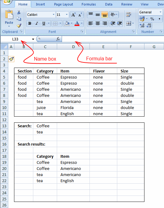
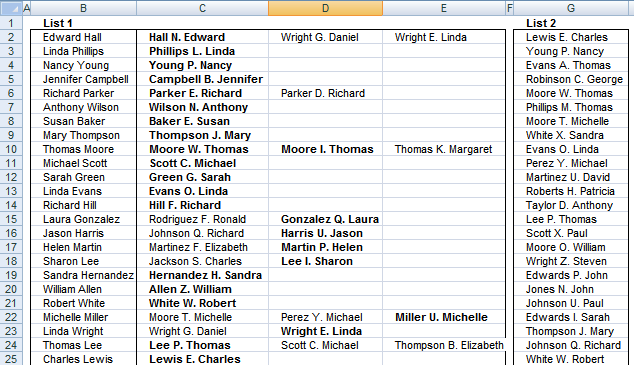
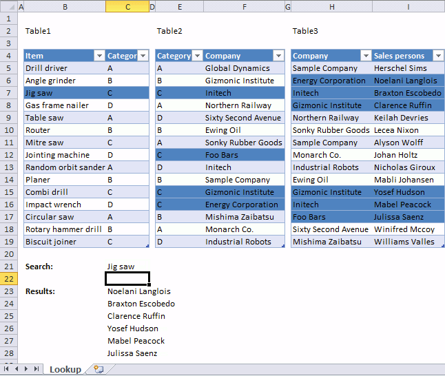
I will start with the picture of results and then give the formulas. For me, Table1 is on the left, Table2 on the right.

Formulas
The formulas are very similar, the main difference is which column to return in the IF part which generates the array for INDEX. The conditional part of the IF is the same for all columns. Note that using Tables here really helps copying around the formulas since the ranges cannot change under us.
These are all array formulas and need to be entered with CTRL+SHIFT+ENTER.
Table2[Item]
=INDEX(IF(Table1[Re-Order Qty]>Table1[On-hand Qty],Table1[Item],"N/A"), MATCH([@Seq],Table1[Seq],0))
Table2[Re-Order Qty]
=INDEX(IF(Table1[Re-Order Qty]>Table1[On-hand Qty],Table1[Re-Order Qty],"N/A"), MATCH([@Seq],Table1[Seq],0))
Table2[On-hand Qty]
=INDEX(IF(Table1[Re-Order Qty]>Table1[On-hand Qty],Table1[On-hand Qty],"N/A"), MATCH([@Seq],Table1[Seq],0))
The main idea behind these formulas is:
- Return a new array based on the conditional. This new array will return the desired column (
Item,Re-order, …) or it will returnN/Aif the conditional isFALSE. This requires the array formula entry since it is going row by row in theIF. - The
MATCHpart of the formula to get the row number is «standard». We are simply looking for theSeqnumber inTable1. This determines which row of the newarrayto return.
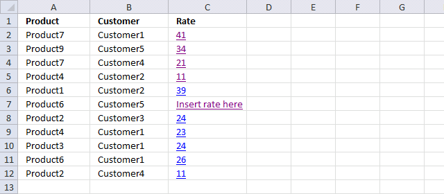
I’m trying to find a formula that will allow me to display multiple fields of data when a specific value (a product SKU) is entered into a cell.
I managed to get this to work with a VLOOKUP formula, whereby I could enter the SKU into one cell, and have the following cells display various values, such as the brand, item, Net cost, VAT, gross price and so on.
However, want to use an INDEX formula instead so that if I edit the reference table then it won’t affect the returned results. I also want to be able to specify which columns/value are returned (for example, I don’t necessarily want to display the Net cost of a product.
From what I can tell, VLOOKUP only allows for either a single column’s value to be returned, or all of the specified columns from left to right, with no option to omit any.
I think I need a combination of IF and INDEX, whereby IF the value matches an SKU in, say, Column A, then values relating to that product code are returned.
I thought I was getting there with the following formula (albeit only being able to return one value):
=IF((P15=D:D),INDEX($E$15:$O$105,0,2)).
D is the worksheet column in which all of the SKUs are listed.
This worked if I entered the relevant SKU on row 15, as it returned the correct gross price that was displayed in column 2 of the reference table.
However, a value is only returned if the SKU is that of row 15, otherwise it displays ‘FALSE’ if I try and search prices using any other any other SKU input.
This has been driving me mad for hours, so I’d be hugely grateful if anyone is able to enlighten me.
Thank you.
This post will guide you how to use Excel INDEX function with syntax and examples in Microsoft excel.
Table of Contents
- Description
- Syntax
- Excel INDEX Function Example
- More Excel INDEX Formula Examples
Description
The Excel INDEX function returns a value from a table based on the index (row number and column number). You can use INDEX function to extract entire rows or entire columns. This function is used to combine with the MATCH function to lookup value in a range or array.
The INDEX function is a build-in function in Microsoft Excel and it is categorized as a Lookup and Reference Function.
The INDEX function is available in Excel 2016, Excel 2013, Excel 2010, Excel 2007, Excel 2003, Excel XP, Excel 2000, Excel 2011 for Mac.
Syntax
There are two ways to use the INDEX function in excel:
If you want to get the value of a specified cell or array of cell, you can refer to Array form.
If you want to get a reference to specified cells, you can refer to Reference form.
The syntax of the INDEX function is as below:
= INDEX (array, row_num,[column_num])      #Array form
=INDEX(reference, row_num,[column_num],[area_num)     #Reference form
The array form is used in most cases, and if the first argument of the INDEX function is an array constant, you need to use the array form. If you want to perform a three-way lookup in a range, you can use the reference form.
Where the INDEX function arguments are:
- array -This is a required argument. A range of cells or data array. If array contains only one row or column, the corresponding row_num or Column_num argument is optional.
- Row_num – The row number in data array. If Row_num is omitted, column_num is required.
- Column_num – The column position in data array. If Column_num is omitted, row_num is required.
- Area_num – it is set as a number. If the first argument point to more cell ranges, if area_num is set to 1, then the first area will be selected.
Note:
- If you set the row_num and column_num at the same time, the INDEX function will return the value in the cell at the intersection of row number and column number.
- If you set the value of row_num or column_num to 0, the INDEX function will return the array of values for the entire row or column in the array data.
- Row_num and Column_num must point to a cell within array data, if not, the index function returns #REF!
Excel INDEX Function Example
The below examples will show you how to use Excel INDEX Lookup and Reference Function to return a value from a table based on the intersection of row number and column number.
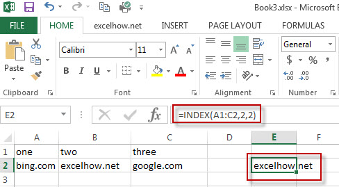
#1 To get the value at the intersection of the second row and second column in the table array: A1:C2, just using the following excel formula:
=INDEX(A1:C2,2,1)
#2 use reference form to extract a value form the second area of C2:D5. Using the following formula.
=INDEX((B1:C5,C2:D5),2,2,2)
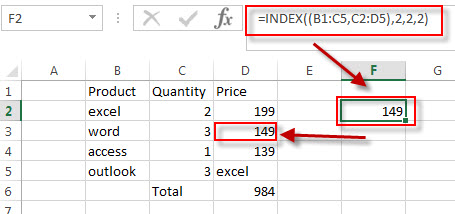
You will see that the intersection of the second row and second column in the second area of C2:D5, which is the contents of cell D3. It returns 149.
More Excel INDEX Formula Examples
- Get the First Match in Two Excel Ranges
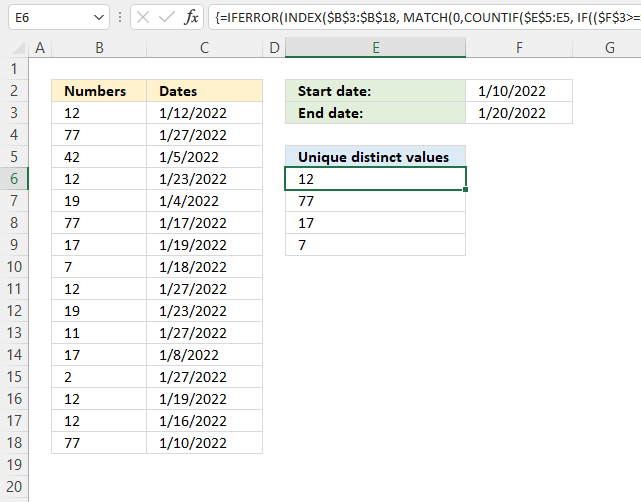
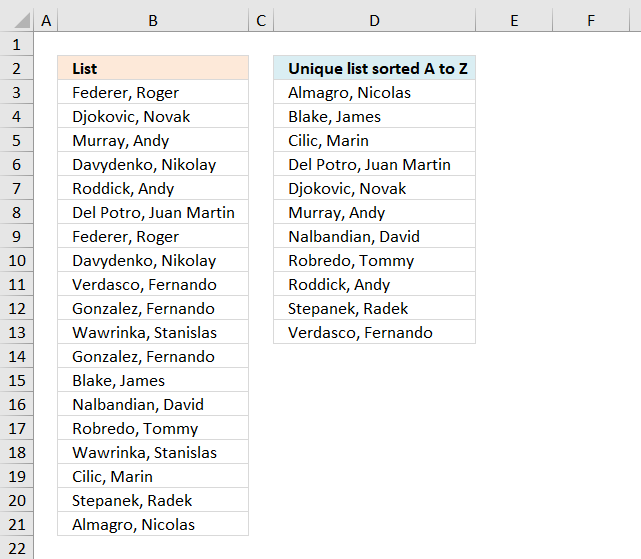
If you want to find the first match between two excel ranges, you can use a combination of the INDEX function, the MATCH function and COUNTIF function to create a new formula…. - Extract a List of Unique Values from a Column Range
f you want to extract a list of unique items from a column or range, you can use a combination of the IFERROR function, the INDEX function, the MATCH function and the COUNTIF function to create an array formula….. - Find the Relative Position in a Range or Table
If you want to know the relative row position for all rows in an Excel Range (B3:D6), you can use a excel Array formula as follows:=ROW(B3:D6)- ROW(B3) + 1. You can also use another excel array formula to get the same result as follows:=ROW(B3:D6)-ROW(INDEX(B3:D6,1,1))+1… - Get the Last Row Number in a Range
If you want to get the last row number in a range, you need to know the first row number and the total rows number of a range, then perform the addition operation, then subtract 1, the last result is the last row number for that range.… - Get the First Row Number in a Range
If the ROW function use a Range as its argument, it only returns the first row number.You can also use the ROW function within the MIN function to get the first row number in a range. You can also use the INDEX function to get the reference of the first row in a range, then combined to the ROW function to get the first row number of a range.… - Get the position of Last Occurrence of a value in a column
If you want to find the position number of the last occurrence of a specific value in a column (a single range), you can use an array formula with a combination of the MAX function, IF function, ROW function and INDEX Function. - Lookup the Next Largest Value
If you want to get the next largest value in another column, you can use a combination of the INDEX function and the MATCH function to create an excel formula. You can use the following formula:=INDEX(A2:A5,MATCH(200,A2:A5)+1)… - Reverse a List or Range
If you want to reverse a list or range, you can use a combination of the INDEX function, the COUNTA function, the ROW function or ROWS function to create a new formula. you can use the following formula:=INDEX($A$2:$A$5,COUNTA($A$2:$A$5)-ROWS($C$2:C2)+1)… - Lookup the Value with Multiple Criteria
If you want to lookup the value with multiple criteria in a range, you can use a combination with the INDEX function and MATCH function to create an array formula… - Transpose Values Based on the Multiple Lookup Criteria
If you want to lookup the value with multiple criteria, and then transpose the last results, you can use the INDEX function with the MATCH function to create a new formula.… - Get nth Match with One Criteria using INDEX/MATCH
if you want to find the 2th occurrence of the member “jenny” in the range B2:B10 and extracts its relative bonus value in the range D2:D10, you can used the following array formula:=INDEX(D2:D10, SMALL(IF(B2:B10=”jenny”, ROW(B2:B10)-ROW(INDEX(B2:B10,1,1))+1),2))… - Find the nth Largest Value
To get the 1st, 2nd, 3rd, or nth largest value in a range (single column, or row), you can use the LARGE function… - Find the nth Smallest Value
You can use the SMALL function to get the 1st, 2nd, 3rd, or nth smallest value in an array or range. Also you can use the SMALL function within the INDEX function to extract the relative value of the same row… - Extract the Entire Column of a Matched Value
If you want to lookup value in a range and then retrieve the entire row, you can use a combination of the INDEX function and the MATCH function to create a new excel formula..… - Lookup Entire Row using INDEX/MATCH
If you want to lookup entire row and then return all values of the matched row, you can use a combination of the INDEX function and the MATCH function to create a new excel array formula. - Find nth Occurrence with Multiple Criteria Using INDEX/MATCH
If you want to find the nth occurrence with multiple criteria, you can use a combination with the INDEX function, SMALL function, nested IF function and ROW function to create a complex excel formula like this:=INDEX(Array,SMALL(IF(Range1… - Two-way Lookup Formula
If you want to look up a value in a table using both rows and columns, you can use a combination with the INDEX function and the MATCH function to create an excel formula.… - SUM a Column with Lookup value in a Range
If you want to lookup value in a range and then retrieve the entire row, you can use the MATCH function within the INDEX function… - Get Cell Address of a Lookup Value
If you want to lookup a value in a range or column and return the cell address of the first match of lookup value, you can use a combination with the CELL function, the INDEX function and the MATCH function…. - Transpose Multiple Columns into One Column
You can use the following excel formula to transpose multiple columns that contain a range of data into a single column, and you can also write an Excel VBA Macro to transpose the data of range in B1:D4 into single column F quickly… - Flip a Column of Data Vertically
How do I remove time part from a date in Excel. How to get only date part from the date with time values via Format cells feature or Excel function. How to extract date from a date and time with VBA code in Excel…. - Finding the Max and Min value in an Alphanumeric Data
if you want to find the Maximal or minimal string value from an alphanumeric data list in the range B1:B5, you can create a formula based on the LOOKUP function and the COUNTIF function.…. - Sum Specific Row or Column in Named Range
Assuming that you have a name range “excelhow”, if you want to sum a specific row (row 2) in named range, you need to create a formula based on the SUM function and the OFFSET function and the COLUMNS function to achieve the reuslt…. - Randomly Select Cells
If you want to randomly select cells from a range of cells, you can use a formula based on the INDEX function, the RANDBETWEEN function and the Rows function….. - List all Worksheet Names
Assuming that you have a workbook that has hundreds of worksheets and you want to get a list of all the worksheet names in the current workbook. And the below will introduce 3 methods with you..… - Split Data in One Column to Multiple Columns
If you want to split each sets in one column from row to row in stacked columns, and you need to create a formula based on the OFFSET function, the COLUMNS function, and the ROWS function..… - VLOOKUP Return Multiple Values Horizontally
You can create a complex array formula based on the INDEX function, the SMALL function, the IF function, the ROW function and the COLUMN function to vlookup a value and then return multiple corresponding values horizontally in Excel.… - Copy and Paste Only Non-blank Cells
If you want only copy non-blank cells in a range in Excel, you need to select the non-blank cells firstly, then press Ctrl +C keys to copy the selected cells. So how to only select all non-blank cells in the selected range in your worksheet..… - Generate All Possible Combinations of Two Lists
You can use a formula based on the IF function, the ROW function, the COUNTA function, The INDEX function and the MOD function to get a list of all possible combinations from those two list…. - Find Closest Value or Nearest Value in a Range
You need to use an excel array formula based on the INDEX function, the MATCH function, the MIN function and the ABS function to find Closest Value or Nearest Value in a Range in Excel…
This article explains in simple terms how to use INDEX and MATCH together to perform lookups. It takes a step-by-step approach, first explaining INDEX, then MATCH, then showing you how to combine the two functions together to create a dynamic two-way lookup. There are more advanced examples further down the page.
INDEX function | MATCH function | INDEX and MATCH | 2-way lookup | Left lookup | Case-sensitive | Closest match | Multiple criteria | More examples
The INDEX Function
The INDEX function in Excel is fantastically flexible and powerful, and you’ll find it in a huge number of Excel formulas, especially advanced formulas. But what does INDEX actually do? In a nutshell, INDEX retrieves the value at a given location in a range. For example, let’s say you have a table of planets in our solar system (see below), and you want to get the name of the 4th planet, Mars, with a formula. You can use INDEX like this:
=INDEX(B3:B11,4)

INDEX returns the value in the 4th row of the range.
Video: How to look things up with INDEX
What if you want to get the diameter of Mars with INDEX? In that case, we can supply both a row number and a column number, and provide a larger range. The INDEX formula below uses the full range of data in B3:D11, with a row number of 4 and column number of 2:
=INDEX(B3:D11,4,2)

INDEX retrieves the value at row 4, column 2.
To summarize, INDEX gets a value at a given location in a range of cells based on numeric position. When the range is one-dimensional, you only need to supply a row number. When the range is two-dimensional, you’ll need to supply both the row and column number.
At this point, you may be thinking «So what? How often do you actually know the position of something in a spreadsheet?»
Exactly right. We need a way to locate the position of things we’re looking for.
Enter the MATCH function.
The MATCH function
The MATCH function is designed for one purpose: find the position of an item in a range. For example, we can use MATCH to get the position of the word «peach» in this list of fruits like this:
=MATCH("peach",B3:B9,0)

MATCH returns 3, since «Peach» is the 3rd item. MATCH is not case-sensitive.
MATCH doesn’t care if a range is horizontal or vertical, as you can see below:
=MATCH("peach",C4:I4,0)

Same result with a horizontal range, MATCH returns 3.
Video: How to use MATCH for exact matches
Important: The last argument in the MATCH function is match_type. Match_type is important and controls whether matching is exact or approximate. In many cases you will want to use zero (0) to force exact match behavior. Match_type defaults to 1, which means approximate match, so it’s important to provide a value. See the MATCH page for more details.
INDEX and MATCH together
Now that we’ve covered the basics of INDEX and MATCH, how do we combine the two functions in a single formula? Consider the data below, a table showing a list of salespeople and monthly sales numbers for three months: January, February, and March.

Let’s say we want to write a formula that returns the sales number for February for a given salesperson. From the discussion above, we know we can give INDEX a row and column number to retrieve a value. For example, to return the February sales number for Frantz, we provide the range C3:E11 with a row 5 and column 2:
=INDEX(C3:E11,5,2) // returns $5194
But we obviously don’t want to hardcode numbers. Instead, we want a dynamic lookup.
How will we do that? The MATCH function of course. MATCH will work perfectly for finding the positions we need. Working one step at a time, let’s leave the column hardcoded as 2 and make the row number dynamic. Here’s the revised formula, with the MATCH function nested inside INDEX in place of 5:
=INDEX(C3:E11,MATCH("Frantz",B3:B11,0),2)
Taking things one step further, we’ll use the value from H2 in MATCH:
=INDEX(C3:E11,MATCH(H2,B3:B11,0),2)

MATCH finds «Frantz» and returns 5 to INDEX for row.
To summarize:
- INDEX needs numeric positions.
- MATCH finds those positions.
- MATCH is nested inside INDEX.
Let’s now tackle the column number.
Two-way lookup with INDEX and MATCH
Above, we used the MATCH function to find the row number dynamically, but hardcoded the column number. How can we make the formula fully dynamic, so we can return sales for any given salesperson in any given month? The trick is to use MATCH twice – once to get a row position, and once to get a column position.
From the examples above, we know MATCH works fine with both horizontal and vertical arrays. That means we can easily find the position of a given month with MATCH. For example, this formula returns the position of March, which is 3:
=MATCH("Mar",C2:E2,0) // returns 3
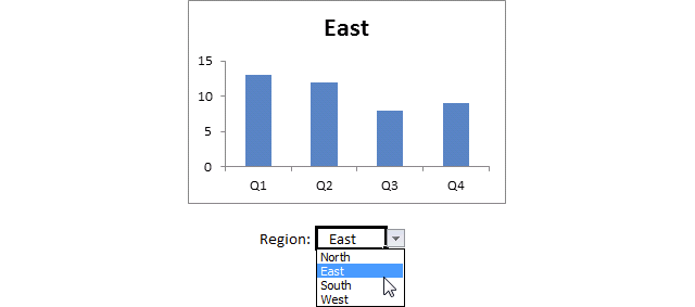
But of course we don’t want to hardcode any values, so let’s update the worksheet to allow the input of a month name, and use MATCH to find the column number we need. The screen below shows the result:

A fully dynamic, two-way lookup with INDEX and MATCH.
=INDEX(C3:E11,MATCH(H2,B3:B11,0),MATCH(H3,C2:E2,0))
The first MATCH formula returns 5 to INDEX as the row number, the second MATCH formula returns 3 to INDEX as the column number. Once MATCH runs, the formula simplifies to:
=INDEX(C3:E11,5,3)
and INDEX correctly returns $10,525, the sales number for Frantz in March.
Note: you could use Data Validation to create dropdown menus to select salesperson and month.
Video: How to do a two-way lookup with INDEX and MATCH
Video: How to debug a formula with F9 (to see MATCH return values)
Left lookup
One of the key advantages of INDEX and MATCH over the VLOOKUP function is the ability to perform a «left lookup». Simply put, this just means a lookup where the ID column is to the right of the values you want to retrieve, as seen in the example below:

Read a detailed explanation here.
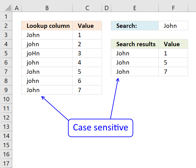
Case-sensitive lookup
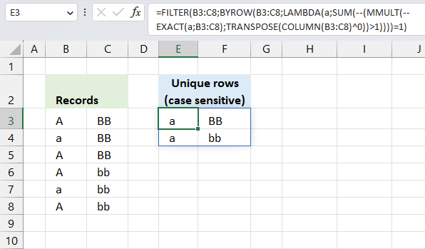
By itself, the MATCH function is not case-sensitive. However, you use the EXACT function with INDEX and MATCH to perform a lookup that respects upper and lower case, as shown below:

Read a detailed explanation here.
Note: this is an array formula and must be entered with control + shift + enter, except in Excel 365.
Closest match
Another example that shows off the flexibility of INDEX and MATCH is the problem of finding the closest match. In the example below, we use the MIN function together with the ABS function to create a lookup value and a lookup array inside the MATCH function. Essentially, we use MATCH to find the smallest difference. Then we use INDEX to retrieve the associated trip from column B.

Read a detailed explanation here.
Note: this is an array formula and must be entered with control + shift + enter, except in Excel 365.
Multiple criteria lookup
One of the trickiest problems in Excel is a lookup based on multiple criteria. In other words, a lookup that matches on more than one column at the same time. In the example below, we are using INDEX and MATCH and boolean logic to match on 3 columns: Item, Color, and Size:

Read a detailed explanation here. You can use this same approach with XLOOKUP.
Note: this is an array formula and must be entered with control + shift + enter, except in Excel 365.
More examples of INDEX + MATCH
Here are some more basic examples of INDEX and MATCH in action, each with a detailed explanation:
- Basic INDEX and MATCH exact (features Toy Story)
- Basic INDEX and MATCH approximate (grades)
- Two-way lookup with INDEX and MATCH (approximate match)
Функция INDEX (ИНДЕКС) в Excel используется для получения данных из таблицы, при условии что вы знаете номер строки и столбца, в котором эти данные находятся.
Например, в таблице ниже, вы можете использовать эту функцию для того, чтобы получить результаты экзамена по Физике у Андрея, зная номер строки и столбца, в которых эти данные находятся.

Содержание
- Что возвращает функция
- Синтаксис
- Аргументы функции
- Дополнительная информация
- Примеры использования функции ИНДЕКС в Excel
- Пример 1. Ищем результаты экзамена по физике для Алексея
- Пример 2. Создаем динамический поиск значений с использованием функций ИНДЕКС и ПОИСКПОЗ
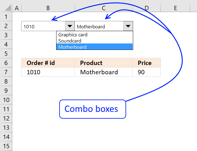
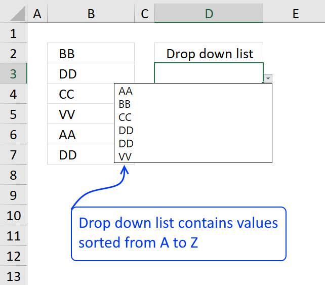
- Пример 3. Создаем динамический поиск значений с использованием функций INDEX (ИНДЕКС) и MATCH (ПОИСКПОЗ) и выпадающего списка
- Пример 4. Использование трехстороннего поиска с помощью INDEX (ИНДЕКС) / MATCH (ПОИСКПОЗ)
Что возвращает функция
Возвращает данные из конкретной строки и столбца табличных данных.
Синтаксис
=INDEX (array, row_num, [col_num]) — английская версия
=INDEX (array, row_num, [col_num], [area_num]) — английская версия
=ИНДЕКС(массив; номер_строки; [номер_столбца]) — русская версия
=ИНДЕКС(ссылка; номер_строки; [номер_столбца]; [номер_области]) — русская версия
Аргументы функции
- array (массив) — диапазон ячеек или массив данных для поиска;
- row_num (номер_строки) — номер строки, в которой находятся искомые данные;
- [col_num] ([номер_столбца]) (необязательный аргумент) — номер колонки, в которой находятся искомые данные. Этот аргумент необязательный. Но если в аргументах функции не указаны критерии для row_num (номер_строки), необходимо указать аргумент col_num (номер_столбца);
- [area_num] ([номер_области]) — (необязательный аргумент) — если аргумент массива состоит из нескольких диапазонов, то это число будет использоваться для выбора всех диапазонов.
Дополнительная информация
- Если номер строки или колонки равен “0”, то функция возвращает данные всей строки или колонки;
- Если функция используется перед ссылкой на ячейку (например, A1), она возвращает ссылку на ячейку вместо значения (см. примеры ниже);
- Чаще всего INDEX (ИНДЕКС) используется совместно с функцией MATCH (ПОИСКПОЗ);
- В отличие от функции VLOOKUP (ВПР), функция INDEX (ИНДЕКС) может возвращать данные как справа от искомого значения, так и слева;
- Функция используется в двух формах — Массива данных и Формы ссылки на данные:
— Форма «Массива» используется когда вы хотите найти значения, основанные на конкретных номерах строк и столбцов таблицы;
— Форма «Ссылок на данные» используется при поиске значений в нескольких таблицах (используете аргумент [area_num] ([номер_области]) для выбора таблицы и только потом сориентируете функцию по номеру строки и столбца.
Примеры использования функции ИНДЕКС в Excel
Пример 1. Ищем результаты экзамена по физике для Алексея
Предположим, у вас есть результаты экзаменов в табличном виде по нескольким студентам:
Для того, чтобы найти результаты экзамена по физике для Андрея нам нужна формула:
=INDEX($B$3:$E$9,3,2) — английская версия
=ИНДЕКС($B$3:$E$9;3;2) — русская версия
В формуле мы определили аргумент диапазона данных, где мы будем искать данные $B$3:$E$9. Затем, указали номер строки “3”, в которой находятся результаты экзамена для Андрея, и номер колонки “2”, где находятся результаты экзамена именно по физике.
Пример 2. Создаем динамический поиск значений с использованием функций ИНДЕКС и ПОИСКПОЗ
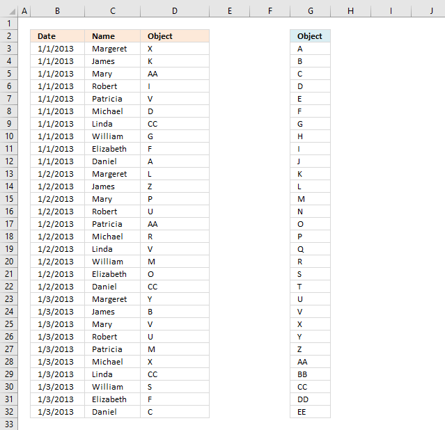
Не всегда есть возможность указать номера строки и столбца вручную. У вас может быть огромная таблица данных, отображение данных которой вы можете сделать динамическим, чтобы функция автоматически идентифицировала имя или экзамен, указанные в ячейках, и дала правильный результат.
Пример динамического отображения данных ниже:

Для динамического отображения данных мы используем комбинацию функций INDEX (ИНДЕКС) и MATCH (ПОИСКПОЗ).
Вот такая формула поможет нам добиться результата:
=INDEX($B$3:$E$9,MATCH($G$4,$A$3:$A$9,0),MATCH($H$3,$B$2:$E$2,0)) — английская версия
=ИНДЕКС($B$3:$E$9;ПОИСКПОЗ($G$4;$A$3:$A$9;0);ПОИСКПОЗ($H$3;$B$2:$E$2;0)) — русская версия
В формуле выше, не используя сложного программирования, мы с помощью функции MATCH (ПОИСКПОЗ) сделали отображение данных динамическим.
Динамический отображение строки задается следующей частью формулы —
MATCH($G$4,$A$3:$A$9,0) — английская версия
ПОИСКПОЗ($G$4;$A$3:$A$9;0) — русская версия
Она сканирует имена студентов и определяет значение поиска ($G$4 в нашем случае). Затем она возвращает номер строки для поиска в наборе данных. Например, если значение поиска равно Алексей, функция вернет “1”, если это Максим, оно вернет “4” и так далее.
Динамическое отображение данных столбца задается следующей частью формулы —
MATCH($H$3,$B$2:$E$2,0) — английская версия
ПОИСКПОЗ($H$3;$B$2:$E$2;0) — русская версия
Она сканирует имена объектов и определяет значение поиска ($H$3 в нашем случае). Затем она возвращает номер столбца для поиска в наборе данных. Например, если значение поиска Математика, функция вернет “1”, если это Физика, функция вернет “2” и так далее.
Больше лайфхаков в нашем Telegram Подписаться
Пример 3. Создаем динамический поиск значений с использованием функций INDEX (ИНДЕКС) и MATCH (ПОИСКПОЗ) и выпадающего списка
На примере выше мы вручную вводили имена студентов и названия предметов. Вы можете сэкономить время на вводе данных, используя выпадающие списки. Это актуально, когда количество данных огромное.
Используя выпадающие списки, вам нужно просто выбрать из списка имя студента и функция автоматически найдет и подставит необходимые данные.
Пример ниже:

Используя такой подход, вы можете создать удобный дашборд, например для учителя. Ему не придется заниматься фильтрацией данных или прокруткой листа со студентами, для того чтобы найти результаты экзамена конкретного студента, достаточно просто выбрать имя и результаты динамически отразятся в лаконичной и удобной форме.
Для того, чтобы осуществить динамическую подстановку данных с использованием функций INDEX (ИНДЕКС) и MATCH (ПОИСКПОЗ) и выпадающего списка, мы используем ту же формулу, что в Примере 2:
=INDEX($B$3:$E$9,MATCH($G$4,$A$3:$A$9,0),MATCH($H$3,$B$2:$E$2,0)) — английская версия
=ИНДЕКС($B$3:$E$9;ПОИСКПОЗ($G$4;$A$3:$A$9;0);ПОИСКПОЗ($H$3;$B$2:$E$2;0)) — русская версия
Единственное отличие, от Примера 2, мы на месте ввода имени и предмета создадим выпадающие списки:
- Выбираем ячейку, в которой мы хотим отобразить выпадающий список с именами студентов;
- Кликаем на вкладку “Data” => Data Tools => Data Validation;
- В окне Data Validation на вкладке “Settings” в подразделе Allow выбираем “List”;
- В качестве Source нам нужно выбрать диапазон ячеек, в котором указаны имена студентов;
- Кликаем ОК
Теперь у вас есть выпадающий список с именами студентов в ячейке G5. Таким же образом вы можете создать выпадающий список с предметами.
Пример 4. Использование трехстороннего поиска с помощью INDEX (ИНДЕКС) / MATCH (ПОИСКПОЗ)
Функция INDEX (ИНДЕКС) может быть использована для обработки трехсторонних запросов.
Что такое трехсторонний поиск?
В приведенных выше примерах мы использовали одну таблицу с оценками для студентов по разным предметам. Это пример двунаправленного поиска, поскольку мы используем две переменные для получения оценки (имя студента и предмет).
Теперь предположим, что к концу года студент прошел три уровня экзаменов: «Вступительный», «Полугодовой» и «Итоговый экзамен».
Трехсторонний поиск — это возможность получить отметки студента по заданному предмету с указанным уровнем экзамена.
Вот пример трехстороннего поиска:
В приведенном выше примере, кроме выбора имени студента и названия предмета, вы также можете выбрать уровень экзамена. Основываясь на уровне экзамена, формула возвращает соответствующее значение из одной из трех таблиц.
Для таких расчетов нам поможет формула:
=INDEX(($B$3:$E$7,$B$11:$E$15,$B$19:$E$23),MATCH($G$4,$A$3:$A$7,0),MATCH($H$3,$B$2:$E$2,0),IF($H$2=»Вступительный»,1,IF($H$2=»Полугодовой»,2,3))) — английская версия
=ИНДЕКС(($B$3:$E$7;$B$11:$E$15;$B$19:$E$23);ПОИСКПОЗ($G$4;$A$3:$A$7;0);ПОИСКПОЗ($H$3;$B$2:$E$2;0); ЕСЛИ($H$2=»Вступительный»;1;ЕСЛИ($H$2=»Полугодовой»;2;3))) — русская версия
Давайте разберем эту формулу, чтобы понять, как она работает.
Эта формула принимает четыре аргумента. Функция INDEX (ИНДЕКС) — одна из тех функций в Excel, которая имеет более одного синтаксиса.
=INDEX (array, row_num, [col_num]) — английская версия
=INDEX (array, row_num, [col_num], [area_num]) — английская версия
=ИНДЕКС(массив; номер_строки; [номер_столбца]) — русская версия
=ИНДЕКС(ссылка; номер_строки; [номер_столбца]; [номер_области]) — русская версия
По всем вышеприведенным примерам мы использовали первый синтаксис, но для трехстороннего поиска нам нужно использовать второй синтаксис.
Рассмотрим каждую часть формулы на основе второго синтаксиса.
- array (массив) – ($B$3:$E$7,$B$11:$E$15,$B$19:$E$23):Вместо использования одного массива, в данном случае мы использовали три массива в круглых скобках.
- row_num (номер_строки) – MATCH($G$4,$A$3:$A$7,0): функция MATCH (ПОИСКПОЗ) используется для поиска имени студента для ячейки $G$4 из списка всех студентов.
- col_num (номер_столбца) – MATCH($H$3,$B$2:$E$2,0): функция MATCH (ПОИСКПОЗ) используется для поиска названия предмета для ячейки $H$3 из списка всех предметов.
- [area_num] ([номер_области]) – IF($H$2=”Вступительный”,1,IF($H$2=”Полугодовой”,2,3)): Значение номера области сообщает функции INDEX (ИНДЕКС), какой массив с данными выбрать. В этом примере у нас есть три массива в первом аргументе. Если вы выберете «Вступительный» из раскрывающегося меню, функция IF (ЕСЛИ) вернет значение “1”, а функция INDEX (ИНДЕКС) выберут 1-й массив из трех массивов ($B$3:$E$7).
Уверен, что теперь вы подробно изучили работу функции INDEX (ИНДЕКС) в Excel!
In this tutorial, we’ll dive into the powerful Excel INDEX and MATCH functions, which are essential for manipulating and analyzing large sets of data.
We’ll start by exploring what these functions do and how they retrieve specific information from a table, and then we’ll write INDEX and MATCH formulas together as an alternative to the VLOOKUP formula. We’ll also cover some practical use cases for INDEX and MATCH formulas.
Note: if you have Excel 2021 or later, or Microsoft 365 you should use the XLOOKUP function as this is easier and potentially more efficient.
Watch the INDEX and MATCH Video

Download the Excel File
Enter your email address below to download the sample workbook.
By submitting your email address you agree that we can email you our Excel newsletter.
How the INDEX function works:
The INDEX function returns the value at the intersection of a column and a row.
The syntax for the INDEX function is:
=INDEX(reference, row_num,[column_num], [area_num])
In English:
=INDEX( the range of your table, the row number of the table that your data is in, the column number of the table that your data is in, and if your reference specifies two or more ranges (areas) then specify which area*)
*Typically only one area is specified so the area_num argument can be omitted. The examples below don’t require area_num.
INDEX will return the value that is in the cell at the intersection of the row and column you specify.
For example, looking at the table below in the range B17:F24 we can use INDEX to return the number of program views for Bat Man in the North region with a formula as follows:
=INDEX(B17:F24,2,3)
The result returned is 91.

On its own the INDEX function is pretty inflexible because you have to hard key the row and column number, and that’s why it works better with the MATCH function.
Note: You may have noticed that the INDEX function works in a similar way to the OFFSET function, in fact you can often interchange them and achieve the same results.
How the MATCH function works:
The MATCH function finds the position of a value in a list. The list can either be in a row or a column.
The syntax for the MATCH function is:
=MATCH(lookup_value, lookup_array, [match_type])
Now I don’t want to go all syntaxy (real word 🙂 ) on you, but I’d like to point out some important features of the [match_type] argument:
- The match_type argument specifies how Excel matches the lookup_value with values in lookup_array. You can choose from -1, 0 or 1 (1 is the default)
- [match_type] is an optional argument, hence the square brackets. If you leave it out Excel will use the default of 1, which means it will find the largest value that is <= to the lookup_value. The values in the lookup_array must be in ascending order when using 1 or omitting this argument..
- 0 will find the first value that is exactly equal to the lookup_value. The values in the lookup_array can be in any order.
- -1 finds the smallest value that is >= to the lookup_value. The values in the lookup_array must be in descending order, for example: TRUE, FALSE, Z-A, …2, 1, 0, -1, -2, …, and so on.
Ok, that’s enough of the syntax.
In English and using the previous example:
=MATCH(find what row Bat Man is on, in the column range B17:B24, match it exactly (for this we'll use 0 as our argument))
The result is row 2.
We can also use MATCH to find the column number like this:
=MATCH(find what column North is in, in the row range B17:F17, match it exactly (again we'll use 0 as our argument))
The result is column 3.
So in summary, the INDEX function returns the value in the cell you specify, and the MATCH function tells you the column or row number for the value you are looking up.
INDEX MATCH Together:
The INDEX and MATCH functions are a popular alternative to the VLOOKUP. Even though I still prefer VLOOKUP as it’s more straight forward to use, there are certain things the INDEX + MATCH functions can do that VLOOKUP can’t. More on that later.
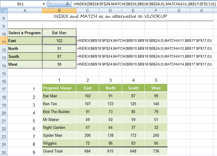
Using the above example data we’ll use the INDEX and MATCH functions to find the program views for Bat Man in the East region.
=INDEX( the range of your table, replace this with a MATCH function to find the row number for Bat Man, replace this with a MATCH function to find the column number for East)
The formula will read like this:
=INDEX( return the value in the table range B17:F24 in the cell that is at the intersection of, MATCH( the row Bat Man is on) and, MATCH(the column East is in)
The formula looks like this:
=INDEX($B$18:$F$24,MATCH("Bat Man",$B$18:$B$24,0), MATCH(“East”,$B$17:$F$17,0))
So why would you put yourself through all that rigmarole when VLOOKUP can do the same job.
Reasons to use INDEX and MATCH rather than VLOOKUP
1) VLOOKUP can’t go left
Taking the table below, let’s say you wanted to find out what program was on the Krafty Kids channel.

VLOOKUP can’t do this because you’d be asking it to find Krafty Kids and then return the value in column B to the left, and VLOOKUP can only look to the right.
In comes INDEX and MATCH with a formula like this:
=INDEX($B$33:$B$40,MATCH("Krafty Kids",$C$33:$C$40,0))
And you get the answer; ‘Mr Maker’.
Notice only the Programs column (B) was referenced in INDEX’s array argument? This means we can omit INDEX’s column number argument as there’s only one column in the INDEX array.
2) Two way lookup
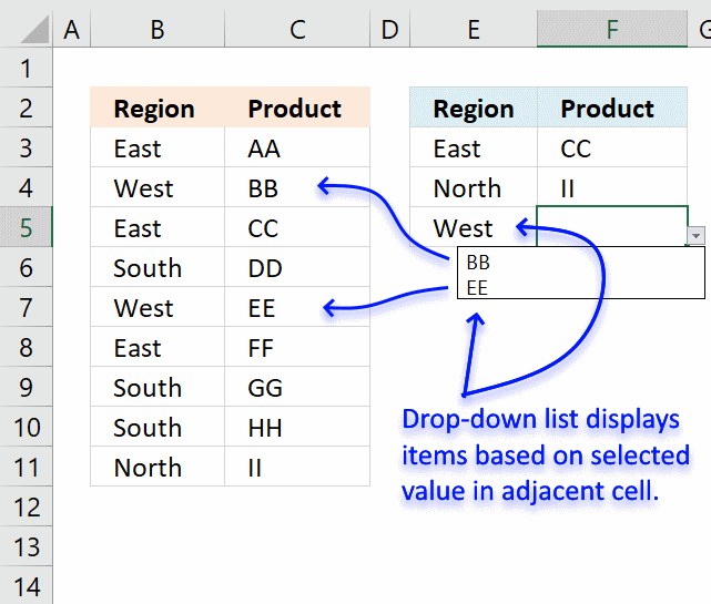
The table below has a drop down list in B1 that enables me to choose the Sales Person from the table, and a drop down list in A2 for the region. In B2 I’ve got an INDEX + MATCH formula that returns the sales that match my two criteria.
=INDEX(A4:J10,MATCH(A2,A4:A10,0),MATCH(B1,A4:J4,0))

Note: An alternative is to use a VLOOKUP and replace the hard keyed column number with a MATCH formula like this:
=VLOOKUP(A2,$A$4:$J$10,MATCH(B1,A4:J4,0),FALSE)
Ways to improve these formulas:
1) Use named ranges instead of $C$33:$C$40 etc. to make formulas more intuitive and quicker to create.
2) An alternative to using a named range is to convert the data to an Excel Table whereby Excel automatically gives the table a named range.
3) If there is nothing else in the columns other than your table you could use column references like this C:C which will search the whole column.
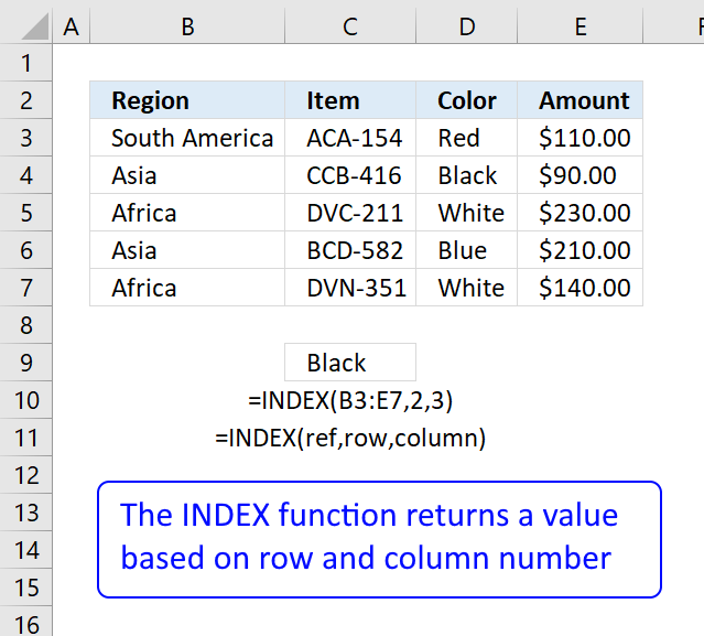
The INDEX function returns a value from a cell range, you specify which value based on a row and column number.
Formula in cell C9:
=INDEX(B3:E7,2,3)
This formula returns a value from row 2 and column 3 based on cell range B3:E7, note these are relative positions.

The image above shows the relative row and column numbers, row 2 and column 3 are highlighted. The intersection of those two is the value the INDEX function returns.
Video
Table of Contents
- Function Syntax
- Arguments
- How to use an array in INDEX function
- How to use the row_num argument
- Return an array of values — INDEX function
- How to use the [column_num] argument
- How to use the [area_num] argument — INDEX function
- How to return the entire row using the INDEX function
- How to return a column
- How to return a cell range
- How to build a dynamic cell reference using the INDEX function
- Get Excel file
1. Excel Function Syntax
INDEX(array, [row_num], [column_num], [area_num])
Back to top
2. Arguments
| array or cell reference | Required. The cell range you want to get a value from. You can also use an array. |
| [row_num] | Optional. The relative row number of a specific value you want to get. If omitted the INDEX function returns all values if you enter it as an array formula. Update! The 365 subscription version of Excel returns all values without needing to enter the formulas an array formula. |
| [column_num] | Optional. The relative column number of a specific value you want to get. If omitted the INDEX function returns all values if you enter it as an array formula. Update! The 365 subscription version of Excel returns all values without needing to enter the formulas an array formula. |
| [area_num] | Optional. A number representing the relative position of one of the ranges in the first argument. |
Back to top
3. How to use an array in INDEX function
The first argument in the INDEX function is array or a cell reference to a cell range. What is an array? An array is a range of values hardcoded into the formula.
To demonstrate in greater detail what an array is you can convert an array or a cell reference to a group of constants by selecting the cell reference and then press F9 to convert the cell reference to values, see the animated image above.
When you convert a cell range to constants Excel automatically creates double quotes around text values, however, note that numbers are not changed.
B6:D8 becomes {«Staple»,10,10;»Binder»,20,6;»Pen»,30,1} and each value is separated by a delimiting character. Comma (,) is used to separate columns and semicolon (;) to separate rows.
The English language version of excel uses commas and semicolons, other language versions of excel may use other characters. You can change this in the Regional settings in Windows.
Here is an example of an array used in an INDEX function:
=INDEX({«Staple», 10, 10; «Binder», 20, 6; «Pen», 30, 1}, 3, 1)
The greatest disadvantage of using an array is that you need to edit the formula if you need to change one of the values in the array, contrary to a cell reference.
Here is an example of a cell reference being used in an INDEX function:
=INDEX(B6:D8, 3, 1)
You don’t need to edit this formula if one of the values in cell range B6:D8 is changed, the formula is using the new value automatically.
Remember that relative cell references (B6:D8) changes when you copy the cell and paste to cells below. Absolute cell references ($B$6:$D$8) do not change when the cell is copied to cells below.
Read more about converting cell references or formulas: Replace a formula with its result
Back to top
4. How to use the row_num argument
The second argument in the INDEX function is the row_num. It allows you to choose the row in an array or cell range, from which to return a value.
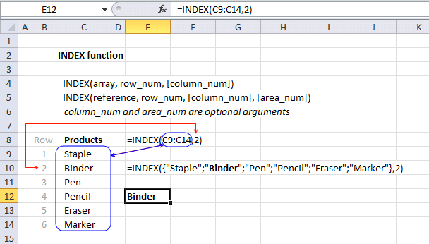
If you use an array or cell range with values distributed in one column only there is no need to use the second optional argument which specifies the column, there is only one column to use. Here is an example of an array containing values in a single column, no comma as a delimiting value in this array which would have indicated that there would have been multiple columns.
=INDEX({«Staple»; «Binder»; «Pen»; «Pencil»; «Eraser»; «Marker»}, 2)
The following formula uses a cell reference instead of hardcoded values:
=INDEX(C9:C14, 2)
Cell range C9:C14 has values separated by a semicolon. The cell range is one-dimensional. In this example, the value from the second row will be returned, see image above.
5. Return an array of values — INDEX function

It is also possible to return an array of values if you omit or use a zero as row_num argument:
=INDEX(C9:C14,)
=INDEX(C9:C14,0)
Both these formulas return an array of values. To be able to display all values you need to enter the formula as an array formula in a cell range that has the same number of cells as the cell range or values in the array.
- Select cell range D3:D8.
- Type the formula =INDEX(C9:C14,0)
- Press and hold CTRL + SHIFT simultaneously.
- Press Enter once.
- Release all keys.
The formula in the formula bar changes to {=INDEX(C9:C14,0)}, do not add these curly brackets yourself, they appear automatically. See the image above.
Update 1/22/2020!

Excel users owning Excel 365 subscription version now have the option to not enter the formula as an array formula but as a regular formula. They are called dynamic arrays and behaves differently than array formulas. Array formulas can still be used in order to be compatible with earlier Excel versions, however, Microsoft suggests that you should from now on use dynamic arrays instead of array formulas.
The formula is entered as a regular formula and extends automatically if the cells needed below are empty, this is called spilling by Microsoft. The remaining cells show a greyed out formula in the formula bar, only the first cell contains a formula in black.
The blue border around the cell range indicates that the cell range contains a spilled formula and disappears when you press with left mouse button on a cell outside the range.
Back to top
6. How to use the [column_num] argument
The column_num argument allows you to choose a column from which to return a value. This argument is optional, for example, if you only have values in a single column.
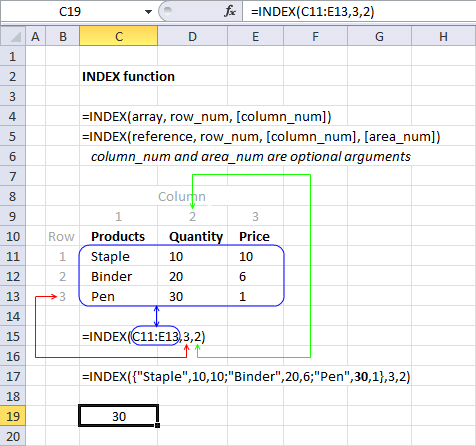
The cell range C11:E13 is two-dimensional meaning there are multiple rows and columns. In this example, the value in the third row and the second column is returned.
=INDEX(C11:E13, 3, 2)
I have greyed out the row and column numbers in the image above, this makes it easier to see that value 30 is where row 3 and column 2 interesects.
The following formula has an array containing constants.
=INDEX({«Staple», 10, 10; «Binder», 20, 6; «Pen», 30, 1}, 3, 2)
{«Staple», 10, 10; «Binder», 20, 6; «Pen», 30, 1} has values separated by commas and semicolons meaning commas separate values between columns and semicolons separate values between rows.
Read more: Looking up data in a cross reference table
Back to top
7. How to use the [area_num] argument — INDEX function
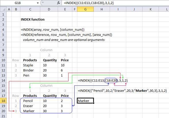
The INDEX function lets you have multiple cell references in the first argument, the area_num argument allows you to pick a cell range in the reference argument.
INDEX(reference, row_num, [column_num], [area_num])
The following formula has two references pointing to two different cell ranges.
=INDEX((C11:E13,C18:E20),3,1,2)
The area_num selects from which cell reference to return a value. In this example, area_num is two therefore the second cell reference is used. The item in the third row and the first column is returned.
Back to top
8. How to return the entire row using the INDEX function
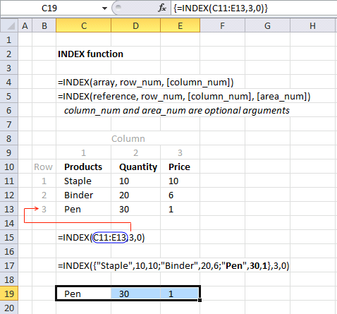
The INDEX function is also capable of returning an array from a column, row, and both columns and rows. The following formula demonstrates how to extract all values from row three:
=INDEX(C11:E13,3,0)
The formula in cell C19:E19 is an array formula.
- Select cell range C19:E19.
- Type =INDEX(C11:E13,3,0) in formula bar.
- Press and hold CTRL + SHIFT simultaeously.
- Press Enter.
- Release all keys.
Back to top
8.1 How to return a column — INDEX function
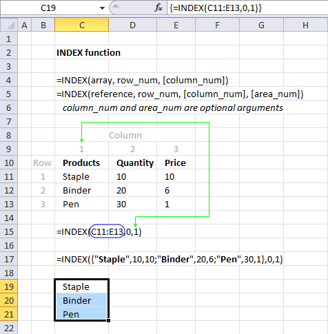
The example above demonstrates an array formula that returns all values from column 1 from cell range C11:E13.
=INDEX(C11:E13, 0, 1)
Back to top
8.2 How to return a two-dimensional cell range — INDEX function
The example below returns all values from a two-dimensional cell range.
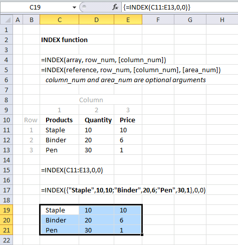
The following array formula returns all values on all rows and columns from a cell range.
=INDEX(C11:E13,0,0)
Back to top
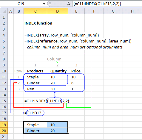
9. How to build a dynamic cell reference using the INDEX function
The INDEX function can also be used to create a cell reference, for example, a dynamic range created by a formula in a named range.
Array formula in cell range C19:D20:
=C11:INDEX(C11:E13,2,2)
INDEX(C11:E13,2,2) returns cell reference D12
C11:D12 returns {«Staple»,10;»Binder»,20}
Back to top
Final note
There are some magic things you can do with the array argument. See this post: No more array formulas?
Back to top
10. Excel file
Back to top
‘INDEX‘ function examples
The following 237 articles contain the INDEX function.


Assign records unique random text strings
This article demonstrates a formula that distributes given text strings randomly across records in any given day meaning they may […]
Auto populate a worksheet
Rodney Schmidt asks: I am a convenience store owner that is looking to make a spreadsheet formula. I want this […]
Basic invoice template
Rattan asks: In my workbook I have three worksheets; «Customer», «Vendor» and «Payment». In the Customer sheet I have a […]
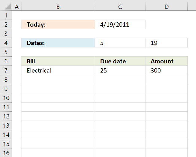
Bill reminder in excel
Brad asks: I’m trying to use your formulas to create my own bill reminder sheet. I envision a workbook where […]
![]()
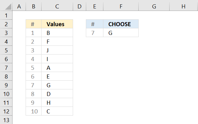
CHOOSE function from list
The picture above shows the CHOOSE function in cell F3, one disadvantage is that you need to press with left […]
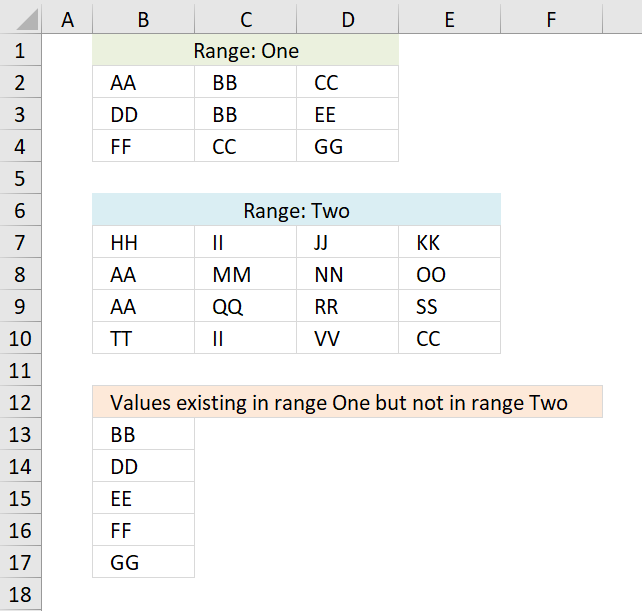
Compare two columns and return differences
This article demonstrates formulas that extract differences between two given lists. The first formula in cell B11 extracts values from […]
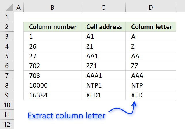
Convert column number to column letter
Use the following formula to convert a column number to a column letter: =LEFT(ADDRESS(1, B3, 4), MATCH(B3, {1; 27; 703})) […]
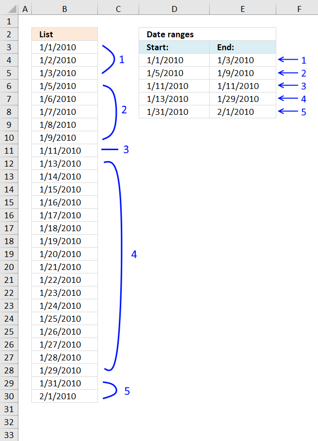
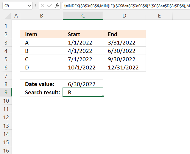
Convert dates into date ranges
The array formula in cell D4 extracts the start dates for date ranges in cell range B3:B30, the array formula […]
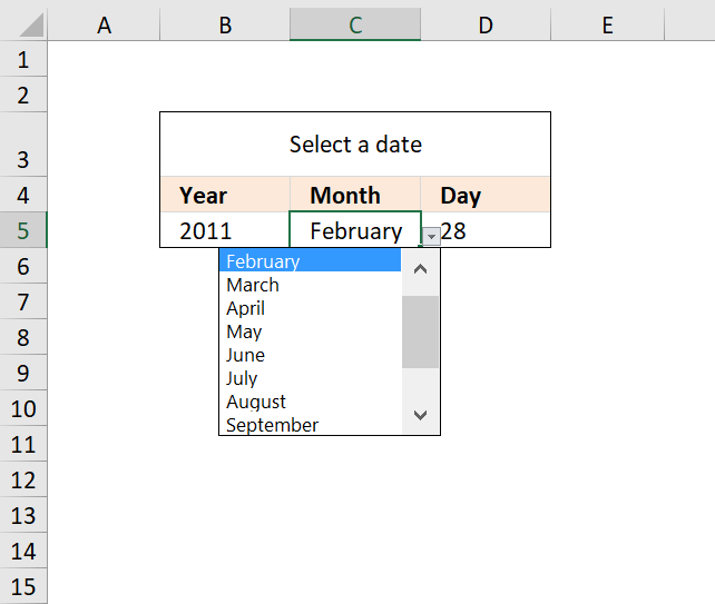
Create a drop down calendar
The drop down calendar in the image above uses a «calculation» sheet and a named range. You can copy the drop-down […]
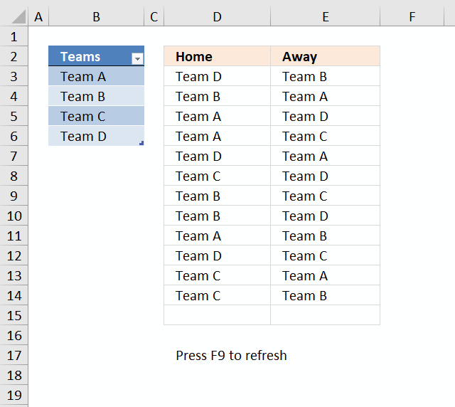
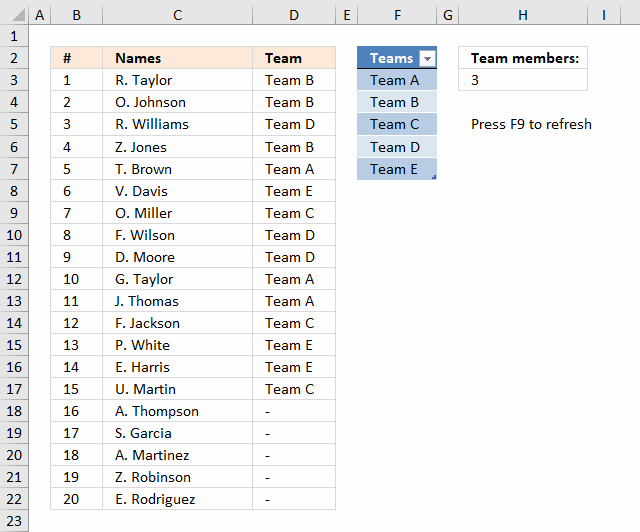
Create a random playlist
This article describes how to create a random playlist based on a given number of teams using an array formula. […]
![]()
Delete blanks and errors in a list
Table of Contents Delete blanks and errors in a list How to find errors in a worksheet 1. Delete blanks […]
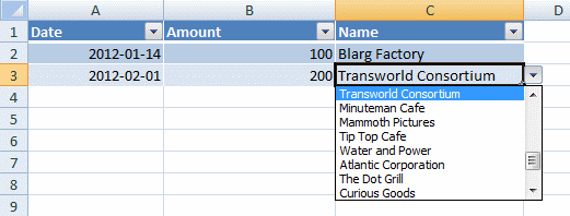
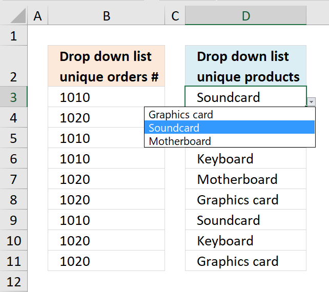
Dependent drop-down lists in multiple rows
This article demonstrates how to set up dependent drop-down lists in multiple cells. The drop-down lists are populated based on […]
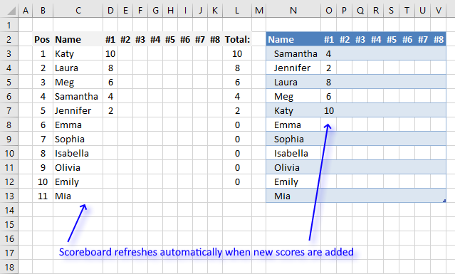
Dynamic scoreboard
This article demonstrates a scoreboard, displayed to the left, that sorts contestants based on total scores and refreshes instantly each […]
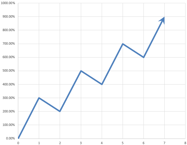
Dynamic stock chart
This stock chart built in Excel allows you to change the date range and the chart is instantly updated. What’s […]
Dynamic team generator
Mark G asks: 1 — I see you could change the formula to have the experssion COUNTIF($C$1:C1, $E$2:$E$5)<5 changed so […]
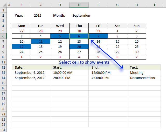
Excel calendar [VBA]
This workbook contains two worksheets, one worksheet shows a calendar and the other worksheet is used to store events. The […]
![]()

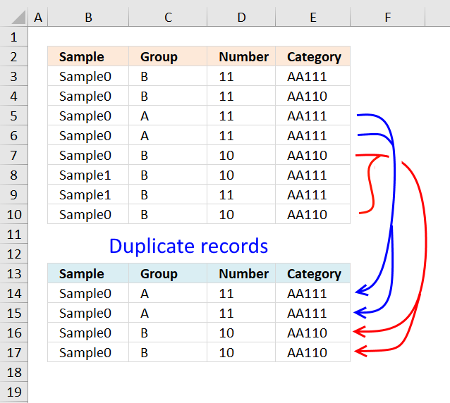
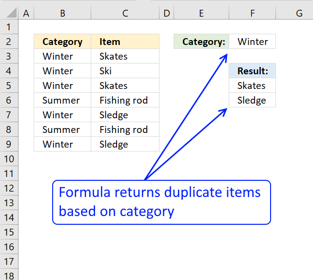
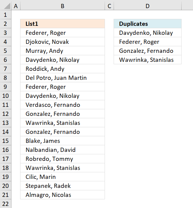
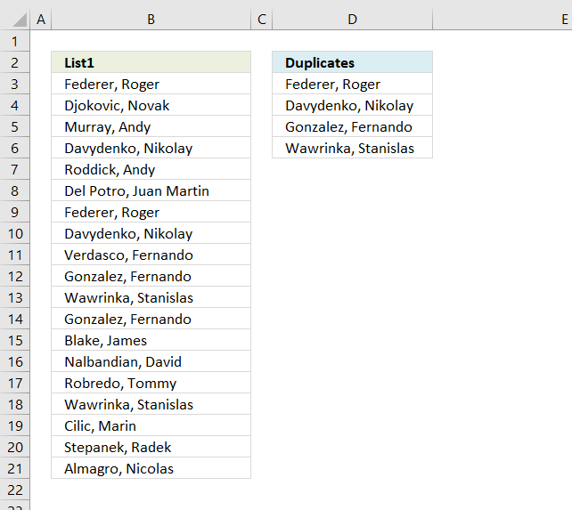
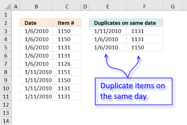
Extract duplicate records
This article describes how to filter duplicate rows with the use of a formula. It is, in fact, an array […]
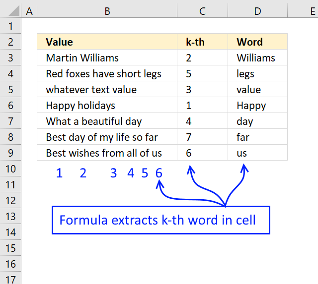
Extract n-th word in cell value
The formula displayed above in cell range D3:D9 extracts a word based on its position in a cell value. For […]
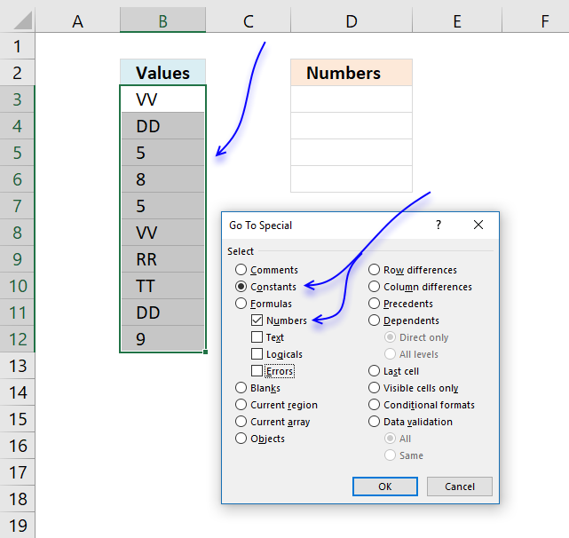
Extract numbers from a column
I this article I will show you how to get numerical values from a cell range manually and using an […]
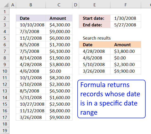
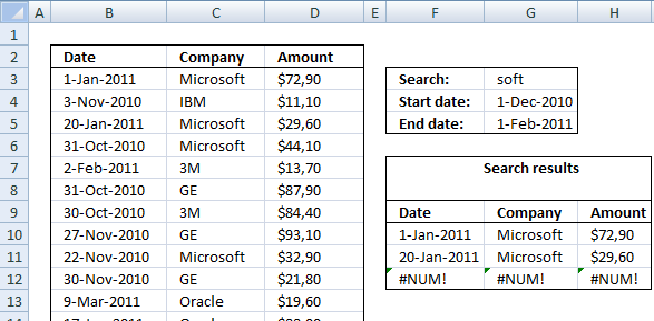
Extract records between two dates
This article presents methods for filtering rows in a dataset based on a start and end date. The image above […]
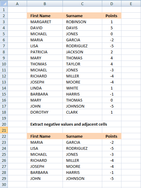
Extract records containing negative numbers
Table of Contents Extract negative values and adjacent cells (array formula) Extract negative values and adjacent cells (Excel Filter) Array […]
![]()
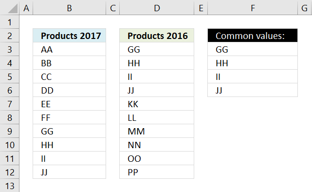
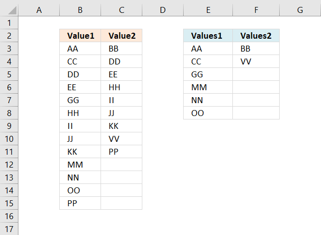
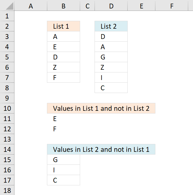
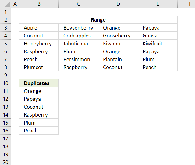
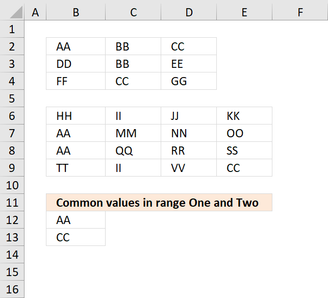
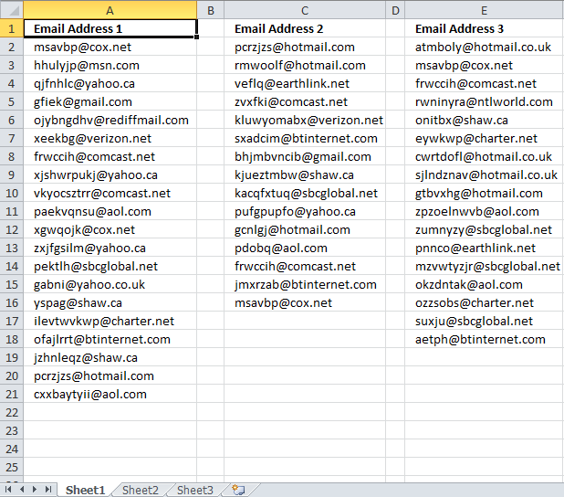
Extract shared values between two columns
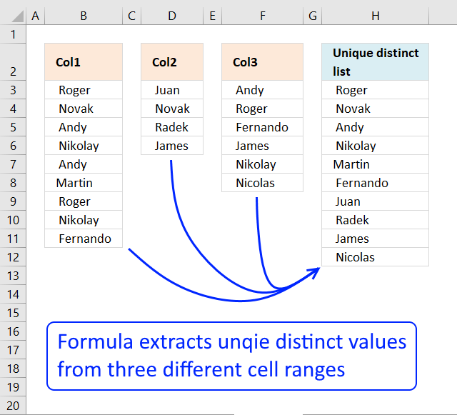
This article demonstrates ways to extract shared values in different cell ranges, two and three cell ranges. The Excel 365 […]
![]()
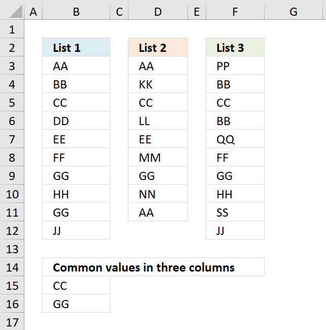
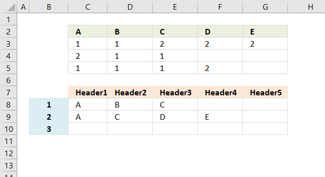
Filter common values from three separate columns
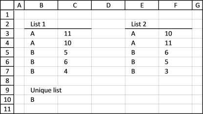
Array formula in B15: =INDEX($B$3:$B$12, MATCH(0, COUNTIF($B$14:B14, $B$3:$B$12)+IF(((COUNTIF($D$3:$D$11, $B$3:$B$12)>0)+(COUNTIF($F$3:$F$12, $B$3:$B$12)>0))=2, 0, 1), 0)) Copy cell B15 and paste it to […]
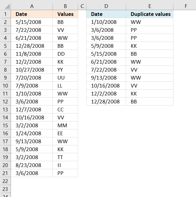
Filter duplicate values and sort by corresponding date
Array formula in D2: =INDEX($A$2:$A$21, MATCH(SMALL(IF(COUNTIF($B$2:$B$21, $B$2:$B$21)>1, COUNTIF($A$2:$A$21, «<«&$A$2:$A$21), «»),ROWS($A$1:A1)), COUNTIF($A$2:$A$21, «<«&$A$2:$A$21), 0)) Array formula in E2: =INDEX($B$2:$B$21, MATCH(SMALL(IF(COUNTIF($B$2:$B$21, $B$2:$B$21)>1, […]
Filter duplicate values based on criteria
This article demonstrates formulas and Excel tools that extract duplicates based on three conditions. The first and second condition is […]
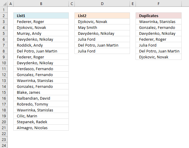
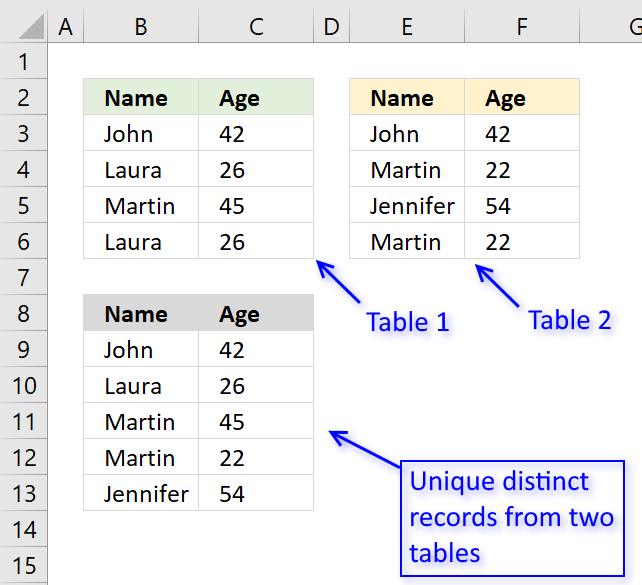
Filter shared records from two tables
I will in this blog post demonstrate a formula that extracts common records (shared records) from two data sets in […]
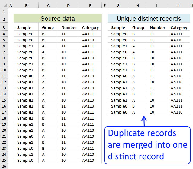
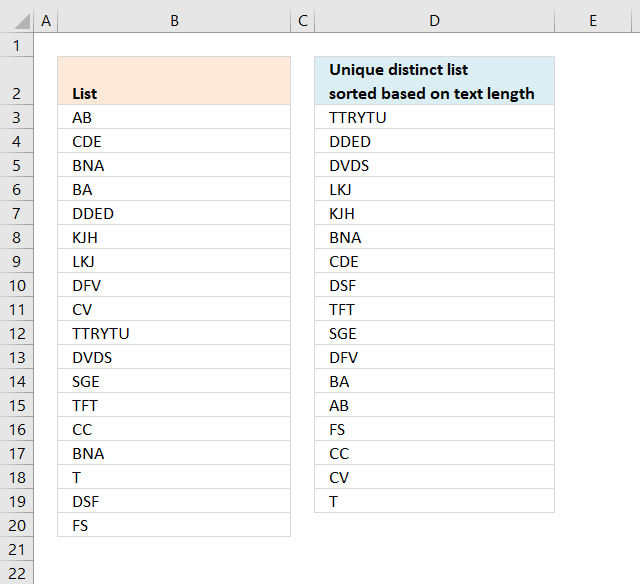
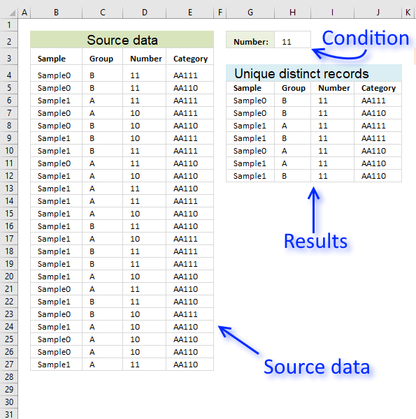
Filter unique distinct records
Table of contents Filter unique distinct row records Filter unique distinct row records but not blanks Filter unique distinct row […]
![]()
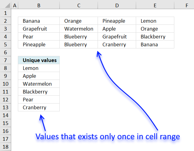
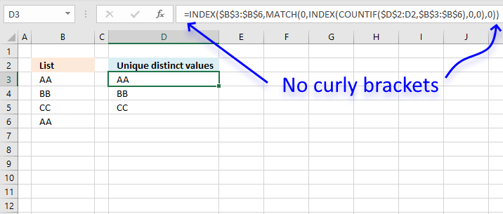
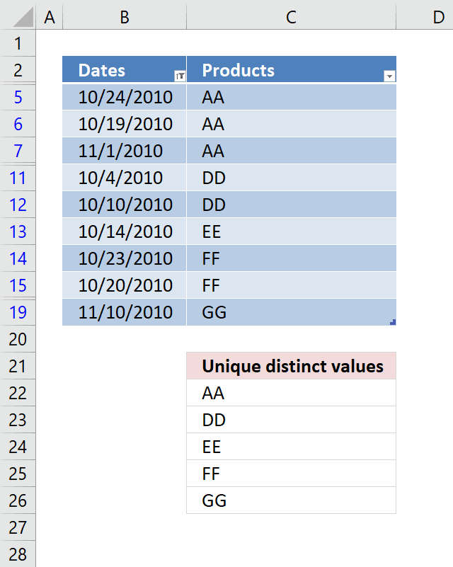
Filter unique values from a cell range
Unique values are values occurring only once in cell range. This is what I am going to demonstrate in this blog […]
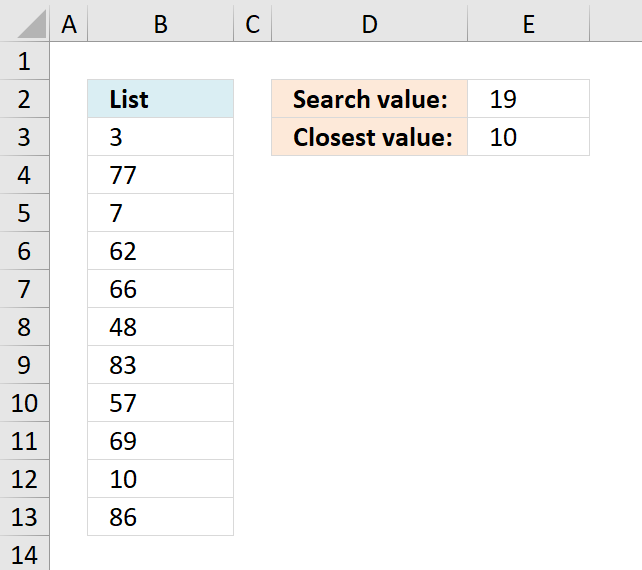
Find closest value
This article demonstrates formulas that extract the nearest number in a cell range to a condition. The image above shows […]
![]()
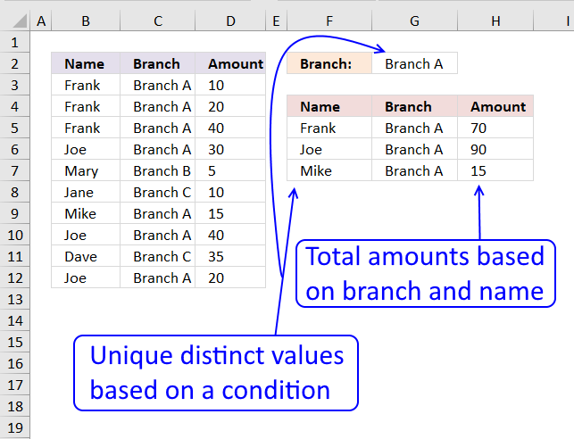
Find entry based on conditions
Bill Truax asks: Hello Oscar, I am building a spreadsheet for tracking calls for my local fire department. I have a […]
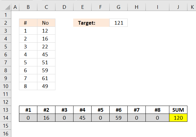
Find numbers closest to sum
Excelxor is such a great website for inspiration, I am really impressed by this post Which numbers add up to […]
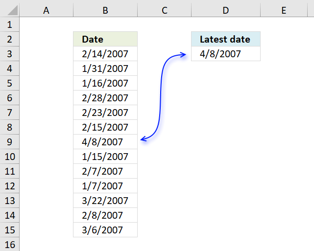
Find the most recent date in a list
The image above shows a formula in cell D3 that extracts the most recent date in cell range B3:B15. =MAX(B3:B15) […]
Free School Schedule Template
This template makes it easy for you to create a weekly school schedule, simply enter the time ranges and the […]
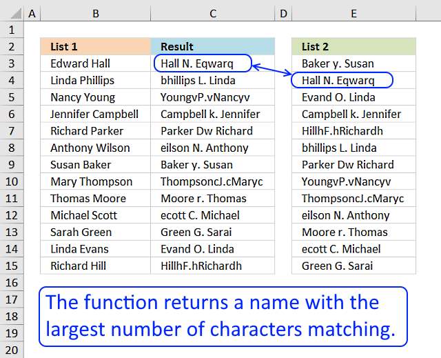
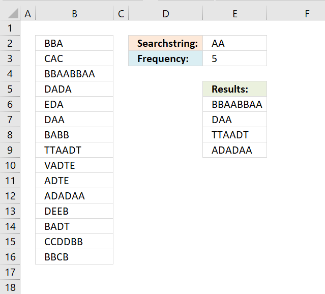
Fuzzy lookups
In this post I will describe a basic user defined function with better search functionality than the array formula in […]
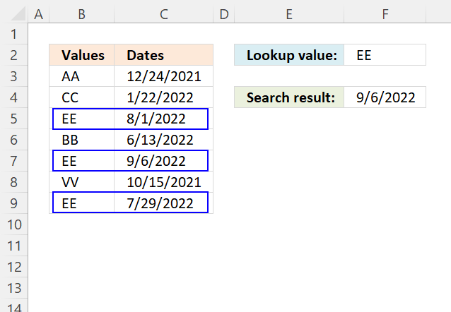
Fuzzy VLOOKUP
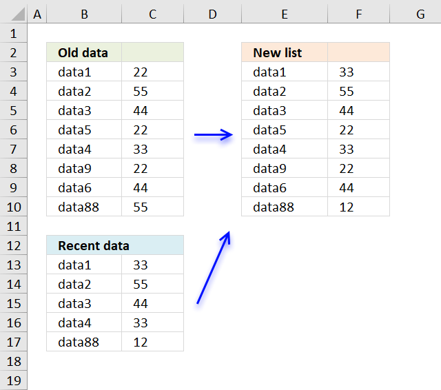
This formula returns multiple values even if they are arranged differently or have minor misspellings compared to the lookup value.
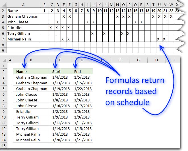
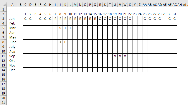
Get date ranges from a schedule
This article demonstrates ways to extract names and corresponding populated date ranges from a schedule using Excel 365 and earlier […]
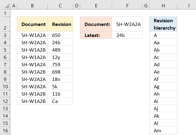
Get the latest revision
Column B contains document names, many of them are duplicates. The adjacent column C has the revision of the documents […]

Highlight lookups in relational tables
This article demonstrates a worksheet that highlights lookups across relational tables. I am using Excel defined Tables, if you add […]
How to animate an Excel chart
This article demonstrates how to create a chart that animates the columns when filtering chart data. The columns change incrementally […]
Functions in this article
Functions in ‘Lookup and reference’ category
The INDEX function function is one of many functions in the ‘Lookup and reference’ category.
Returns the address of a specific cell, you need to provide a row and column number.
Returns the number of cell ranges and single cells in a reference.
Gets a value based on a number.
Returns the column number of the top-left cell of a cell reference.
Calculates the number of columns in a cell range.
Extracts values/rows based on a condition or criteria.
Returns a formula as a text string.
Searches the top row in a data range for a value and return another value on the same column in a row you specify.
Builds a link in a cell.
Returns a value or reference from a cell range or array, you specify which value based on a row and column number.
Returns the cell reference based on a text string and shows the content of that cell reference.
Find a value in a cell range and return a corresponding value on the same row.
Returns the relative position of an item in an array that matches a specified value in a specific order.
Returns a reference to a range that is a given number of rows and columns from a given reference.
Calculates the row number of a cell reference.
Calculate the number of rows in a cell range.
Sorts values from a cell range or array
Sorts a cell range or array based on values in a corresponding range or array.
Downloads stock prices based on a stock quote
Converts a vertical range to a horizontal range, or vice versa.
Returns a unique or unique distinct list.
Lets you search the leftmost column for a value and return another value on the same row in a column you specify.
Search one column for a given value, and return a corresponding value in another column from the same row.
Searches for an item in an array or cell range and returns the relative position.
Excel function categories
Excel functions that let you resize, combine, and shape arrays.
Functions for backward compatibility with earlier Excel versions. Compatibility functions are replaced with newer functions with improved accuracy. Use the new functions if compatibility isn’t required.
Perform basic operations to a database-like structure.
Functions that let you perform calculations to Excel date and time values.
Let’s you manipulate binary numbers, convert values between different numeral systems, and calculate imaginary numbers.
Calculate present value, interest, accumulated interest, principal, accumulated principal, depreciation, payment, price, growth, yield for securities, and other financial calculations.
Functions that let you get information from a cell, formatting, formula, worksheet, workbook, filepath, and other entitites.
Functions that let you return and manipulate logical values, and also control formula calculations based on logical expressions.
These functions let you sort, lookup, get external data like stock quotes, filter values based a condition or criteria, and get the relative position of a given value in a specific cell range. They also let you calculate row, column, and other properties of cell references.
You will find functions in this category that calculates random values, round numerical values, create sequential numbers, trigonometry, and more.
Calculate distributions, binomial distributions, exponential distribution, probabilities, variance, covariance, confidence interval, frequency, geometric mean, standard deviation, average, median, and other statistical metrics.
Functions that let you manipulate text values, substitute strings, find string in value, extract a substring in a string, convert characters to ANSI code among other functions.
Get data from the internet, extract data from an XML string and more.
Excel categories
Latest updated articles.
More than 300 Excel functions with detailed information including syntax, arguments, return values, and examples for most of the functions used in Excel formulas.
More than 1300 formulas organized in subcategories.
Excel Tables simplifies your work with data, adding or removing data, filtering, totals, sorting, enhance readability using cell formatting, cell references, formulas, and more.
Allows you to filter data based on selected value , a given text, or other criteria. It also lets you filter existing data or move filtered values to a new location.
Lets you control what a user can type into a cell. It allows you to specifiy conditions and show a custom message if entered data is not valid.
Lets the user work more efficiently by showing a list that the user can select a value from. This lets you control what is shown in the list and is faster than typing into a cell.
Lets you name one or more cells, this makes it easier to find cells using the Name box, read and understand formulas containing names instead of cell references.
The Excel Solver is a free add-in that uses objective cells, constraints based on formulas on a worksheet to perform what-if analysis and other decision problems like permutations and combinations.
An Excel feature that lets you visualize data in a graph.
Format cells or cell values based a condition or criteria, there a multiple built-in Conditional Formatting tools you can use or use a custom-made conditional formatting formula.
Lets you quickly summarize vast amounts of data in a very user-friendly way. This powerful Excel feature lets you then analyze, organize and categorize important data efficiently.
VBA stands for Visual Basic for Applications and is a computer programming language developed by Microsoft, it allows you to automate time-consuming tasks and create custom functions.
A program or subroutine built in VBA that anyone can create. Use the macro-recorder to quickly create your own VBA macros.
UDF stands for User Defined Functions and is custom built functions anyone can create.
A list of all published articles.
So, there are times when you would like to know that a value is in a list or not. We have done this using VLOOKUP. But we can do the same thing using COUNTIF function too. So in this article, we will learn how to check if a values is in a list or not using various ways.
Check If Value In Range Using COUNTIF Function
So as we know, using COUNTIF function in excel we can know how many times a specific value occurs in a range. So if we count for a specific value in a range and its greater than zero, it would mean that it is in the range. Isn’t it?
Generic Formula
=COUNTIF(range,value)>0
Range: The range in which you want to check if the value exist in range or not.
Value: The value that you want to check in the range.
Let’s see an example:
Excel Find Value is in Range Example
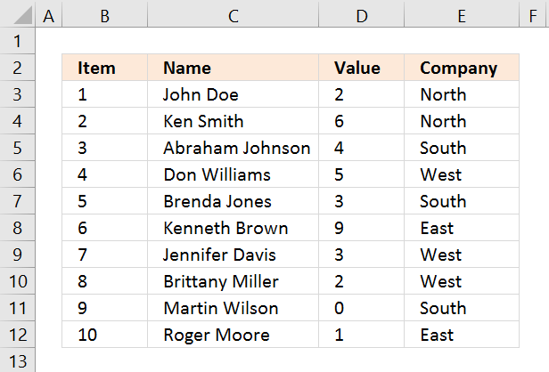
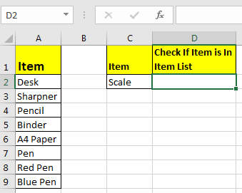
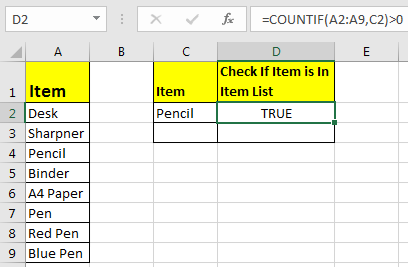
For this example, we have below sample data. We need a check-in the cell D2, if the given item in C2 exists in range A2:A9 or say item list. If it’s there then, print TRUE else FALSE.
Write this formula in cell D2:
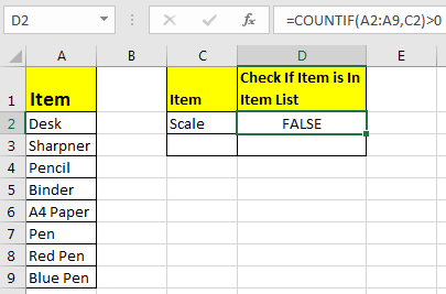
Since C2 contains “scale” and it’s not in the item list, it shows FALSE. Exactly as we wanted. Now if you replace “scale” with “Pencil” in the formula above, it’ll show TRUE.
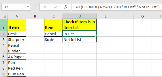
Now, this TRUE and FALSE looks very back and white. How about customizing the output. I mean, how about we show, “found” or “not found” when value is in list and when it is not respectively.
Since this test gives us TRUE and FALSE, we can use it with IF function of excel.
Write this formula:
=IF(COUNTIF(A2:A9,C2)>0,»in List»,»Not in List»)
You will have this as your output.
What If you remove “>0” from this if formula?
=IF(COUNTIF(A2:A9,C2),»in List»,»Not in List»)
It will work fine. You will have same result as above. Why? Because IF function in excel treats any value greater than 0 as TRUE.
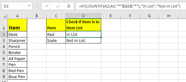
How to check if a value is in Range with Wild Card Operators
Sometimes you would want to know if there is any match of your item in the list or not. I mean when you don’t want an exact match but any match.
For example, if in the above-given list, you want to check if there is anything with “red”. To do so, write this formula.
=IF(COUNTIF(A2:A9,»*red*»),»in List»,»Not in List»)
This will return a TRUE since we have “red pen” in our list. If you replace red with pink it will return FALSE. Try it.
Now here I have hardcoded the value in list but if your value is in a cell, say in our favourite cell B2 then write this formula.
IF(COUNTIF(A2:A9,»*»&B2&»*»),»in List»,»Not in List»)
There’s one more way to do the same. We can use the MATCH function in excel to check if the column contains a value. Let’s see how.
Find if a Value is in a List Using MATCH Function
So as we all know that MATCH function in excel returns the index of a value if found, else returns #N/A error. So we can use the ISNUMBER to check if the function returns a number.
If it returns a number ISNUMBER will show TRUE, which means it’s found else FALSE, and you know what that means.
Write this formula in cell C2:
=ISNUMBER(MATCH(C2,A2:A9,0))
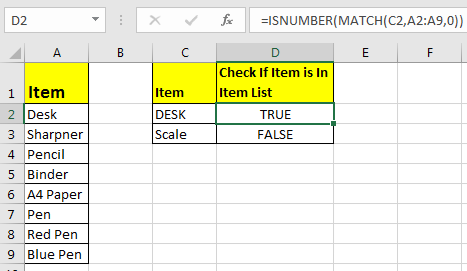
The MATCH function looks for an exact match of value in cell C2 in range A2:A9. Since DESK is on the list, it shows a TRUE value and FALSE for SCALE.
So yeah, these are the ways, using which you can find if a value is in the list or not and then take action on them as you like using IF function. I explained how to find value in a range in the best way possible. Let me know if you have any thoughts. The comments section is all yours.
Related Articles:
How to Check If Cell Contains Specific Text in Excel
How to Check A list of Texts In String in Excel
How to take the Average Difference between lists in Excel
How to Get Every Nth Value From A list in Excel
Popular Articles:
50 Excel Shortcuts to Increase Your Productivity
How to use the VLOOKUP Function in Excel
How to use the COUNTIF function in Excel
How to use the SUMIF Function in Excel
Excel has a lot of functions – about 450+ of them.
And many of these are simply awesome. The amount of work you can get done with a few formulas still surprises me (even after having used Excel for 10+ years).
And among all these amazing functions, the INDEX MATCH functions combo stands out.
I am a huge fan of INDEX MATCH combo and I have made it pretty clear many times.
I even wrote an article about Index Match Vs VLOOKUP which sparked a little bit of debate (you can check the comments section for some firework).
And today, I am writing this article solely focussed on Index Match to show you some simple and advanced scenarios where you can use this powerful formula combo and get the work done.
Note: There are other lookup formulas in Excel – such as VLOOKUP and HLOOKUP and these are great. Many people find VLOOKUP to be easier to use (and that’s true as well). I believe INDEX MATCH is a better option in many cases. But since people find it difficult, it gets used less. So I am trying to simplify it using this tutorial.
Now before I show you how the combination of INDEX MATCH is changing the world of analysts and data scientists, let me first introduce you to the individual parts – INDEX and MATCH functions.
INDEX Function: Finds the Value-Based on Coordinates
The easiest way to understand how Index function works is by thinking of it as a GPS satellite.
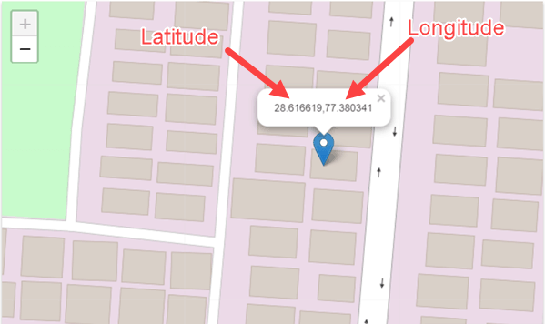
As soon as you tell the satellite the latitude and longitude coordinates, it will know exactly where to go and find that location.
So despite having a mind-boggling number of lat-long combinations, the satellite would know exactly where to look.
I quickly did a search for my work location and this is what I got.
Anyway, enough of geography.
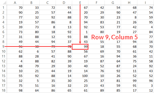
Just like a satellite needs latitude and longitude coordinates, the INDEX function in Excel would need the row and column number to know what cell you’re referring to.
And that’s Excel INDEX function in a nut-shell.
So let me define it in simple words for you.
The INDEX function will use the row number and column number to find a cell in the given range and return the value in it.
All by itself, INDEX is a very simple function, with no utility. After all, in most cases, you are not likely to know the row and column numbers.
But…
The fact that you can use it with other functions (hint: MATCH) that can find the row number and the column number makes INDEX an extremely powerful Excel function.
Below is the syntax of the INDEX function:
=INDEX (array, row_num, [col_num])
=INDEX (array, row_num, [col_num], [area_num])
- array – a range of cells or an array constant.
- row_num – the row number from which the value is to be fetched.
- [col_num] – the column number from which the value is to be fetched. Although this is an optional argument, but if row_num is not provided, it needs to be given.
- [area_num] – (Optional) If array argument is made up of multiple ranges, this number would be used to select the reference from all the ranges.
INDEX function has 2 syntaxes (just FYI).
The first one is used in most cases. The second one is used in advanced cases only (such as doing a three-way lookup) which we will cover in one of the examples later in this tutorial.
But if you’re new to this function, just remember the first syntax.
Below is a video that explains how to use the INDEX function
MATCH Function: Finds the Position baed on a Lookup Value
Going back to my previous example of longitude and latitude, MATCH is the function that can find these positions (in the Excel spreadsheet world).
In simple language, the Excel MATCH function can find the position of a cell in a range.
And on what basis would it find a cell’s position?
Based on the lookup value.
For example, if you have a list as shown below and you want to find the position of the name ‘Mark’ in it, then you can use the MATCH function.
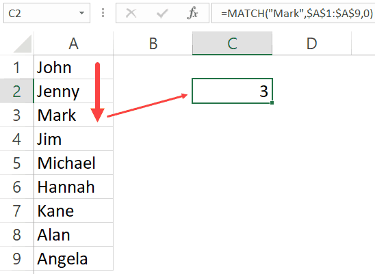
The function returns 3, as that’s the position of the cell with the name Mark in it.
MATCH function starts looking from top to bottom for the lookup value (which is ‘Mark’) in the specified range (which is A1:A9 in this example). As soon as it finds the name, it returns the position in that specific range.
Below is the syntax of the MATCH function in Excel.
=MATCH(lookup_value, lookup_array, [match_type])
- lookup_value – The value for which you are looking for a match in the lookup_array.
- lookup_array – The range of cells in which you are searching for the lookup_value.
- [match_type] – (Optional) This specifies how excel should look for a matching value. It can take three values -1, 0 , or 1.
Understanding Match Type Argument in MATCH Function
There is one additional thing you need to know about the MATCH function, and it’s about how it goes through the data and finds the cell position.
The third argument of the MATCH function can be 0, 1 or -1.
Below is an explanation of how these arguments work:
- 0 – this will look for an exact match of the value. If an exact match is found, the MATCH function will return the cell position. Else, it will return an error.
- 1 – this finds the largest value that is less than or equal to the lookup value. For this to work, your data range needs to be sorted in ascending order.
- -1 – this finds the smallest value that is greater than or equal to the lookup value. For this to work, your data range needs to be sorted in descending order.
Below is a video that explains how to use the MATCH function (along with the match type argument)
To summarize and put it in simple words:
- INDEX needs the cell position (row and column number) and gives the cell value.
- MATCH finds the position by using a lookup value.
Let’s Combine Them to Create a Powerhouse (INDEX + MATCH)
Now that you have a basic understanding of how INDEX and MATCH functions work individually, let’s combine these two and learn about all the wonderful things it can do.
To understand this better, I have a few examples that use the INDEX MATCH combination.
I will start with a simple example and then show you some advanced use cases as well.
Click here to download the example file
Example 1: A simple Lookup Using INDEX MATCH Combo
Let’s do a simple lookup with INDEX/MATCH.
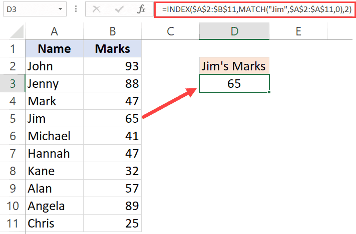
Below is a table where I have the marks for ten students.
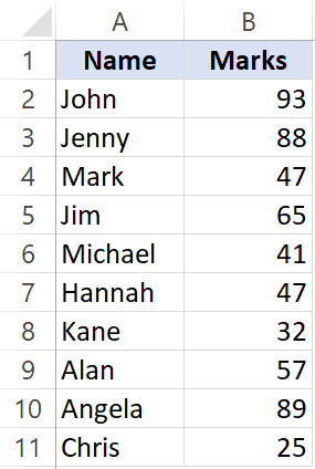
From this table, I want to find the marks for Jim.
Below is the formula that can easily do this:
=INDEX($A$2:$B$11,MATCH("Jim",$A$2:$A$11,0),2)
Now, if you’re thinking this can easily be done using a VLOOKUP function, you’re right! This is not the best use of INDEX MATCH awesomeness. Despite the fact that I am a fan of INDEX MATCH, it is a little more difficult than VLOOKUP. If fetching data from a column on the right is all you want to do, I recommend you use VLOOKUP.
The reason I have shown this example, which can also easily be done with VLOOKUP is to show you how INDEX MATCH works in a simple setting.
Now let me show a benefit of INDEX MATCH.
Suppose you have the same data, but instead of having it in columns, you have it in rows (as shown below).

You know what, you can still use INDEX MATCH combo to get Jim’s marks.
Below is the formula that will give you the result:
=INDEX($B$1:$K$2,2,MATCH(“Jim”,$B$1:$K$1,0))
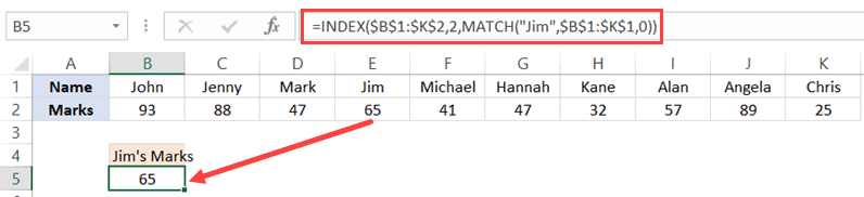
Note that you need to change the range and switch the row/column parts to make this formula work for horizontal data as well.
This can’t be done with VLOOKUP, but you can still do this easily with HLOOKUP.
INDEX MATCH combination can easily handle horizontal as well as vertical data.
Click here to download the example file
Example 2: Lookup to the Left
It’s more common than you think.
A lot of times, you may be required to fetch the data from a column which is to the left of the column that has the lookup value.
Something as shown below:
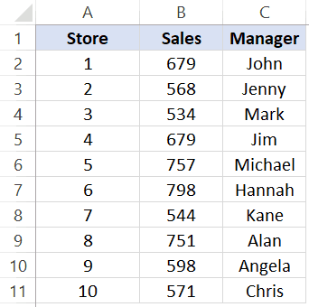
To find out Michael’s sales, you will have to do a lookup on the left.
If you’re thinking VLOOKUP, let me stop your right there.
VLOOKUP is not made to look for and fetch the values on the left.
Can you still do it using VLOOKUP?
Yes, you can!
But that can turn into a long and ugly formula.
So if you want to do a lookup and fetch data from the columns on the left, you are better off using INDEX MATCH combo.
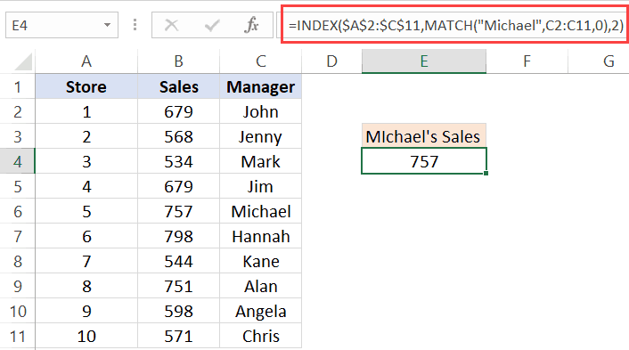
Below is the formula that will get Michael’s sales number:
=INDEX($A$2:$C$11,MATCH("Michael",C2:C11,0),2)
Another point here for INDEX MATCH. VLOOKUP can fetch the data only from the columns that are to the right of the column that has the lookup value.
Example 3: Two Way Lookup
So far, we have seen the examples where we wanted to fetch the data from the column adjacent to the column that has the lookup value.
But in real life, the data often spans through multiple columns.
INDEX MATCH can easily handle a two-way lookup.
Below is a dataset of the student’s marks in three different subjects.
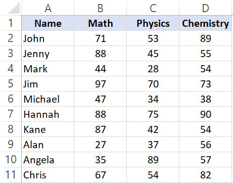
If you want to quickly fetch the marks of a student in all three subjects, you can do that with INDEX MATCH.
The below formula will give you the marks for Jim for all the three subjects (copy and paste in one cell and drag to fill other cells or copy and paste on other cells).
=INDEX($B$2:$D$11,MATCH($F$3,$A$2:$A$11,0),MATCH(G$2,$B$1:$D$1,0))

Let me quickly also explain this formula.
INDEX formula uses B2:D11 as the range.
The first MATCH uses the name (Jim in cell F3) and fetches the position of it in the names column (A2:A11). This becomes the row number from which the data needs to be fetched.
The second MATCH formula uses the subject name (in cell G2) to get the position of that specific subject name in B1:D1. For example, Math is 1, Physics is 2 and Chemistry is 3.
Since these MATCH positions are fed into the INDEX function, it returns the score based on the student name and subject name.
This formula is dynamic, which means that if you change the student name or the subject names, it would still work and fetch the correct data.
One great thing about using INDEX/MATCH is that even if you interchange the names of the subjects, it will continue to give you the correct result.
Example 4: Lookup Value From Multiple Column/Criteria
Suppose you have a dataset as shown below and you want to fetch the marks for ‘Mark Long’.

Since the data is in two columns, I can’t a lookup for Mark and get the data.
If I do it that way, I am going to get the marks data for Mark Frost and not Mark Long (because the MATCH function will give me the result for the MARK it meets).
One way of doing this is to create a helper column and combine the names. Once you have the helper column, you can use VLOOKUP and get the marks data.
If you’re interested in learning how to do this, read this tutorial on using VLOOKUP with multiple criteria.
But with INDEX/MATCH combo, you don’t need a helper column. You can create a formula that handles multiple criteria in the formula itself.
The below formula will give the result.
=INDEX($C$2:$C$11,MATCH($E$3&"|"&$F$3,$A$2:A11&"|"&$B$2:$B$11,0))

Let me quickly explain what this formula does.
The MATCH part of the formula combines the lookup value (Mark and Long) as well as the entire lookup array. When $A$2:A11&”|”&$B$2:$B$11 is used as the lookup array, it actually checks the lookup value against the combined string of first and last name (separated by the pipe symbol).
This ensures that you get the right result without using any helper columns.
You can do this kind of lookup (where there are multiple columns/criteria) with VLOOKUP as well, but you need to use a helper column. INDEX MATCH combo makes it slightly easy to do this without any helper columns.
Example 5: Get Values from Entire Row/Column
In the examples above, we have used the INDEX function to get value from a specific cell. You provide the row and column number, and it returns the value in that specific cell.
But you can do more.
You can also use the INDEX function to get the values from an entire row or column.
And how can this be useful you ask!
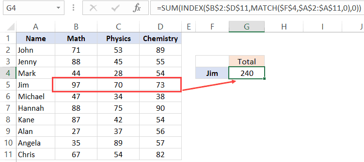
Suppose you want to know the total score of Jim in all the three subjects.
You can use the INDEX function to first get all the marks of Jim and then use the SUM function to get a total.
Let’s see how to do this.
Below I have the scores of all the students in three subjects.
The below formula will give me the total score of Jim in all the three subjects.
=SUM(INDEX($B$2:$D$11,MATCH($F$4,$A$2:$A$11,0),0))
Let me explain how this formula works.
The trick here is to use 0 as the column number.
When you use 0 as the column number in the INDEX function, it will return all the row values. Similarly, if you use 0 as the row number, it will return all the values in the column.
So the below part of the formula returns an array of values – {97, 70, 73}
INDEX($B$2:$D$11,MATCH($F$4,$A$2:$A$11,0),0)
If you just enter this above formula in a cell in Excel and hit enter, you will see a #VALUE! error. This is because it’s not returning a single value, but an array of value.
But don’t worry, the array of values are still there. You can check this by selecting the formula and press the F9 key. It will show you the result of the formula which in this case is an array of three value – {97, 70, 73}
Now, if you wrap this INDEX formula in the SUM function, it will give you the sum of all the marks scored by Jim.
You can also use the same to get the highest, lowest and average marks of Jim.
Just like we have done this for a student, you can also do this for a subject. For example, if you want the average score in a subject, you can keep the row number as 0 in the INDEX formula and it will give you all the column values of that subject.
Click here to download the example file
Example 6: Find the Student’s Grade (Approximate Match Technique)
So far, we have used the MATCH formula to get the exact match of the lookup value.
But you can also use it to do an approximate match.
Now, what the hell is Approximate Match?
Let me explain.
When you’re looking for stuff such as names or ids, you’re looking for an exact match. But sometimes, you need to know the range in which your lookup values lie. This is usually the case with numbers.
For example, as a class teacher, you may want to know what’s the grade of each student in a subject, and the grade is decided based on the score.
Below is an example, where I want the grade for all the students and the grading is decided based on the table on the right.
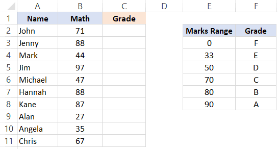
So if a student gets less than 33, the grade is F and if he/she gets less than 50 but more than 33, it’s E, and so on.
Below is the formula that will do this.
=INDEX($F$3:$F$8,MATCH(B2,$E$3:$E$8,1),1)
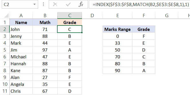
Let me explain how this formula works.
In the MATCH function, we have used 1 as the [match_type] argument. This argument will return the largest value that is less than or equal to the lookup value.
This means that the MATCH formula goes through the marks range, and as soon as it finds a marks range that is equal to or less than the lookup marks value, it will stop there and return its position.
So if the lookup mark value is 20, the MATCH function would return 1 and if it’s 85, it would return 5.
And the INDEX function uses this position value to get the grade.
IMPORTANT: For this to work, your data needs to be sorted in ascending order. If it’s not, you can get wrong results.
Note that the above can also be done using below VLOOKUP formula:
=VLOOKUP(B2,$E$3:$F$8,2,TRUE)
But MATCH function can go a step further when it comes to approximate match.
You can also have a descending data and can use INDEX MATCH combo to find the result. For example, if I change the order of the grade table (as shown below), I can still find the grades of the students.
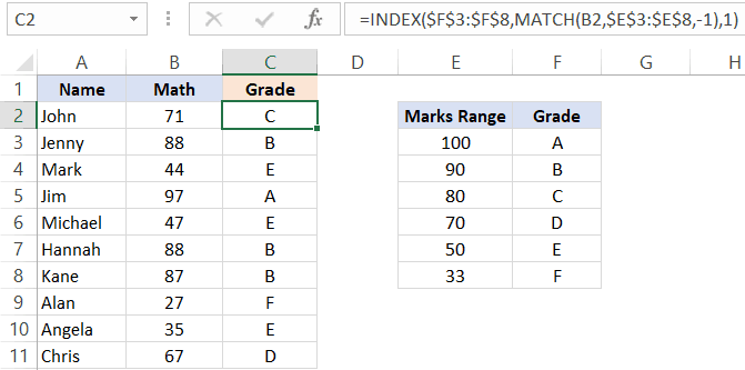
To do this, all I have to do is change the [match_type] argument to -1.
Below is the formula that I have used:
=INDEX($F$3:$F$8,MATCH(B2,$E$3:$E$8,-1),1)
VLOOKUP can also do an approximate match but only when data is sorted in ascending order(but it doesn’t work if the data is sorted in descending order).
Example 7: Case Sensitive Lookups
So far all the lookups we have done have been case insensitive.
This means that whether the lookup value was Jim or JIM or jim, it didn’t matter. You’ll get the same result.
But what if you want the lookup to be case sensitive.
This is usually the case when you have large data sets and a possibility of repetition or distinct names/ids (with the only difference being the case)
For example, suppose I have the following data set of students where there are two students with the name Jim (the only difference being that one is entered as Jim and another one as jim).

Note that there are two students with the same name – Jim (cell A2 and A5).
Since a normal lookup wouldn’t work, you need to do a case sensitive lookup.
Below is the formula that will give you the right result. Since this is an array formula, you need to use Control + Shift + Enter.
=INDEX($B$2:$B$11,MATCH(TRUE,EXACT(D3,A2:A11),0),1)

Let me explain how this formula works.
The EXACT function checks for an exact match of the lookup value (which is ‘jim’ in this case). It goes through all the names and returns FALSE if it isn’t a match and TRUE if it’s a match.
So the output of the EXACT function in this example is – {FALSE;FALSE;FALSE;TRUE;FALSE;FALSE;FALSE;FALSE;FALSE;FALSE}
Note that there is only one TRUE, which is when the EXACT function found a perfect match.
The MATCH function then finds the position of TRUE in the array returned by the EXACT function, which is 4 in this example.
Once we have the position, the INDEX function uses it to find the marks.
Example 8: Find the Closest Match
Let’s get a little advanced now.
Suppose you have a dataset where you want to find the person who has the work experience closest to the required experience (mentioned in cell D2).
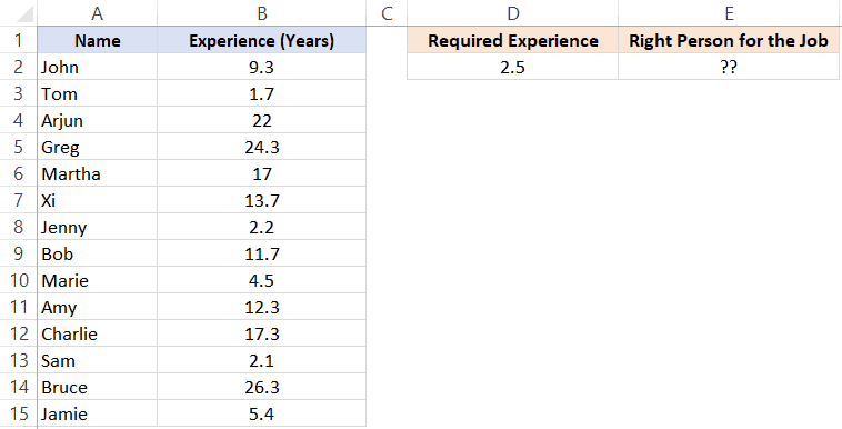
While lookup formulas are not made to do this, you can combine it with other functions (such as MIN and ABS) to get this done.
Below is the formula that will find the person with the experience closest to the required one and return the name of the person. Note that the experience needs to be closest (which can be either less or more).
=INDEX($A$2:$A$15,MATCH(MIN(ABS(D2-B2:B15)),ABS(D2-$B$2:$B$15),0))
Since this is an array formula, you need to use Control + Shift + Enter.
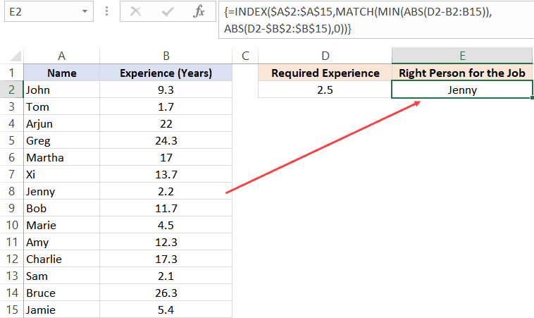
The trick in this formula is to change the lookup value and lookup array to find the minimum experience difference in required and actual values.
Before I explain the formula, let’s understand how you would do it manually.
You will go through each cell in column B and find the difference in the experience between what is required and the one that a person has. Once you have all the differences, you will find the one which is minimum and fetch the name of that person.
This is exactly what we are doing with this formula.
Let me explain.
The lookup value in the MATCH formula is MIN(ABS(D2-B2:B15)).
This part gives you the minimum difference between the given experience (which is 2.5 years) and all the other experiences. In this example, it returns 0.3
Note that I have used ABS to make sure I am looking for the closest (which can be more or less than the given experience).
Now, this minimum value becomes our lookup value.
The lookup array in the MATCH function is ABS(D2-$B$2:$B$15).
This gives us an array of numbers from which 2.5 (the required experience) has been subtracted.
So now we have a lookup value (0.3) and a lookup array ({6.8;0.8;19.5;21.8;14.5;11.2;0.3;9.2;2;9.8;14.8;0.4;23.8;2.9})
MATCH function finds the position of 0.3 in this array, which is also the position of the person’s name who has the closest experience.
This position number is then used by the INDEX function to return the name of the person.
Related Read: Find the Closest Match in Excel (examples using lookup formulas)
Click here to download the example file
Example 9: Use INDEX MATCH with Wildcard Characters
If you want to look up a value when there is a partial match, then you need to use wildcard characters.
For example, below is a dataset of company name and their market capitalizations and you want to want to get the market cap. data for the three companies on the right.
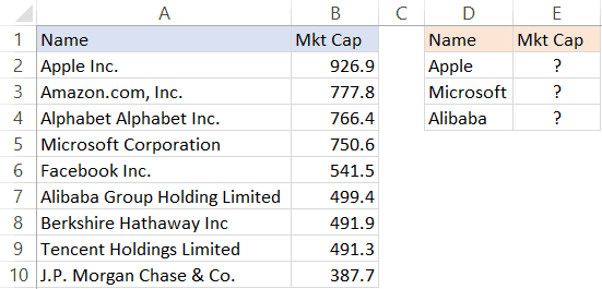
Since these are not exact matches, you can’t do a regular lookup in this case.
But you can still get the right data by using an asterisk (*), which is a wildcard character.
Below is the formula that will give you the data by matching the company names from the main column and fetching the market cap figure for it.
=INDEX($B$2:$B$10,MATCH(D2&”*”,$A$2:$A$10,0),1)
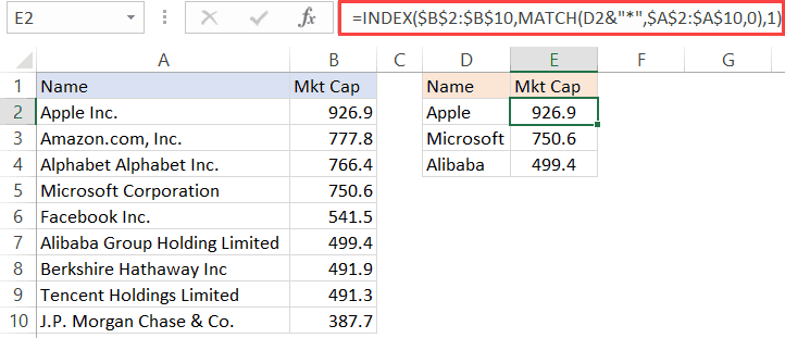
Let me explain how this formula works.
Since there is no exact match of lookup values, I have used D2&”*” as the lookup value in the MATCH function.
An asterisk is a wildcard character that represents any number of characters. This means that Apple* in the formula would mean any text string that starts with the word Apple and can have any number of characters after it.
So when Apple* is used as the lookup value and the MATCH formula looks for it in column A, it returns the position of ‘Apple Inc.’, as it starts with the word Apple.
You can also use wildcard characters to find text strings where the lookup value is in between. For example, if you use *Apple* as the lookup value, it will find any string that has the word apple anywhere in it.
Note: This technique works well when you only have one instance of matching. But if you have multiple instances of matching (for example Apple Inc and Apple Corporation, then the MATCH function would return the position of the first matching instance only.
Example 10: Three Way Lookup
This is an advanced use of INDEX MATCH, but I will still cover it to show you the power of this combination.
Remember I said that INDEX function has two syntaxes:
=INDEX (array, row_num, [col_num])
=INDEX (array, row_num, [col_num], [area_num])
So far in all our examples, we have only used the first one.
But for a three-way lookup, you need to use the second syntax.
Let me first explain what a three-way look means.
In a two-way lookup, we use the INDEX MATCH formula to get the marks when we have the student’s name and the subject name. For example, fetching the marks of Jim in Math is a two-way lookup.
A three-way look would add another dimension to it. For example, suppose you have a dataset as shown below and you want to know the score of Jim in Math in Mid-term exam, then this would be three-way lookup.
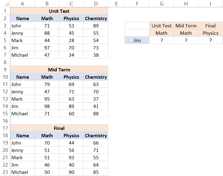
Below is the formula that will give the result.
=INDEX(($B$3:$D$7,$B$11:$D$15,$B$19:$D$23),MATCH($F$5,$A$3:$A$7,0),MATCH(G$4,$B$2:$D$2,0),(IF(G$3="Unit Test",1,IF(G$3="Mid Term",2,3))))
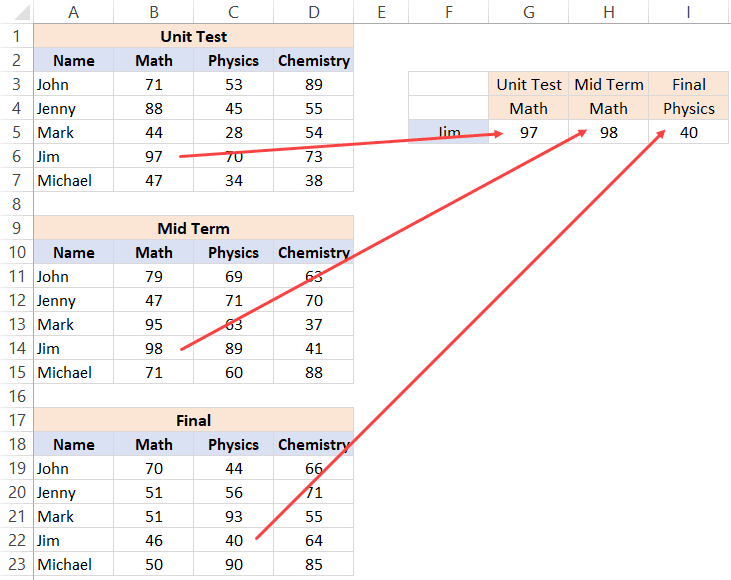
The above formula checked for three things – the name of the student, the subject, and the exam. After it finds the right value, it returns it in the cell.
Let me explain how this formula works by breaking down the formula into parts.
- array – ($B$3:$D$7,$B$11:$D$15,$B$19:$D$23): Instead of using a single array, in this case, I have used three arrays within parenthesis.
- row_num – MATCH($F$5,$A$3:$A$7,0): MATCH function is used to find the position of the student’s name in cell $F$5 in the list of student’s name.
- col_num – MATCH(G$4,$B$2:$D$2,0): MATCH function is used to find the position of the subject name in cell $B$2 in the list of subject’s name.
- [area_num] – IF(G$3=”Unit Test”,1,IF(G$3=”Mid Term”,2,3)): The area number value tells the INDEX function which of the three arrays to use to fetch the value. If the exam is Unit Term, the IF function would return 1 and the INDEX function would use the first array to fetch the value. If the exam is Mid-term, the IF formula would return 2, else it will return 3.
This is an advanced example of using INDEX MATCH, and you’re unlikely to find a situation when you have to use this. But it’s still good to know what Excel formulas can do.
Click here to download the example file
Why is INDEX/MATCH Better than VLOOKUP?
OR Is it?
Yes, it is – in most cases.
I will present my case in a while.
But before I do that, let me say this – VLOOKUP is an extremely useful function and I love it. It can do a lot of things in Excel and I use it every now and then myself. Having said that, it doesn’t mean that there can’t be anything better, and INDEX/MATCH (with more flexibility and functionalities) is better.
So if you want to do some basic lookup, you’re better off using VLOOKUP.
INDEX/MATCH is VLOOKUP on steroids. And once you learn INDEX/MATCH, you might always prefer using it (especially because of the flexibility it has).
Without stretching it too far, let me quickly give you the reasons why INDEX/MATCH is better than VLOOKUP.
INDEX/MATCH can look to the Left (as well as to the right) of the lookup value
I covered it in one of the example above.
If you have a value which is on the left of the lookup value, you can’t do that with VLOOKUP
At least not with just VLOOKUP.
Yes, you can combine VLOOKUP with other formulas and get it done, but it gets complicated and messy.
INDEX/MATCH, on the other hand, is made to lookup everywhere (be it left, right, up, or down)
INDEX/MATCH can work with vertical and horizontal ranges
Again, with full respect to VLOOKUP, it’s not made to do this.
After all, the V in VLOOKUP stands for vertical.
VLOOKUP can only go through data that is vertical, while INDEX/MATCH can go through data vertically as well horizontally.
Of course, there is the HLOOKUP function to take care of horizontal lookup, but it isn’t VLOOKUP then.. right?
I like the fact that INDEX MATCH combo is flexible enough to work with both vertical and horizontal data.
VLOOKUP cannot work with descending data
When it comes to the approximate match, VLOOKUP and INDEX/MATCH are at the same level.
But INDEX MATCH takes the point as it can also handle data that is in descending order.
I show this in one of the examples in this tutorial where we have to find the grade of students based on the grading table. If the table is sorted in descending order, VLOOKUP would not work (but INDEX MATCH would).
INDEX/MATCH can be slightly faster
I will be truthful. I didn’t run this test myself.
I am relying on the wisdom an Excel master – Charley Kyd.
The difference in speed in VLOOKUP and INDEX/MATCH is hardly noticeable when you have small data sets. But if you have thousands of rows and many columns, this can be a deciding factor.
In his article, Charley Kyd states:
“At its worst, the INDEX-MATCH method is about as fast as VLOOKUP; at its best, it’s much faster.”
INDEX/MATCH is Independent of the Actual Column Position
If you have a dataset as shown below as you’re fetching the score of Jim in Physics, you can do that using VLOOKUP.
And to do that, you can specify the column number as 3 in VLOOKUP.
All is fine.
But what if I delete the Math column.
In that case, the VLOOKUP formula will break.
Why? – Because it was hardcoded to use the third column, and when I delete a column in between, the third column becomes the second column.
Using INDEX/MATCH, in this case, is better as you can make the column number dynamic by using MATCH. So instead of a column number, it checks for the subject name and uses that to return the column number.
Surely you can do that by combining VLOOKUP with MATCH, but if you combining anyway, why not do it with INDEX which is a lot more flexible.
When using INDEX/MATCH, you can safely insert/delete columns in your dataset.
Despite all these factors, there is a reason VLOOKUP is so popular.
And it’s a big reason.
VLOOKUP is easier to use
VLOOKUP only takes a maximum of four arguments. If you can wrap your head around these four, you’re good to go.
And since most of the basic lookup cases are handled by VLOOKUP as well, it has quickly become the most popular Excel function.
I call it the King of Excel functions.
INDEX/MATCH, on the other hand, is a little more difficult to use. You may get a hang if it when you start using it, but for a beginner, VLOOKUP is far more easy to explain and learn.
And this is not a zero-sum game.
So, if you’re new to the lookup world and don’t know how to use VLOOKUP, better learn that.
I have a detailed guide on using VLOOKUP in Excel (with lots of examples)
My intent in this article is not to pitch two awesome functions against each other. I wanted to show you the power of INDEX MATCH combo and all the great things it can do.
Hope you found this article useful.
Let me know your thoughts in the comments section, and in case you find any mistake in this tutorial, please let me know.
You May Also Like the Following Excel Tutorials:
- Excel Functions
- 100+ Excel Interview Questions
- Find the Last Occurrnece of a Lookup Value in a List
- Lookup the Second, the Third, or the Nth Value in Excel
- Use IFERROR with VLOOKUP to Get Rid of #N/A Errors