
The INDEX function returns a value or the reference to a value from within a table or range.

There are two ways to use the INDEX function:
-
If you want to return the value of a specified cell or array of cells, see Array form.
-
If you want to return a reference to specified cells, see Reference form.
Array form
Description
Returns the value of an element in a table or an array, selected by the row and column number indexes.
Use the array form if the first argument to INDEX is an array constant.
Syntax
INDEX(array, row_num, [column_num])
The array form of the INDEX function has the following arguments:
-
array Required. A range of cells or an array constant.
-
If array contains only one row or column, the corresponding row_num or column_num argument is optional.
-
If array has more than one row and more than one column, and only row_num or column_num is used, INDEX returns an array of the entire row or column in array.
-
-
row_num Required, unless column_num is present. Selects the row in array from which to return a value. If row_num is omitted, column_num is required.
-
column_num Optional. Selects the column in array from which to return a value. If column_num is omitted, row_num is required.
Remarks
-
If both the row_num and column_num arguments are used, INDEX returns the value in the cell at the intersection of row_num and column_num.
-
row_num and column_num must point to a cell within array; otherwise, INDEX returns a #REF! error.
-
If you set row_num or column_num to 0 (zero), INDEX returns the array of values for the entire column or row, respectively. To use values returned as an array, enter the INDEX function as an array formula.
Note: If you have a current version of Microsoft 365, then you can input the formula in the top-left-cell of the output range, then press ENTER to confirm the formula as a dynamic array formula. Otherwise, the formula must be entered as a legacy array formula by first selecting the output range, input the formula in the top-left-cell of the output range, then press CTRL+SHIFT+ENTER to confirm it. Excel inserts curly brackets at the beginning and end of the formula for you. For more information on array formulas, see Guidelines and examples of array formulas.
Examples
Example 1
These examples use the INDEX function to find the value in the intersecting cell where a row and a column meet.
Copy the example data in the following table, and paste it in cell A1 of a new Excel worksheet. For formulas to show results, select them, press F2, and then press Enter.
|
Data |
Data |
|
|---|---|---|
|
Apples |
Lemons |
|
|
Bananas |
Pears |
|
|
Formula |
Description |
Result |
|
=INDEX(A2:B3,2,2) |
Value at the intersection of the second row and second column in the range A2:B3. |
Pears |
|
=INDEX(A2:B3,2,1) |
Value at the intersection of the second row and first column in the range A2:B3. |
Bananas |
Example 2
This example uses the INDEX function in an array formula to find the values in two cells specified in a 2×2 array.
Note: If you have a current version of Microsoft 365, then you can input the formula in the top-left-cell of the output range, then press ENTER to confirm the formula as a dynamic array formula. Otherwise, the formula must be entered as a legacy array formula by first selecting two blank cells, input the formula in the top-left-cell of the output range, then press CTRL+SHIFT+ENTER to confirm it. Excel inserts curly brackets at the beginning and end of the formula for you. For more information on array formulas, see Guidelines and examples of array formulas.
|
Formula |
Description |
Result |
|---|---|---|
|
=INDEX({1,2;3,4},0,2) |
Value found in the first row, second column in the array. The array contains 1 and 2 in the first row and 3 and 4 in the second row. |
2 |
|
Value found in the second row, second column in the array (same array as above). |
4 |
|
Top of Page
Reference form
Description
Returns the reference of the cell at the intersection of a particular row and column. If the reference is made up of non-adjacent selections, you can pick the selection to look in.
Syntax
INDEX(reference, row_num, [column_num], [area_num])
The reference form of the INDEX function has the following arguments:
-
reference Required. A reference to one or more cell ranges.
-
If you are entering a non-adjacent range for the reference, enclose reference in parentheses.
-
If each area in reference contains only one row or column, the row_num or column_num argument, respectively, is optional. For example, for a single row reference, use INDEX(reference,,column_num).
-
-
row_num Required. The number of the row in reference from which to return a reference.
-
column_num Optional. The number of the column in reference from which to return a reference.
-
area_num Optional. Selects a range in reference from which to return the intersection of row_num and column_num. The first area selected or entered is numbered 1, the second is 2, and so on. If area_num is omitted, INDEX uses area 1. The areas listed here must all be located on one sheet. If you specify areas that are not on the same sheet as each other, it will cause a #VALUE! error. If you need to use ranges that are located on different sheets from each other, it is recommended that you use the array form of the INDEX function, and use another function to calculate the range that makes up the array. For example, you could use the CHOOSE function to calculate which range will be used.
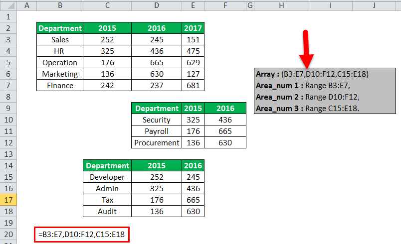
For example, if Reference describes the cells (A1:B4,D1:E4,G1:H4), area_num 1 is the range A1:B4, area_num 2 is the range D1:E4, and area_num 3 is the range G1:H4.
Remarks
-
After reference and area_num have selected a particular range, row_num and column_num select a particular cell: row_num 1 is the first row in the range, column_num 1 is the first column, and so on. The reference returned by INDEX is the intersection of row_num and column_num.
-
If you set row_num or column_num to 0 (zero), INDEX returns the reference for the entire column or row, respectively.
-
row_num, column_num, and area_num must point to a cell within reference; otherwise, INDEX returns a #REF! error. If row_num and column_num are omitted, INDEX returns the area in reference specified by area_num.
-
The result of the INDEX function is a reference and is interpreted as such by other formulas. Depending on the formula, the return value of INDEX may be used as a reference or as a value. For example, the formula CELL(«width»,INDEX(A1:B2,1,2)) is equivalent to CELL(«width»,B1). The CELL function uses the return value of INDEX as a cell reference. On the other hand, a formula such as 2*INDEX(A1:B2,1,2) translates the return value of INDEX into the number in cell B1.
Examples
Copy the example data in the following table, and paste it in cell A1 of a new Excel worksheet. For formulas to show results, select them, press F2, and then press Enter.
|
Fruit |
Price |
Count |
|---|---|---|
|
Apples |
$0.69 |
40 |
|
Bananas |
$0.34 |
38 |
|
Lemons |
$0.55 |
15 |
|
Oranges |
$0.25 |
25 |
|
Pears |
$0.59 |
40 |
|
Almonds |
$2.80 |
10 |
|
Cashews |
$3.55 |
16 |
|
Peanuts |
$1.25 |
20 |
|
Walnuts |
$1.75 |
12 |
|
Formula |
Description |
Result |
|
=INDEX(A2:C6, 2, 3) |
The intersection of the second row and third column in the range A2:C6, which is the contents of cell C3. |
38 |
|
=INDEX((A1:C6, A8:C11), 2, 2, 2) |
The intersection of the second row and second column in the second area of A8:C11, which is the contents of cell B9. |
1.25 |
|
=SUM(INDEX(A1:C11, 0, 3, 1)) |
The sum of the third column in the first area of the range A1:C11, which is the sum of C1:C11. |
216 |
|
=SUM(B2:INDEX(A2:C6, 5, 2)) |
The sum of the range starting at B2, and ending at the intersection of the fifth row and the second column of the range A2:A6, which is the sum of B2:B6. |
2.42 |
Top of Page
See Also
VLOOKUP function
MATCH function
INDIRECT function
Guidelines and examples of array formulas
Lookup and reference functions (reference)
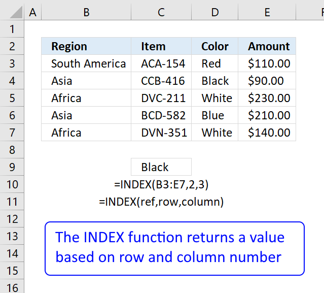
The INDEX function returns the value at a given location in a range or array. INDEX is a powerful and versatile function. You can use INDEX to retrieve individual values, or entire rows and columns. INDEX is frequently used together with the MATCH function. In this scenario, the MATCH function locates and feeds a position to the INDEX function, and INDEX returns the value at that position.
In the most common usage, INDEX takes three arguments: array, row_num, and col_num. Array is the range or array from which to retrieve values. Row_num is the row number from which to retrieve a value, and col_num is the column number at which to retrieve a value. Col_num is optional and not needed when array is one-dimensional.
In the example shown above, the goal is to get the diameter of the planet Jupiter. Because Jupiter is the fifth planet in the list, and Diameter is the third column, the formula in G7 is:
=INDEX(B5:E13,5,3) // diameter of Jupiter
The formula above is of limited value because the row number and column number have been hard-coded. Typically, the MATCH function would be used inside INDEX to provide these numbers. For a detailed explanation with many examples, see: How to use INDEX and MATCH.
Basic usage
INDEX gets a value at a given location in a range of cells based on numeric position. When the range is one-dimensional, you only need to supply a row number. When the range is two-dimensional, you’ll need to supply both the row and column number. For example, to get the third item from the one-dimensional range A1:A5:
=INDEX(A1:A5,3) // returns value in A3
The formulas below show how INDEX can be used to get a value from a two-dimensional range:
=INDEX(A1:B5,2,2) // returns value in B2
=INDEX(A1:B5,3,1) // returns value in A3
INDEX and MATCH
In the examples above, the position is «hardcoded». Typically, the MATCH function is used to find positions for INDEX. For example, in the screen below, the MATCH function is used to locate «Mars» (G6) in row 3 and feed that position to INDEX. The formula in G7 is:
=INDEX(B5:E13,MATCH(G6,B5:B13,0),3)

MATCH provides the row number (4) to INDEX. The column number is still hardcoded as 3.
INDEX and MATCH with horizontal table
In the screen below, the table above has been transposed horizontally. The MATCH function returns the column number (4) and the row number is hardcoded as 2. The formula in C10 is:
=INDEX(C4:K6,2,MATCH(C9,C4:K4,0))

For a detailed explanation with many examples, see: How to use INDEX and MATCH
Entire row / column
INDEX can be used to return entire columns or rows like this:
=INDEX(range,0,n) // entire column
=INDEX(range,n,0) // entire row
where n represents the number of the column or row to return. This example shows a practical application of this idea.
Reference as result
It’s important to note that the INDEX function returns a reference as a result. For example, in the following formula, INDEX returns A2:
=INDEX(A1:A5,2) // returns A2
In a typical formula, you’ll see the value in cell A2 as the result, so it’s not obvious that INDEX is returning a reference. However, this is a useful feature in formulas like this one, which uses INDEX to create a dynamic named range. You can use the CELL function to report the reference returned by INDEX.
Two forms
The INDEX function has two forms: array and reference. Both forms have the same behavior – INDEX returns a reference in an array based on a given row and column location. The difference is that the reference form of INDEX allows more than one array, along with an optional argument to select which array should be used. Most formulas use the array form of INDEX, but both forms are discussed below.
Array form
In the array form of INDEX, the first parameter is an array, which is supplied as a range of cells or an array constant. The syntax for the array form of INDEX is:
INDEX(array,row_num,[col_num])
- If both row_num and col_num are supplied, INDEX returns the value in the cell at the intersection of row_num and col_num.
- If row_num is set to zero, INDEX returns an array of values for an entire column. To use these array values, you can enter the INDEX function as an array formula in horizontal range, or feed the array into another function.
- If col_num is set to zero, INDEX returns an array of values for an entire row. To use these array values, you can enter the INDEX function as an array formula in vertical range, or feed the array into another function.
Reference form
In the reference form of INDEX, the first parameter is a reference to one or more ranges, and a fourth optional argument, area_num, is provided to select the appropriate range. The syntax for the reference form of INDEX is:
INDEX(reference,row_num,[col_num],[area_num])
Just like the array form of INDEX, the reference form of INDEX returns the reference of the cell at the intersection row_num and col_num. The difference is that the reference argument contains more than one range, and area_num selects which range should be used. The area_num is argument is supplied as a number that acts like a numeric index. The first array inside reference is 1, the second array is 2, and so on.
For example, in the formula below, area_num is supplied as 2, which refers to the range A7:C10:
=INDEX((A1:C5,A7:C10),1,3,2)
In the above formula, INDEX will return the value at row 1 and column 3 of A7:C10.
- Multiple ranges in reference are separated by commas and enclosed in parentheses.
- All ranges must on one sheet or INDEX will return a #VALUE error. Use the CHOOSE function as a workaround.
OFFSET is probably the function you want.
=OFFSET(A1:A4,1,,2)
But to answer your question, INDEX can indeed be used to return an array. Or rather, two INDEX functions with a colon between them:
=INDEX(A1:A4,2):INDEX(A1:A4,3)
This is because INDEX actually returns a cell reference OR a number, and Excel determines which of these you want depending on the context in which you are asking. If you put a colon in the middle of two INDEX functions, Excel says «Hey a colon…normally there is a cell reference on each side of one of these» and so interprets the INDEX as just that. You can read more on this at http://www.excelhero.com/blog/2011/03/the-imposing-index.html
I actually prefer INDEX to OFFSET because OFFSET is volatile, meaning it constantly recalculates at the drop of a hat, and then forces any formulas downstream of it to do the same. For more on this, read my post https://chandoo.org/wp/2014/03/03/handle-volatile-functions-like-they-are-dynamite/
You can actually use just one INDEX and return an array, but it’s complicated, and requires something called dereferencing. Here’s some content from a book I’m writing on this:
The worksheet in this screenshot has a named range called Data assigned to the range A2:E2 across the top. That range contains the numbers 10, 20, 30, 40, and 50. And it also has a named range called Elements assigned to the range A5:B5. That Elements range tells the formula in A8:B8 which of those five numbers from the Data range to display.

If you look at the formula in A8:B8, you’ll see that it’s an array-entered INDEX function: {=INDEX(Data,Elements)}. This formula says, “Go to the data range and fetch elements from it based on whatever elements the user has chosen in the Elements range.”
In this particular case, the user has requested the fifth and second items from it. And sure enough, that’s just what INDEX fetches into cells A8:B8: the corresponding values of 50 and 20.
But look at what happens if you take that perfectly good INDEX function and try to put a SUM around it, as shown in A11. You get an incorrect result: 50+20 does not equal 50. What happened to 20, Excel?
For some reason, while =INDEX(Data,Elements) will quite happily fetch disparate elements from somewhere and then return those numbers separately to a range, it is rather reluctant to comply if you ask it to instead give those numbers to another function. It’s so reluctant, in fact, that it passes only the first element to the function.
Consequently, you’re seemingly forced to return the results of the =INDEX(Data,Elements) function to the grid first if you want to do something else with it. Tedious. But pretty much every Excel pro would simply tell you that there’s no workaround…that’s just the way it is, and you have no other choice.
Buuuuuuuut, they’re wrong. At the post http://excelxor.com/2014/09/05/index-returning-an-array-of-values/, mysterious formula superhero XOR outlines two fairly simple ways to “de-reference” INDEX so that you can then use its results directly in other formulas; one of those methods is shown in A18 above. It turns out that if you amend the INDEX function slightly by adding an extra bit to encase that Elements argument, INDEX plays ball. And all you need to do is encase that Elements argument as I’ve done below:
N(IF({1},Elements))
With this in mind, your original misbehaving formula:
=SUM(INDEX(Data,Elements))
…becomes this complex but well-mannered darling:
=SUM(INDEX(Data, N(IF({1},Elements))))
Excel INDEX Function (Examples + Video)
When to use Excel INDEX Function
Excel INDEX function can be used when you want to fetch the value from a tabular data and you have the row number and column number of the data point. For example, in the example below, you can use the INDEX function to get the marks of ‘Tom’ in Physics when you know the row number and the column number in the data set.
What it Returns
It returns the value from a table for the specified row number and column number.
Syntax
=INDEX (array, row_num, [col_num])
=INDEX (array, row_num, [col_num], [area_num])
INDEX function has 2 syntax. The first one is used in most cases, however, in case of three-way lookups, the second one is used (covered in Example 5).
Input Arguments
- array – a range of cells or an array constant.
- row_num – the row number from which the value is to be fetched.
- [col_num] – the column number from which the value is to be fetched. Although this is an optional argument, but if row_num is not provided, it needs to be given.
- [area_num] – (Optional) If array argument is made up of multiple ranges, this number would be used to select the reference from all the ranges.
Additional Notes (Boring Stuff.. But Important to Know)
- If the row number or the column number is 0, it returns the values of the entire row or column respectively.
- If INDEX function is used in front of a cell reference (such as A1:) it returns a cell reference instead of a value (see examples below).
- Most widely used along with the MATCH function.
- Unlike VLOOKUP, INDEX function can return a value from the left of the lookup value.
- INDEX function have two forms – Array form and the Reference form
- ‘Array form’ is where you fetch a value based on row and column number from a given table.
- ‘Reference form’ is where there are multiple tables, and you use the area_num argument to select the table and then fetch a value within it using the row and column number (see live example below).
Excel INDEX Function – Examples
Here are six examples of using Excel INDEX Function.
Example 1 – Finding Tom’s Marks in Physics (a two-way lookup)
Suppose you have a dataset as shown below:
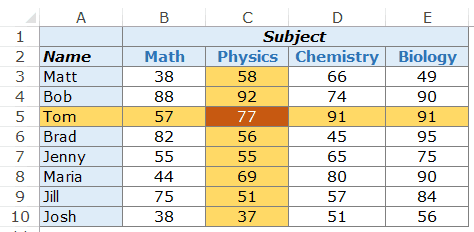
To find Tom’s marks in Physics, use the below formula:
=INDEX($B$3:$E$10,3,2)
This INDEX formula specifies the array as $B$3:$E$10 which has the marks for all the subjects. Then it uses the row number (3) and column number (2) to fetch Tom’s marks in Physics.
Example 2 – Making the LOOKUP Value Dynamic using MATCH Function
It may not always be possible to specify the row number and the column number manually. You may have a huge data set, or you may want to make it dynamic so that it automatically identifies the name and/or subject specified in cells and give the correct result.
Something as shown below:
This can be done using a combination of the INDEX and the MATCH function.
Here is the formula that will make the lookup values dynamic:
=INDEX($B$3:$E$10,MATCH($G$5,$A$3:$A$10,0),MATCH($H$4,$B$2:$E$2,0))
In the above formula, instead of hard-coding the row number and the column number, MATCH function is used to make it dynamic.
- Dynamic Row Number is given by the following part of the formula – MATCH($G$5,$A$3:$A$10,0). It scans the name of students and identifies the lookup value ($G$5 in this case). It then returns the row number of the lookup value in the dataset. For example, if the lookup value is Matt, it’ll return 1, if it is Bob, it’ll return 2 and so on.
- Dynamic Column Number is given by the following part of the formula – MATCH($H$4,$B$2:$E$2,0). It scans the subject names and identifies the lookup value ($H$4 in this case). It then returns the column number of the lookup value in the dataset. For example, if the lookup value is Math, it’ll return 1, if it is Physics, it’ll return 2 and so on.
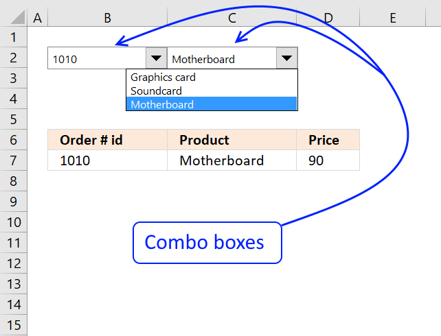
Example 3 – Using Drop Down Lists as Lookup Values
In the above example, we have to manually enter the data. That could be time-consuming and error-prone, especially if you have a huge list of lookup values.
A good idea in such cases is to create a drop down list of the lookup values (in this case, it could be student names and subjects) and then simply choose from the list. Based on the selection, the formula would automatically update the result.
Something as shown below:

This makes a good dashboard component as you can have a huge data set with hundreds of students at the back end, but the end user (let’s say a teacher) can quickly get the marks of a student in a subject by simply making the selections from the drop down.
How to make this:
The formula used in this case is the same used in Example 2.
=INDEX($B$3:$E$10,MATCH($G$5,$A$3:$A$10,0),MATCH($H$4,$B$2:$E$2,0))
The lookup values have been converted into drop-down lists.
Here are the steps to create the Excel drop down list:
- Select the cell in which you want the drop-down list. In this example, in G4, we want the student names.
- Go to Data –> Data Tools –> Data Validation.
- In the Data Validation Dialogue box, within the settings tab, select List from the Allow drop-down.
- In the source, select $A$3:$A$10
- Click OK.
Now you’ll have the drop-down list in cell G5. Similarly, you can create one in H4 for the subjects.
Example 4 – Return Values from an Entire Row/Column
In the above examples, we’ve used Excel INDEX function to do a 2-way lookup and get a single value.
Now, what if you want to get all the marks of a student. This can enable you to find the maximum/minimum score of that student, or the total marks scored in all subjects.
In simple English, you want to first get the entire row of scores for a student (let’s say Bob) and then within those values identify the highest score or the total of all the scores.
Here is the trick.
In Excel INDEX Function, when you enter the column number as 0, it will return the values of that entire row.
So the formula for this would be:
=INDEX($B$3:$E$10,MATCH($G$5,$A$3:$A$10,0),0)
Now this formula. if used as is, would return the #VALUE! error. While it displays the error, in the backend, it returns an array that has all the scores for Tom – {57,77,91,91}.
If you select the formula in the edit mode and press F9, you’ll be able to see the array it returns (as shown below): 
Similarly, based on what the lookup value is, when the column number is specified as 0 (or is left blank), it returns all the values in the row for the lookup value
Now to calculate the total score obtained by Tom, we can simply use the above formula within the SUM function.
=SUM(INDEX($B$3:$E$10,MATCH($G$5,$A$3:$A$10,0),0))
On similar lines, to calculate the highest score, we can use MAX/LARGE and to calculate minimum, we can use MIN/SMALL.

Example 5 – Three Way Lookup Using INDEX/MATCH
Excel INDEX function is built to handle three-way lookups.
What is a three-way lookup?
In the above examples, we’ve used one table with scores for students in different subjects. This is an example of a two-way lookup as we use two variables to fetch the score (student’s name and the subject).
Now, suppose in a year, a student has three different levels of exams, Unit Test, Midterm, and Final Examination (that’s what I had when I was a student).
A three-way lookup would be the ability to get a student’s marks for a specified subject from the specified level of exam. This would make it a three-way lookup as there are three variables (student’s name, subject’s name, and the level of examination).
Here is an example of a three-way lookup:
In the example above, apart from selecting the student’s name and subject name, you can also select the level of exam. Based on the level of exam, it returns the matching value from one of the three tables.
Here is the formula used in cell H4:
=INDEX(($B$3:$E$7,$B$11:$E$15,$B$19:$E$23),MATCH($G$4,$A$3:$A$7,0),MATCH($H$3,$B$2:$E$2,0),IF($H$2="Unit Test",1,IF($H$2="Midterm",2,3)))
Let’s break down this formula to understand how it works.
This formula takes four arguments. INDEX is one of those functions in Excel that has more than one syntax.
=INDEX (array, row_num, [col_num])
=INDEX (array, row_num, [col_num], [area_num])
So far in all the example above, we have used the first syntax, but to do a three-way lookup, we need to use the second syntax.
Now let’s see each part of the formula based on the second syntax.
- array – ($B$3:$E$7,$B$11:$E$15,$B$19:$E$23): Instead of using a single array, in this case, we have used three arrays within parenthesis.
- row_num – MATCH($G$4,$A$3:$A$7,0): MATCH function is used to find the position of the student’s name in cell $G$4 in the list of student’s name.
- col_num – MATCH($H$3,$B$2:$E$2,0): MATCH function is used to find the position of the subject name in cell $H$3 in the list of subject’s name.
- [area_num] – IF($H$2=”Unit Test”,1,IF($H$2=”Midterm”,2,3)): The area number value tells the INDEX function which array to select. In this example, we have three arrays in the first argument. If you select Unit Test from the drop-down, the IF function returns 1 and the INDEX functions select 1st array from the three arrays (which is $B$3:$E$7).
Example 6 – Creating a Reference Using the INDEX Function (Dynamic Named Ranges)
This is one wild use of the Excel INDEX function.
Let’s take a simple example.
I have a list of names as shown below:

Now I can use a simple INDEX function to get the last name on the list.
Here is the formula:
=INDEX($A$2:$A$9,COUNTA($A$2:$A$9))
This function simply counts the number of cells that are not empty and returns the last item from this list (it works only when there are no blanks in the list).
Now, what here comes the magic.
If you put the formula in front of a cell reference, the formula would return a cell reference of the matching value (instead of the value itself).
=A2:INDEX($A$2:$A$9,COUNTA($A$2:$A$9))
You would expect the above formula to return =A2:”Josh” (where Josh is the last value in the list). However, it returns =A2:A9 and hence you get an array of names as shown below:
One practical example where this technique can be helpful is in creating dynamic named ranges.
That’s it in this tutorial. I’ve tried to cover major examples of using the Excel INDEX function. If you would like to see more examples added to this list, let me know in the comments section.
Note: I’ve tried my best to proof read this tutorial, but in case you find any errors or spelling mistakes, please let me know 🙂
Excel INDEX Function – Video Tutorial
Related Excel Functions:
- Excel VLOOKUP Function.
- Excel HLOOKUP Function.
- Excel INDIRECT Function.
- Excel MATCH Function.
- Excel OFFSET Function.
You May Also Like the Following Excel Tutorials:
- VLOOKUP Vs. INDEX/MATCH
- Excel Index Match
- Lookup and Return Values in an Entire Row/Column.
The INDEX function in Excel helps extract the value of a cell, which is within a specified array (range) and, at the intersection of the stated row and column numbers. In other words, the function goes to the cell (within a particular range) whose position is specified, picks its value, and returns it as the output. The INDEX function can also extract an array of values from a dataset.
For example, a worksheet contains the names of continents and the corresponding countries. The entries, typed in Excel (without the double quotation marks), are listed as follows:
Column A
- Cell A1 contains “Asia.”
- Cell A2 contains “Africa.”
- Cell A3 contains “Europe.”
- Cell A4 contains “North America.”
Column B
- Cell B1 contains “India.”
- Cell B2 contains “Nigeria.”
- Cell B3 contains “France.”
- Cell B4 contains “Canada.”
Enter the formula “=INDEX(A1:B4,3,2)” in cell C1. Press the “Enter” key and the output is “France” (without the double quotation marks).
First, the INDEX excel function goes to the range A1:B4. From this range, it fetches the value of the cell, which is at the intersection of the third row (row 3) and the second column (column B). This cell is B3 and its value is “France.”
The INDEX function can return the following values:
- The value at the intersection of the specified row and column numbers
- The value within a table or a named range whose row and column numbers are specified
- The value within non-adjacent ranges whose row and column numbers are specified
The INDEX function in Excel is useful when the dataset is large and one knows the position of the cell from which the value needs to be extracted.
The INDEX function is categorized under the Lookup and Reference functions of Excel.
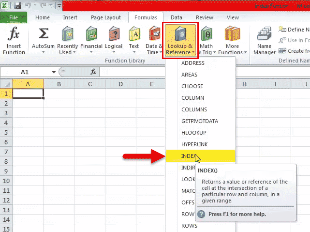
Table of contents
- Index Function in Excel
- Syntax of the INDEX Function in Excel
- How to use the INDEX Function in Excel?
- Example #1–Array Form With a One-Dimensional Array
- Example #2–Array Form With a Two-Dimensional Array
- Example #3–Array Form With Row and/or Column Numbers as Zeros
- Example #4–Reference Form With Multiple Two-Dimensional Arrays
- The Properties Applicable to Both Forms of the INDEX Function
- The INDEX With Other Functions of Excel
- Frequently Asked Questions
- Recommended Articles
Syntax of the INDEX Function in Excel
There are two forms of the INDEX function in excel, the array and the reference. The syntax of both forms is shown in the following image.

Let us discuss both forms of the Excel INDEX function one by one.
The Array Form of the INDEX Excel Function
In the array form, the INDEX function fetches the value of a cell within an array or a table. An array can be either a single range of cells (horizontal or vertical) or multiple adjacent ranges. The value of the cell, which is at the intersection of the supplied row and column numbers, is returned.
The INDEX function accepts the following arguments in the array form:
- Array: This can be a range of cells, table, array constant or named rangeName range in Excel is a name given to a range for the future reference. To name a range, first select the range of data and then insert a table to the range, then put a name to the range from the name box on the left-hand side of the window.read more. The cell whose value is to be returned must necessarily be within this array.
- Row_num: This is the row number of the array from which the value is to be returned.
- Column_num: This is the column number of the array from which the value is to be returned.
The arguments “array” and “row_num” are mandatory, while the argument “column_num” is optional.
It is essential to specify either the “row_num” or the “column_num” to extract a value from a one-dimensional array. To extract a value from a two-dimensional array, one needs to specify both, the “row_num” and the “column_num.”
Note 1: A one-dimensional array consists of a single row or a single column. A two-dimensional array consists of multiple rows and columns.
Note 2: If both “row_num” and “column_num” are entered as zeros (or blanks), the “#VALUE!” error is returned. For instance, the formulas “=INDEX(A1:A4,0,0)” and “=INDEX(A1:A4,,)” return the “#VALUE!” error.
Note 3: If the “array” argument consists of a single column, the “column_num” argument can be omitted, but the “row_num” must be supplied to fetch the value. Likewise, if the “array” argument consists of a single row, the “row_num” argument can be omitted, but the “column_num” must be specified to fetch the value.
For instance, in case of a single column, use the formula “=INDEX(array,row_num)” to fetch a value. In case of a single row, use the formula “=INDEX(array,,column_num)” to fetch a value.
The Reference Form of the INDEX Excel Function
In the reference form, the INDEX function fetches the value of a cell within a defined area (array or range). There can be multiple non-adjacent areas in the reference form. In such cases, the particular area, within which the INDEX function should look for the value, can be specified.
The INDEX function in Excel accepts the following arguments in the reference form:
- Reference: This is the area which can either be a single range or multiple non-adjacent ranges. In the case of multiple non-adjacent ranges, use commas to separate the ranges. In addition, all the ranges must be enclosed within parentheses. For instance, the “reference” argument, (A1:C2, C4:D7) implies two areas (arrays or ranges), A1:C2 and C4:D7.
- Row_num: This is the row number of the area from which the value is to be returned.
- Column_num: This is the column number of the area from which the value is to be returned.
- Area_num: This number indicates the area (of the “reference” argument) in which the INDEX function will look for a value. The first area of the “reference” argument is assigned the number 1. The second area is numbered 2 and so on. For instance, if the “reference” argument is (A1:C2, C4:D7, F4:H8) and the “area_num” is 3, the INDEX function looks for the value in the third area of the “reference” argument, i.e., F4:H8.
The arguments “reference” and “row_num” are required, while the arguments “column_num” and “area_num” are optional.
In the following image, the grey box (pointed by the red arrow) shows the different areas (arrays or ranges) of the reference argument. Further, the area numbers of each range are also given.
Note 1: If the “area_num” argument is omitted, the INDEX excel function looks for the value in the first area of the “reference” argument.
Note 2: All the areas stated in the “reference” argument should be located on one worksheet. If the first area is in one worksheet and the second is in another, the INDEX function returns the “#VALUE!” error.
Note 3: The difference between the array and reference forms is that in the former, adjacent ranges are used, while in the latter, non-adjacent ranges are used.
How to use the INDEX Function in Excel?
Let us consider a few examples to understand the working of the INDEX function in Excel.
You can download this INDEX Function Excel Template here – INDEX Function Excel Template
Example #1–Array Form With a One-Dimensional Array
The following image shows the number of employees (column C) working in the different departments (column B) of an organization.
We want to extract the value of cell C7 with the help of the INDEX function. Use the array form with column C as the single array.
The steps to perform the given task are listed as follows:
Step 1: Enter the following formula in cell E2.
“=INDEX(C3:C7,5)”
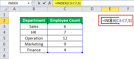
Step 2: Press the “Enter” key. The output in cell E2 is 4.

Explanation: In the formula entered in step 1, we omitted the “column_num” argument since the array (C3:C7) is a single column. Cell C7 is in the fifth row of the array C3:C7. So, the “row_num” argument is entered as 5.
Hence, the given INDEX formula returns 4, which is the value of row 5 of the range C3:C7.
Example #2–Array Form With a Two-Dimensional Array
The following image shows the total number of employees working in five departments of a multinational corporationA multinational company (MNC) is defined as a business entity that operates in its country of origin and also has a branch abroad. The headquarter usually remains in one country, controlling and coordinating all the international branches.
read more (MNC). The numbers pertain to four years, namely, 2015-2018.
We want to extract the value of cell E5 with the help of the INDEX excel function. Use the array form with the entire dataset (except the headings in row 2) as the array.
The steps to perform the given task are listed as follows:
Step 1: Enter the following formula in cell B9.
“=INDEX(B3:F7,3,4)”
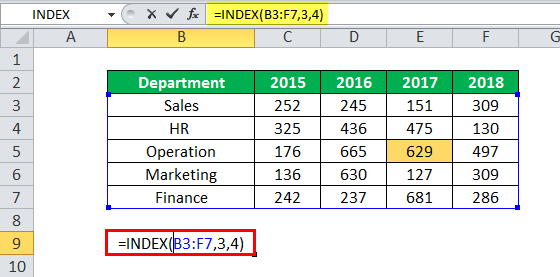
Step 2: Press the “Enter” key. The output in cell B9 is 629.

Explanation: In the preceding formula (entered in step 1), the multiple rows and columns of the dataset are entered as a single array (B3:F7). The INDEX formula returns the value of the cell, which is at the intersection of row 3 and column 4 of the range B3:F7. The cell at this position is cell E5 and its value is 629.
Hence, the output, 629, corresponds to the third row and fourth column of the range B3:F7.
Example #3–Array Form With Row and/or Column Numbers as Zeros
Working on the data of example #2, we want to apply the INDEX function to the entire dataset (B3:F7). Further, observe the output in the following cases:
Case 1: When both arguments “row_num” and “column_num” are zeros
Case 2: When either the “row_num” or the “column_num” is zero
The two cases are discussed as follows:
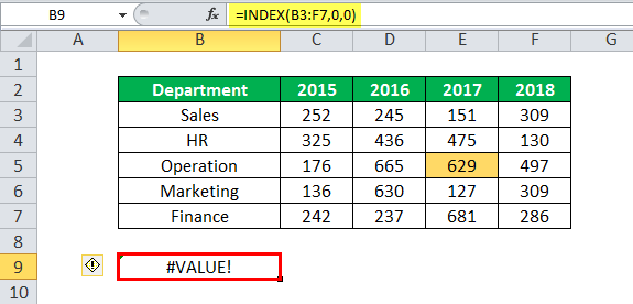
Case 1: When both row and column numbers are entered as zeros, the INDEX function returns the “#VALUE” error.
Steps to be followed: Enter the formula “=INDEX(B3:F7,0,0)” in cell B9. Press the “Enter” key and the output is the “#VALUE” error. This is shown in the following image.
Conclusion: When multiple rows and columns are used as an array, it is necessary to specify both the row and column numbers to extract a particular cell value. In case, both row and column numbers are entered as zeros, the output is the “#VALUE” error.
Case 2: When either the row or the column number is zero, and the INDEX formula is entered as an array formula, the output is an array of values.
Steps to be followed: Select the blank range B11:B15. Enter the formula “=INDEX(B3:F7,0,1)” in the first cell selected (cell B11). Press the keys “Ctrl+Shift+Enter” together.
The outputs in cells B11, B12, B13, B14, and B15 are “Sales,” “HR,” “Operation,” “Marketing,” and “Finance” respectively. All outputs are obtained (without the double quotation marks) the way they are displayed in the range B3:B7.
Alternatively, select the blank row D11:H11. Enter the formula “=INDEX(B3:F7,3,0)” as an array formula. The output is the array of values of row 5 (of the preceding image). So, the output is “Operation,” “176,” “665,” “629,” and “497” without the double quotation marks.
Conclusion: When either the row or column number is specified while the other is set at zero, the INDEX function returns an array of values. However, in such cases, the INDEX formula must be entered as an array formula.
Moreover, it is essential to select a blank output range prior to entering the INDEX formula. This output range should have as many blank cells as the array of the source dataset.
Note: An array formula is usually completed by pressing the CSE keys (Ctrl+Shift+Enter).
Example #4–Reference Form With Multiple Two-Dimensional Arrays
The following image contains three datasets which display the number of employees working in the different departments of an MNC. The first dataset (B2:E7) shows the figures for the years 2015-2017. The second (D9:F12) and third datasets (C14:E18) show the figures for the years 2015 and 2016.
Use the reference form of the INDEX excel function to extract the value of cell F11. Further, categorize the three datasets into three areas which exclude the top row containing the headings.
The steps to perform the preceding tasks are listed as follows:
Step 1: Enter the following formula in cell B20.
“=INDEX((B3:E7,D10:F12,C15:E18),2,3,2)”
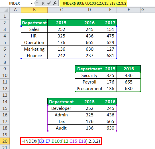
Step 2: Press the “Enter” key. The output is 665, as shown in the following image.

Explanation: In the preceding formula (entered in step 1), the three datasets (given in the question of this example) have been categorized into three areas of the “reference” argument. These areas are B3:E7, D10:F12, and C15:E18. The headings have been excluded from these areas.
Further, the INDEX function looks for a value in the second area (D10:F12). This is because the “area_num” argument is 2. The arguments “row_num” and “column_num” are 2 and 3 respectively. So, the INDEX function returns the value of the cell, which is at the intersection of the second row and the third column in the area D10:F12. This is cell F11.
Hence, the output of the INDEX formula is 665.
The Properties Applicable to Both Forms of the INDEX Function
The properties applicable to both the array and reference forms are listed as follows:
a. If both the arguments “row_num” and “column_num” are entered as zeros, the INDEX excel function returns the “#VALUE!” error.
b. To fetch a value from a single column array, use the following formulas:
- “=INDEX(array,row_num)” in the array form
- “=INDEX((reference),row_num,,area_num)” in the reference form
To fetch a value from a single row array, use the following formulas:
- “=INDEX(array,,column_num)” in the array form
- “=INDEX((reference),,col_num,area_num)” in the reference form
c. If all the column values of an array are required vertically, specify the “column_num” and set the “row_num” at zero. Likewise, if all the row values of an array are required horizontally, specify the “row_num” and set the “column_num” at zero. In both cases, select a blank output range prior to entering the INDEX formula. Moreover, press the keys “Ctrl+Shift+Enter” to complete the formula.
d. The arguments “row_num,” “column_num,” and “area_num” should refer to a cell within the defined array or reference. If not, the INDEX function returns the “#REF!” error.
Note: In pointer “c,” the blank output range can be selected vertically or horizontally depending on whether a vertical or a horizontal array is required.
Further, the number of blank cells (of the output range) must be equal to the cells of the particular row or column array (which is being copied) of the source dataset.
The INDEX With Other Functions of Excel
The INDEX function in excel can be used with several other functions of Excel in the following ways:
a. The INDEX function is used in combination with functions like SUM, AVERAGE, MIN, and MAX to create dynamic ranges. For instance, the formula “AVERAGE(C3:INDEX(C3:C7,3))” returns the average of cells C3, C4, and C5. This is because the formula “INDEX(C3:C7,3)” returns a reference to cell C5. So, the resulting formula becomes “AVERAGE(C3:C5).” Moreover, with a change in the “row_num” argument of the INDEX function, the range of the AVERAGE function changes. This results in a change in the output obtained.
b. The INDEX and MATCH The MATCH function looks for a specific value and returns its relative position in a given range of cells. The output is the first position found for the given value. Being a lookup and reference function, it works for both an exact and approximate match. For example, if the range A11:A15 consists of the numbers 2, 9, 8, 14, 32, the formula “MATCH(8,A11:A15,0)” returns 3. This is because the number 8 is at the third position.
read more functions are used together to perform left lookups. This combination of the INDEX and MATCH functions overcomes the limitations of the VLOOKUP function of Excel. For instance, limitations like compulsory sorting of data, restricted size of the lookup value, decreased speed of Excel, and so on are eliminated.
c. The INDEX function can be used with the COUNTA functionThe COUNTA function is an inbuilt statistical excel function that counts the number of non-blank cells (not empty) in a cell range or the cell reference. For example, cells A1 and A3 contain values but, cell A2 is empty. The formula “=COUNTA(A1,A2,A3)” returns 2.
read more to extract the value of the last used cell of a dataset. With a change in the value of the last used cell, the output updates on its own.
Note 1: Dynamic ranges automatically update with the addition or deletion of data.
Note 2: Usually, the INDEX function returns the value of a cell. However, when a cell referenceCell reference in excel is referring the other cells to a cell to use its values or properties. For instance, if we have data in cell A2 and want to use that in cell A1, use =A2 in cell A1, and this will copy the A2 value in A1.read more and colon (:) precede the INDEX function, it returns a cell reference. This can be observed in the AVERAGE and INDEX formula of pointer “a.”
Frequently Asked Questions
1. Define the INDEX function in Excel.
The INDEX function in Excel returns the value of a cell whose array has been defined. In addition, the row and column numbers of this cell are also specified in the arguments of the INDEX formula.
The INDEX function can also retrieve the values of the entire row or column of a range. The INDEX function has two versions, the array and the reference. Both versions have their own set of arguments.
Note: For details related to the arguments of the INDEX function, refer to the heading “the syntax of the INDEX function in Excel” of this article.
2. How to use the INDEX function in Excel?
The steps for using the INDEX function in Excel are listed as follows:
a. Select the relevant form (array or reference) of the INDEX function to be applied. For this, take into consideration the kind of data.
b. Supply the arguments to the INDEX function. If an array of values is required, select a blank output range prior to entering the arguments.
c. Press either the “Enter” key or the CSE (Ctrl+Shift+Enter) keys, depending on the kind of output required.
The INDEX function processes the arguments. Next, it returns either a single value or an array of values based on the way it has been used.
3. How to use the INDEX MATCH function in place of the VLOOKUP function in Excel?
The INDEX MATCH functions are a versatile combination. This is because these functions can easily lookup a value, regardless of the location of the lookup and the return columns.
The formula to perform a lookup (in rows and columns) by using the INDEX MATCH functions is stated as follows:
“=INDEX(column to return a value from,MATCH(vlookup value,column to be looked up,0),MATCH(hlookup value,row to be looked up,0))”
The working of this formula is explained as follows:
a. The formula “MATCH(vlookup value,column to be looked up,0)” looks for the vlookup value in the column to be looked up (or lookup column). This formula looks for the exact match and returns the row number.
b. The formula “MATCH(hlookup value,row to be looked up,0)” looks for the hlookup value in the row to be looked up (or lookup row). This formula looks for the exact match and returns the column number.
c. The INDEX function uses the row and column numbers returned by the MATCH function. The INDEX function returns a corresponding value from the “column to return a value from” (or return column).
Hence, the INDEX and MATCH formula returns a value at the intersection of certain row and column numbers.
Note 1: It is also possible to supply only the row number or only the column number to the INDEX function. For supplying only the row number, use the first MATCH formula (given in pointer “a”) with the INDEX function. Likewise, to supply only the column number, use the second MATCH formula (given in pointer “b”) with the INDEX function.
Note 2: Looking for a value at the intersection of a row and column is called a 2-way lookup (or 2-dimensional lookup or matrix lookup).
Recommended Articles
This has been a guide to the INDEX function in Excel. Here we discuss the working of the INDEX formula in Excel along with examples and a downloadable Excel template. You may also look at these useful functions in Excel–
- VLOOKUP
- INDIRECT in Excel
- POWER Function in excel
- Hyperlink Excel | Examples
The INDEX function returns a value or the reference to a value from within a table or range. It is used to fetch values from tabular data when you have the row and column numbers of the lookup value.
The INDEX function in Excel has two formats, the Array Format (which is the most basic format), and the Range Format. In this tutorial, you will learn how to use both formats of the INDEX function in Excel.
The Array Format
Syntax
The Array format of the Index function in Excel is used when you want to look up a reference to a cell within a single range. The syntax of the function is:
=INDEX (array, row_num, [col_num], [area_num])
Arguments
array – Required. It is a range of cells, or an array constant. If the array contains only one row or column, the corresponding row_num or col_num argument is optional. If it has more than one row and more than one column, and only row_num or col_num is used, INDEX returns an array of the entire row or column in the array.
row_num – Required. It is the position of the row from which the value is to be fetched. If omitted, col_num is required.
[col_num] – Optional. It is the column position in the reference or array. If omitted, row_num is required.
Returns
The value of an element in a table or an array, selected by the row and column number indexes.
Notes
- If both the row_num and col_num arguments are used, INDEX returns the value in the cell at the intersection of the two.
- If row_num and col_num are both set to 0 (zero), INDEX returns the array of values for the entire column or row, respectively. To use values returned as an array, enter the INDEX function as an array formula in a horizontal range of cells for a row, and in a vertical range of cells for a column. To enter an array formula, press CTRL+SHIFT+ENTER.
The Range Format
Syntax
The Range format of the Index function can be used to extract references from ranges that are made up of more than one area. The syntax of the function is:
INDEX( range, row_num, [col_num], [area_num] )
Arguments
Range – Required. The specified array or range of cells. If multiple areas are inserted directly into the function, the individual areas should be separated by commas and surrounded by brackets (ie. A1:B2, C3:D4, etc).
row_num – Required. It is the row number of the specified area. If set to zero or blank, this defaults to all rows of the specified area within the supplied range.
[col_num] – Optional. Denotes the column number of the specified area. If set to zero or blank, this defaults to all columns of the specified area within the supplied range.
[area_num] – Optional. It is the range in reference that should be used. If this argument is omitted, it defaults to the value 1 (i.e., the reference is taken from the first area in the supplied range.
Returns
Extract references from ranges that are made up of more than one area.
Notes
- After Reference and Area_num have selected a particular range, row_num and col_num select a particular cell: row_num 1 is the first row in the range, col_num 1 is the first column, and so on. The reference returned by INDEX is the intersection of Row_num and Column_num.
- If you set row_num or column_num to 0 (zero), INDEX returns an array of the reference for the entire column or row, respectively.
- row_num, column_num, and area_num must point to a cell within reference; otherwise, INDEX returns the #REF! error. If row_num and col_num are omitted, INDEX returns the area in reference specified by area_num.
- The result of the INDEX function is a reference and is interpreted as such by other formulas. Depending on the formula, the return value of INDEX may be used as a reference or as a value.
Examples
In the following examples, you will learn how to use the array format of the INDEX function.
Using the INDEX Function from the Dialog Box
To enter the INDEX function and arguments using the dialog box for the
example image:
- Click on cell E2, which is the location where the result will be displayed.
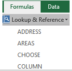
- Click on the Formulas tab of the ribbon menu.
- Choose Lookup and Reference from the ribbon to open the function drop-down list.
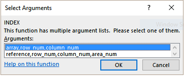
- Click on INDEX in the list to bring up the function’s dialog box.
- In the Select Arguments box, select the option that refers to the array array, row_num, col_num.

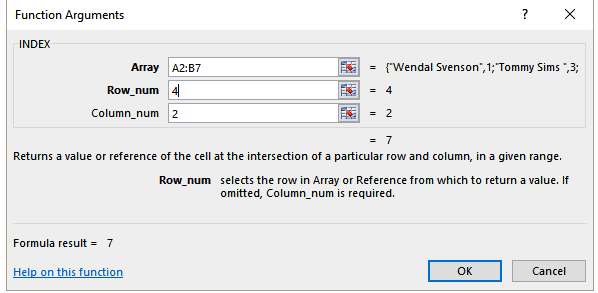
- Highlight cells A2 to A8 in the worksheet to enter the array in the dialog box.
- Click on the row_num line in the dialog box.
- Insert the number 4 where Excel will fetch the value from.
- Click on the col_num line in the dialog box.
- Enter the number 2 on this line to return the value from column 2 which is Years of Experience.
- Click OK to complete the function and close the dialog box.

- The number 7 appears in cell E2 since the employee in row four, Sven Atkins has 7 years of experience.
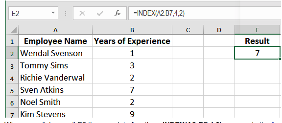
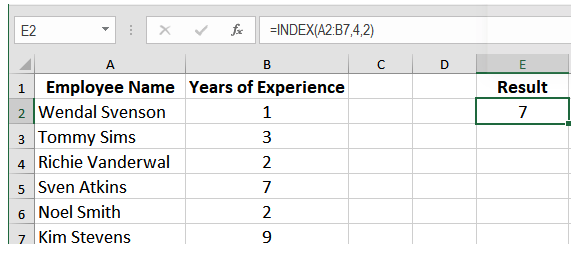
When you click on cell E2 the complete function =INDEX(A2:B7,4,2) appears in the formula bar above the worksheet.
Index Function Excel (Array Format)
In the following example, assign the formula =INDEX(A2:B7,4,2) to cell E2. The Index function returns a reference to row 4 of the range A2:B7, which is cell B5. This has the value 7.
Index Function Excel (Range Format)
In the following example, to find the Production hour of the month Jun, assign the formula =INDEX((C2:D5,D7:E10,F2:G5),3,2,2) to cell G8.
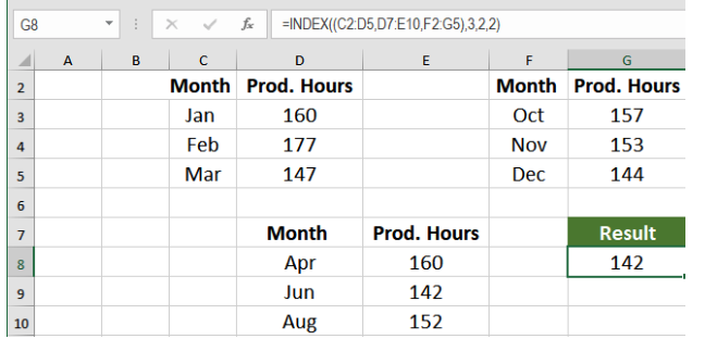
The Index function returns a reference to row 2 and column 2 of the 3rd area in the supplied range. This is cell G8, which evaluates to the value 142.
Still need some help with Excel formatting or have other questions about Excel? Connect with a live Excel expert here for some 1 on 1 help. Your first session is always free.
The INDEX function returns a value from a cell range, you specify which value based on a row and column number.
Formula in cell C9:
=INDEX(B3:E7,2,3)
This formula returns a value from row 2 and column 3 based on cell range B3:E7, note these are relative positions.

The image above shows the relative row and column numbers, row 2 and column 3 are highlighted. The intersection of those two is the value the INDEX function returns.
Video
Table of Contents
- Function Syntax
- Arguments
- How to use an array in INDEX function
- How to use the row_num argument
- Return an array of values — INDEX function
- How to use the [column_num] argument
- How to use the [area_num] argument — INDEX function
- How to return the entire row using the INDEX function
- How to return a column
- How to return a cell range
- How to build a dynamic cell reference using the INDEX function
- Get Excel file
1. Excel Function Syntax
INDEX(array, [row_num], [column_num], [area_num])
Back to top
2. Arguments
| array or cell reference | Required. The cell range you want to get a value from. You can also use an array. |
| [row_num] | Optional. The relative row number of a specific value you want to get. If omitted the INDEX function returns all values if you enter it as an array formula. Update! The 365 subscription version of Excel returns all values without needing to enter the formulas an array formula. |
| [column_num] | Optional. The relative column number of a specific value you want to get. If omitted the INDEX function returns all values if you enter it as an array formula. Update! The 365 subscription version of Excel returns all values without needing to enter the formulas an array formula. |
| [area_num] | Optional. A number representing the relative position of one of the ranges in the first argument. |
Back to top
3. How to use an array in INDEX function
The first argument in the INDEX function is array or a cell reference to a cell range. What is an array? An array is a range of values hardcoded into the formula.
To demonstrate in greater detail what an array is you can convert an array or a cell reference to a group of constants by selecting the cell reference and then press F9 to convert the cell reference to values, see the animated image above.
When you convert a cell range to constants Excel automatically creates double quotes around text values, however, note that numbers are not changed.
B6:D8 becomes {«Staple»,10,10;»Binder»,20,6;»Pen»,30,1} and each value is separated by a delimiting character. Comma (,) is used to separate columns and semicolon (;) to separate rows.
The English language version of excel uses commas and semicolons, other language versions of excel may use other characters. You can change this in the Regional settings in Windows.
Here is an example of an array used in an INDEX function:
=INDEX({«Staple», 10, 10; «Binder», 20, 6; «Pen», 30, 1}, 3, 1)
The greatest disadvantage of using an array is that you need to edit the formula if you need to change one of the values in the array, contrary to a cell reference.
Here is an example of a cell reference being used in an INDEX function:
=INDEX(B6:D8, 3, 1)
You don’t need to edit this formula if one of the values in cell range B6:D8 is changed, the formula is using the new value automatically.
Remember that relative cell references (B6:D8) changes when you copy the cell and paste to cells below. Absolute cell references ($B$6:$D$8) do not change when the cell is copied to cells below.
Read more about converting cell references or formulas: Replace a formula with its result
Back to top
4. How to use the row_num argument
The second argument in the INDEX function is the row_num. It allows you to choose the row in an array or cell range, from which to return a value.
If you use an array or cell range with values distributed in one column only there is no need to use the second optional argument which specifies the column, there is only one column to use. Here is an example of an array containing values in a single column, no comma as a delimiting value in this array which would have indicated that there would have been multiple columns.
=INDEX({«Staple»; «Binder»; «Pen»; «Pencil»; «Eraser»; «Marker»}, 2)
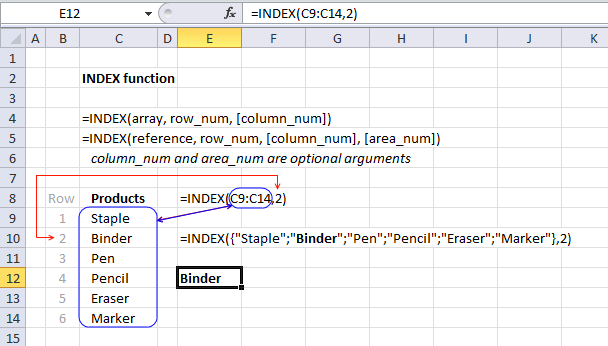
The following formula uses a cell reference instead of hardcoded values:
=INDEX(C9:C14, 2)
Cell range C9:C14 has values separated by a semicolon. The cell range is one-dimensional. In this example, the value from the second row will be returned, see image above.
5. Return an array of values — INDEX function

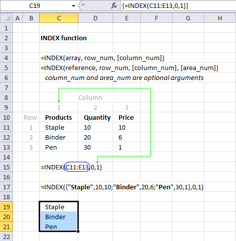
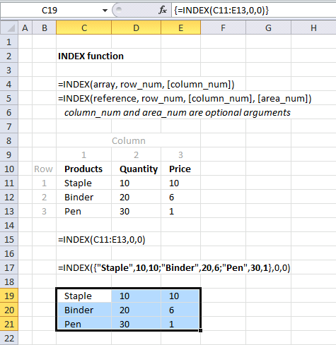
It is also possible to return an array of values if you omit or use a zero as row_num argument:
=INDEX(C9:C14,)
=INDEX(C9:C14,0)
Both these formulas return an array of values. To be able to display all values you need to enter the formula as an array formula in a cell range that has the same number of cells as the cell range or values in the array.
- Select cell range D3:D8.
- Type the formula =INDEX(C9:C14,0)
- Press and hold CTRL + SHIFT simultaneously.
- Press Enter once.
- Release all keys.
The formula in the formula bar changes to {=INDEX(C9:C14,0)}, do not add these curly brackets yourself, they appear automatically. See the image above.
Update 1/22/2020!

Excel users owning Excel 365 subscription version now have the option to not enter the formula as an array formula but as a regular formula. They are called dynamic arrays and behaves differently than array formulas. Array formulas can still be used in order to be compatible with earlier Excel versions, however, Microsoft suggests that you should from now on use dynamic arrays instead of array formulas.
The formula is entered as a regular formula and extends automatically if the cells needed below are empty, this is called spilling by Microsoft. The remaining cells show a greyed out formula in the formula bar, only the first cell contains a formula in black.
The blue border around the cell range indicates that the cell range contains a spilled formula and disappears when you press with left mouse button on a cell outside the range.
Back to top
6. How to use the [column_num] argument
The column_num argument allows you to choose a column from which to return a value. This argument is optional, for example, if you only have values in a single column.
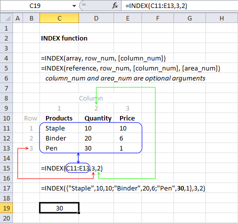
The cell range C11:E13 is two-dimensional meaning there are multiple rows and columns. In this example, the value in the third row and the second column is returned.
=INDEX(C11:E13, 3, 2)
I have greyed out the row and column numbers in the image above, this makes it easier to see that value 30 is where row 3 and column 2 interesects.
The following formula has an array containing constants.
=INDEX({«Staple», 10, 10; «Binder», 20, 6; «Pen», 30, 1}, 3, 2)
{«Staple», 10, 10; «Binder», 20, 6; «Pen», 30, 1} has values separated by commas and semicolons meaning commas separate values between columns and semicolons separate values between rows.
Read more: Looking up data in a cross reference table
Back to top
7. How to use the [area_num] argument — INDEX function
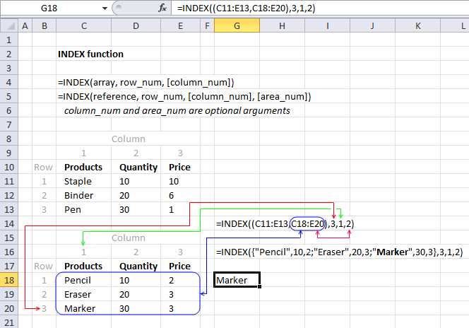
The INDEX function lets you have multiple cell references in the first argument, the area_num argument allows you to pick a cell range in the reference argument.
INDEX(reference, row_num, [column_num], [area_num])
The following formula has two references pointing to two different cell ranges.
=INDEX((C11:E13,C18:E20),3,1,2)
The area_num selects from which cell reference to return a value. In this example, area_num is two therefore the second cell reference is used. The item in the third row and the first column is returned.
Back to top
8. How to return the entire row using the INDEX function
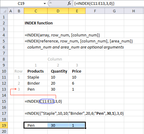
The INDEX function is also capable of returning an array from a column, row, and both columns and rows. The following formula demonstrates how to extract all values from row three:
=INDEX(C11:E13,3,0)
The formula in cell C19:E19 is an array formula.
- Select cell range C19:E19.
- Type =INDEX(C11:E13,3,0) in formula bar.
- Press and hold CTRL + SHIFT simultaeously.
- Press Enter.
- Release all keys.
Back to top
8.1 How to return a column — INDEX function
The example above demonstrates an array formula that returns all values from column 1 from cell range C11:E13.
=INDEX(C11:E13, 0, 1)
Back to top
8.2 How to return a two-dimensional cell range — INDEX function
The example below returns all values from a two-dimensional cell range.
The following array formula returns all values on all rows and columns from a cell range.
=INDEX(C11:E13,0,0)
Back to top
9. How to build a dynamic cell reference using the INDEX function
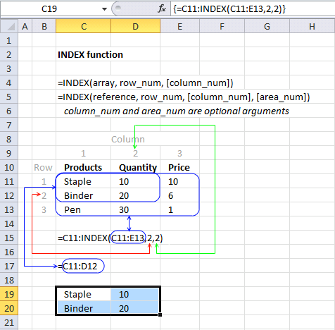
The INDEX function can also be used to create a cell reference, for example, a dynamic range created by a formula in a named range.
Array formula in cell range C19:D20:
=C11:INDEX(C11:E13,2,2)
INDEX(C11:E13,2,2) returns cell reference D12
C11:D12 returns {«Staple»,10;»Binder»,20}
Back to top
Final note
There are some magic things you can do with the array argument. See this post: No more array formulas?
Back to top
10. Excel file
Back to top
‘INDEX‘ function examples
The following 237 articles contain the INDEX function.


Assign records unique random text strings
This article demonstrates a formula that distributes given text strings randomly across records in any given day meaning they may […]
Auto populate a worksheet
Rodney Schmidt asks: I am a convenience store owner that is looking to make a spreadsheet formula. I want this […]
Basic invoice template
Rattan asks: In my workbook I have three worksheets; «Customer», «Vendor» and «Payment». In the Customer sheet I have a […]
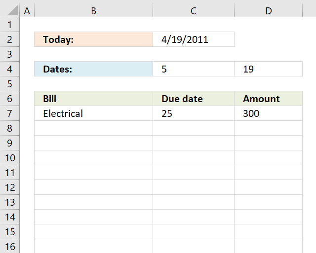
Bill reminder in excel
Brad asks: I’m trying to use your formulas to create my own bill reminder sheet. I envision a workbook where […]
![]()
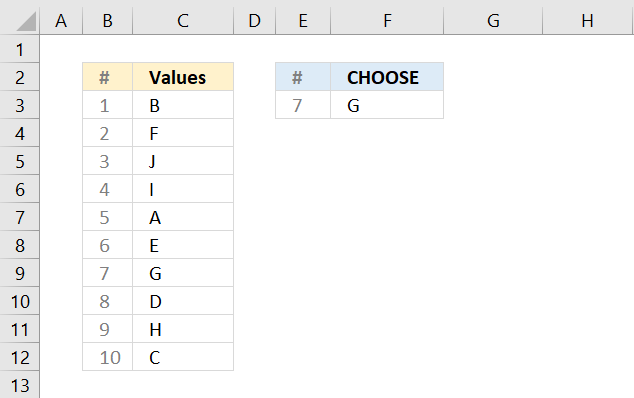
CHOOSE function from list
The picture above shows the CHOOSE function in cell F3, one disadvantage is that you need to press with left […]
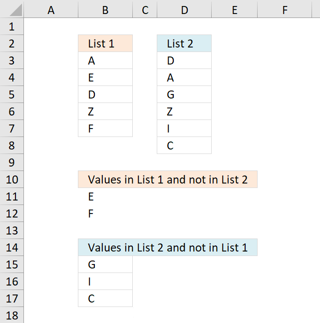
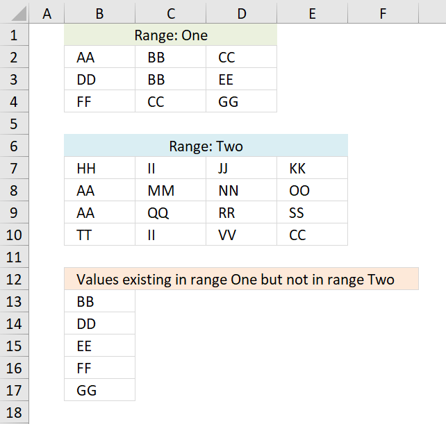
Compare two columns and return differences
This article demonstrates formulas that extract differences between two given lists. The first formula in cell B11 extracts values from […]
Convert column number to column letter
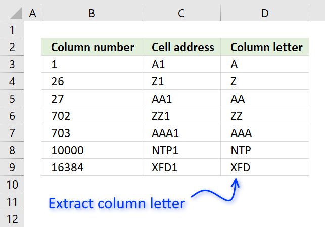
Use the following formula to convert a column number to a column letter: =LEFT(ADDRESS(1, B3, 4), MATCH(B3, {1; 27; 703})) […]
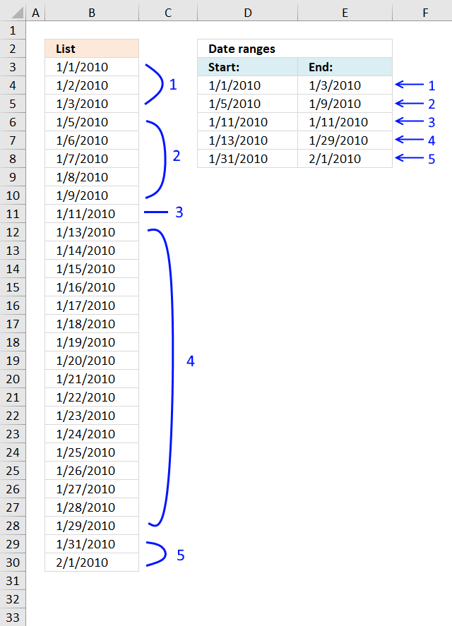
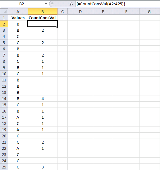
Convert dates into date ranges
The array formula in cell D4 extracts the start dates for date ranges in cell range B3:B30, the array formula […]
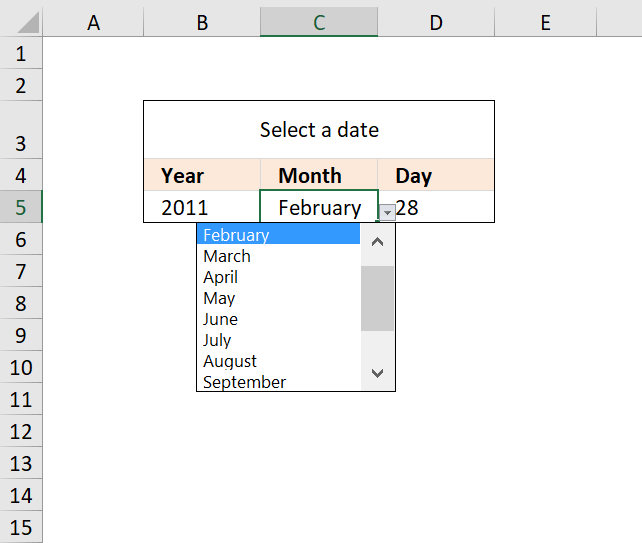
Create a drop down calendar
The drop down calendar in the image above uses a «calculation» sheet and a named range. You can copy the drop-down […]
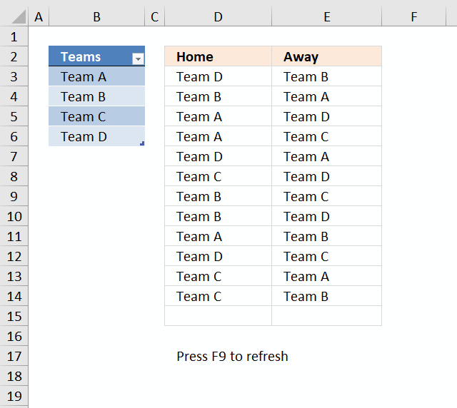
Create a random playlist
This article describes how to create a random playlist based on a given number of teams using an array formula. […]
![]()
Delete blanks and errors in a list
Table of Contents Delete blanks and errors in a list How to find errors in a worksheet 1. Delete blanks […]
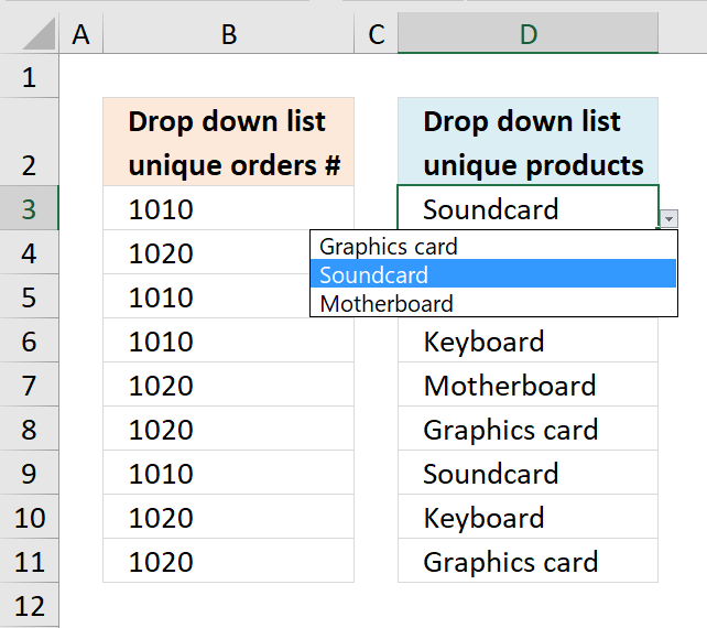
Dependent drop-down lists in multiple rows
This article demonstrates how to set up dependent drop-down lists in multiple cells. The drop-down lists are populated based on […]
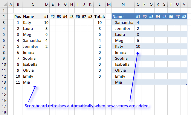
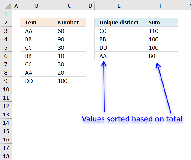
Dynamic scoreboard
This article demonstrates a scoreboard, displayed to the left, that sorts contestants based on total scores and refreshes instantly each […]
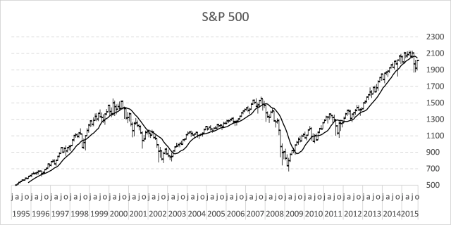
Dynamic stock chart
This stock chart built in Excel allows you to change the date range and the chart is instantly updated. What’s […]
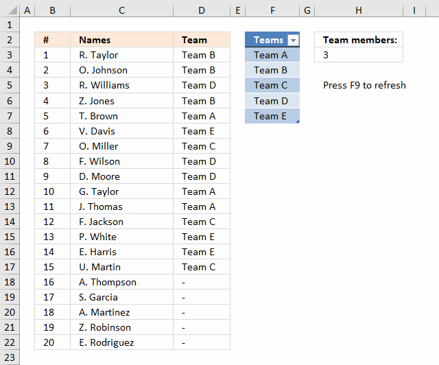
Dynamic team generator
Mark G asks: 1 — I see you could change the formula to have the experssion COUNTIF($C$1:C1, $E$2:$E$5)<5 changed so […]
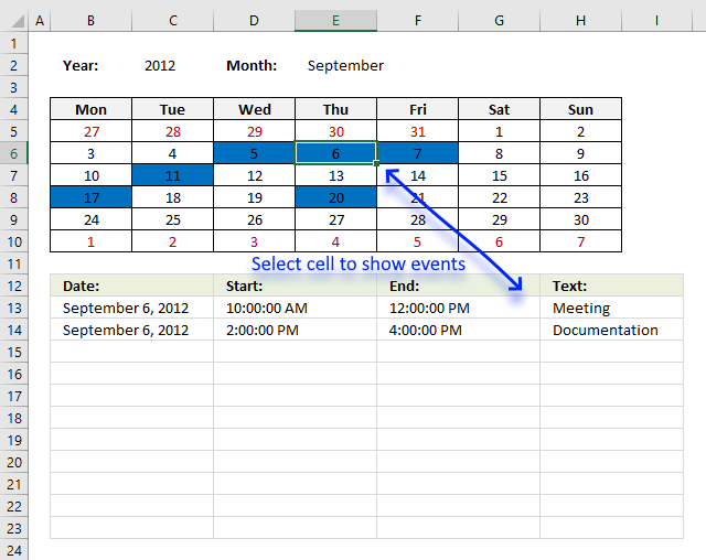
Excel calendar [VBA]
This workbook contains two worksheets, one worksheet shows a calendar and the other worksheet is used to store events. The […]
![]()

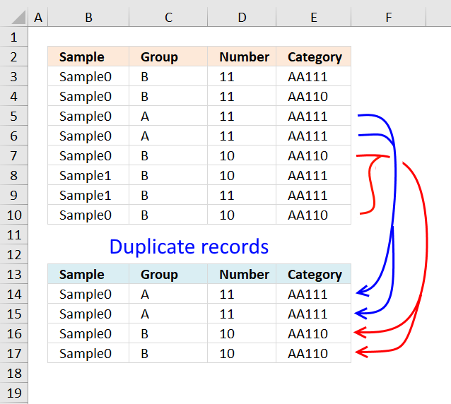
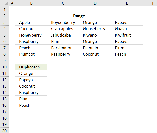
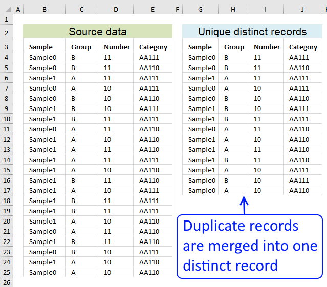
Extract duplicate records
This article describes how to filter duplicate rows with the use of a formula. It is, in fact, an array […]
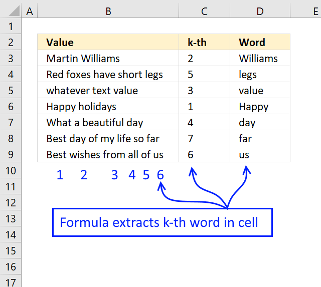
Extract n-th word in cell value
The formula displayed above in cell range D3:D9 extracts a word based on its position in a cell value. For […]
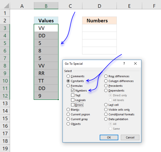
Extract numbers from a column
I this article I will show you how to get numerical values from a cell range manually and using an […]
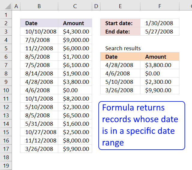
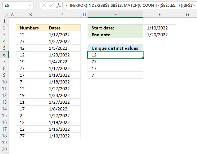
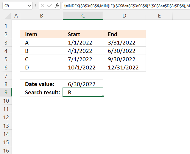
Extract records between two dates
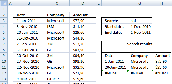
This article presents methods for filtering rows in a dataset based on a start and end date. The image above […]
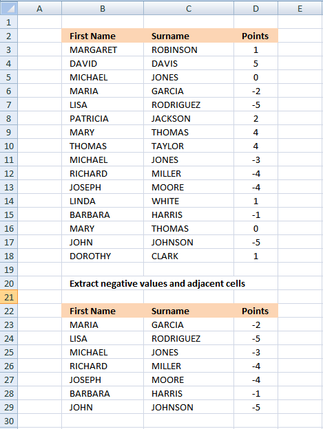
Extract records containing negative numbers
Table of Contents Extract negative values and adjacent cells (array formula) Extract negative values and adjacent cells (Excel Filter) Array […]
![]()
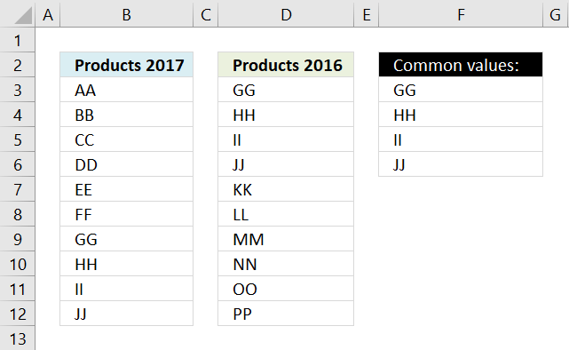
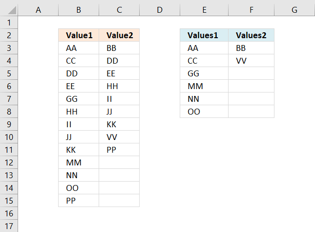
Extract shared values between two columns
This article demonstrates ways to extract shared values in different cell ranges, two and three cell ranges. The Excel 365 […]
![]()
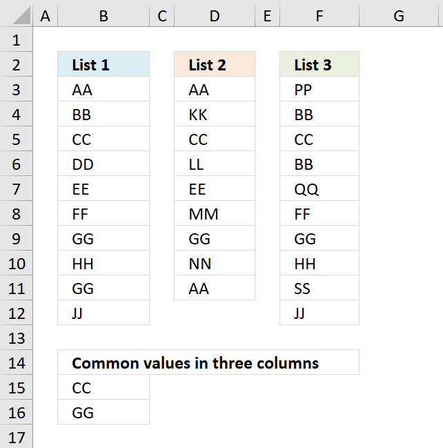
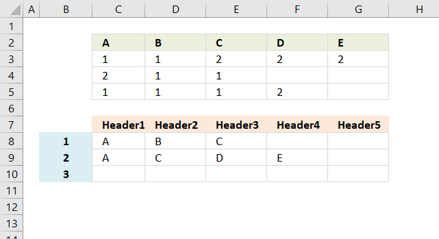
Filter common values from three separate columns
Array formula in B15: =INDEX($B$3:$B$12, MATCH(0, COUNTIF($B$14:B14, $B$3:$B$12)+IF(((COUNTIF($D$3:$D$11, $B$3:$B$12)>0)+(COUNTIF($F$3:$F$12, $B$3:$B$12)>0))=2, 0, 1), 0)) Copy cell B15 and paste it to […]
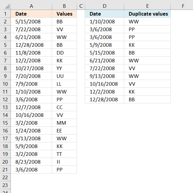
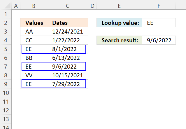
Filter duplicate values and sort by corresponding date
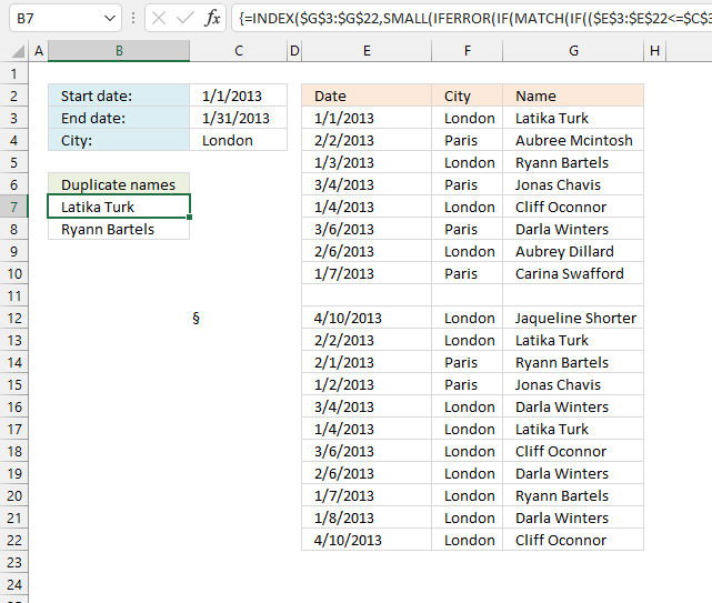
Array formula in D2: =INDEX($A$2:$A$21, MATCH(SMALL(IF(COUNTIF($B$2:$B$21, $B$2:$B$21)>1, COUNTIF($A$2:$A$21, «<«&$A$2:$A$21), «»),ROWS($A$1:A1)), COUNTIF($A$2:$A$21, «<«&$A$2:$A$21), 0)) Array formula in E2: =INDEX($B$2:$B$21, MATCH(SMALL(IF(COUNTIF($B$2:$B$21, $B$2:$B$21)>1, […]
Filter duplicate values based on criteria
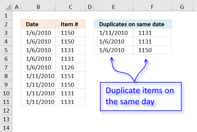
This article demonstrates formulas and Excel tools that extract duplicates based on three conditions. The first and second condition is […]
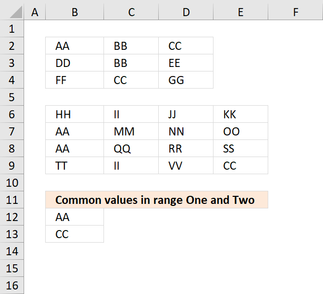
Filter shared records from two tables
I will in this blog post demonstrate a formula that extracts common records (shared records) from two data sets in […]
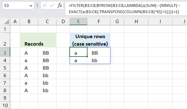
Filter unique distinct records
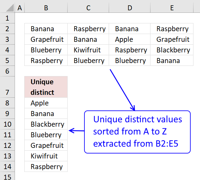
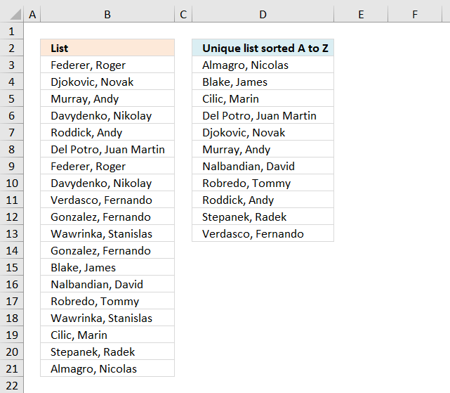
Table of contents Filter unique distinct row records Filter unique distinct row records but not blanks Filter unique distinct row […]
![]()
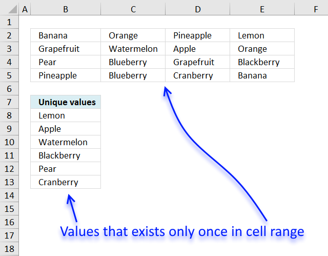
Filter unique values from a cell range
Unique values are values occurring only once in cell range. This is what I am going to demonstrate in this blog […]
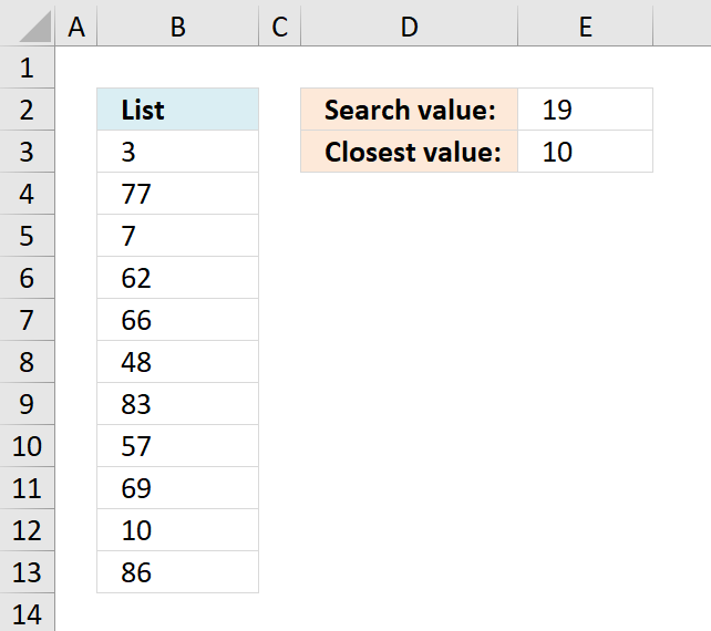
Find closest value
This article demonstrates formulas that extract the nearest number in a cell range to a condition. The image above shows […]
![]()
Find entry based on conditions
Bill Truax asks: Hello Oscar, I am building a spreadsheet for tracking calls for my local fire department. I have a […]
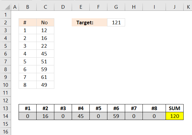
Find numbers closest to sum
Excelxor is such a great website for inspiration, I am really impressed by this post Which numbers add up to […]
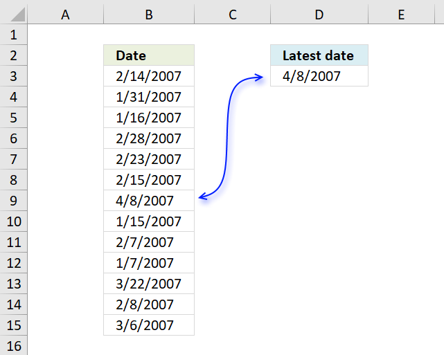
Find the most recent date in a list
The image above shows a formula in cell D3 that extracts the most recent date in cell range B3:B15. =MAX(B3:B15) […]
Free School Schedule Template
This template makes it easy for you to create a weekly school schedule, simply enter the time ranges and the […]
Fuzzy lookups
In this post I will describe a basic user defined function with better search functionality than the array formula in […]
Fuzzy VLOOKUP
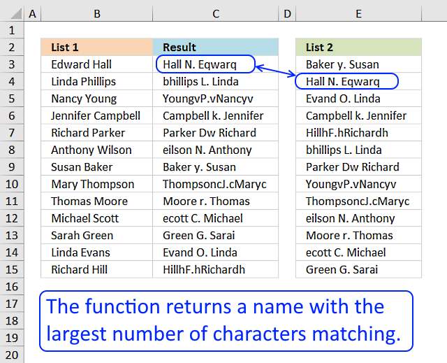
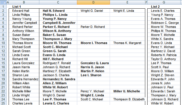
This formula returns multiple values even if they are arranged differently or have minor misspellings compared to the lookup value.
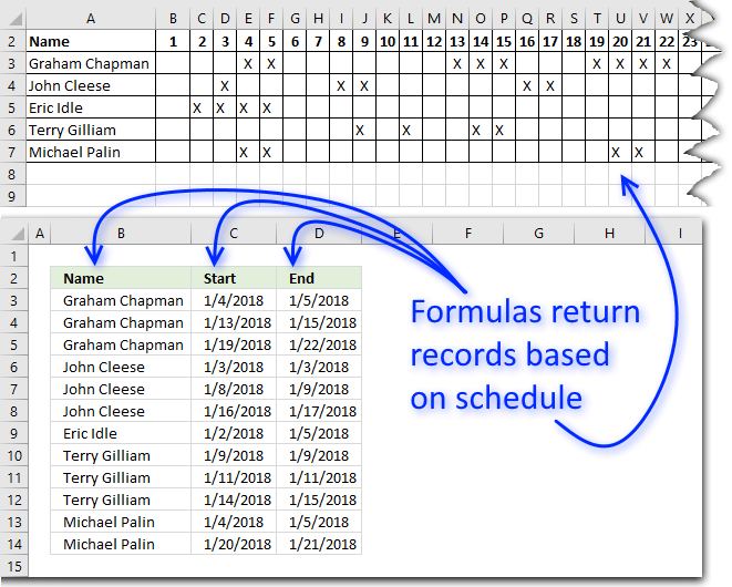
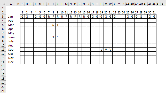
Get date ranges from a schedule
This article demonstrates ways to extract names and corresponding populated date ranges from a schedule using Excel 365 and earlier […]
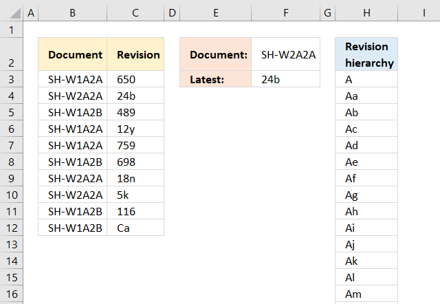
Get the latest revision
Column B contains document names, many of them are duplicates. The adjacent column C has the revision of the documents […]

Highlight lookups in relational tables
This article demonstrates a worksheet that highlights lookups across relational tables. I am using Excel defined Tables, if you add […]
How to animate an Excel chart
This article demonstrates how to create a chart that animates the columns when filtering chart data. The columns change incrementally […]
Functions in this article
Functions in ‘Lookup and reference’ category
The INDEX function function is one of many functions in the ‘Lookup and reference’ category.
Returns the address of a specific cell, you need to provide a row and column number.
Returns the number of cell ranges and single cells in a reference.
Gets a value based on a number.
Returns the column number of the top-left cell of a cell reference.
Calculates the number of columns in a cell range.
Extracts values/rows based on a condition or criteria.
Returns a formula as a text string.
Searches the top row in a data range for a value and return another value on the same column in a row you specify.
Builds a link in a cell.
Returns a value or reference from a cell range or array, you specify which value based on a row and column number.
Returns the cell reference based on a text string and shows the content of that cell reference.
Find a value in a cell range and return a corresponding value on the same row.
Returns the relative position of an item in an array that matches a specified value in a specific order.
Returns a reference to a range that is a given number of rows and columns from a given reference.
Calculates the row number of a cell reference.
Calculate the number of rows in a cell range.
Sorts values from a cell range or array
Sorts a cell range or array based on values in a corresponding range or array.
Downloads stock prices based on a stock quote
Converts a vertical range to a horizontal range, or vice versa.
Returns a unique or unique distinct list.
Lets you search the leftmost column for a value and return another value on the same row in a column you specify.
Search one column for a given value, and return a corresponding value in another column from the same row.
Searches for an item in an array or cell range and returns the relative position.
Excel function categories
Excel functions that let you resize, combine, and shape arrays.
Functions for backward compatibility with earlier Excel versions. Compatibility functions are replaced with newer functions with improved accuracy. Use the new functions if compatibility isn’t required.
Perform basic operations to a database-like structure.
Functions that let you perform calculations to Excel date and time values.
Let’s you manipulate binary numbers, convert values between different numeral systems, and calculate imaginary numbers.
Calculate present value, interest, accumulated interest, principal, accumulated principal, depreciation, payment, price, growth, yield for securities, and other financial calculations.
Functions that let you get information from a cell, formatting, formula, worksheet, workbook, filepath, and other entitites.
Functions that let you return and manipulate logical values, and also control formula calculations based on logical expressions.
These functions let you sort, lookup, get external data like stock quotes, filter values based a condition or criteria, and get the relative position of a given value in a specific cell range. They also let you calculate row, column, and other properties of cell references.
You will find functions in this category that calculates random values, round numerical values, create sequential numbers, trigonometry, and more.
Calculate distributions, binomial distributions, exponential distribution, probabilities, variance, covariance, confidence interval, frequency, geometric mean, standard deviation, average, median, and other statistical metrics.
Functions that let you manipulate text values, substitute strings, find string in value, extract a substring in a string, convert characters to ANSI code among other functions.
Get data from the internet, extract data from an XML string and more.
Excel categories
Latest updated articles.
More than 300 Excel functions with detailed information including syntax, arguments, return values, and examples for most of the functions used in Excel formulas.
More than 1300 formulas organized in subcategories.
Excel Tables simplifies your work with data, adding or removing data, filtering, totals, sorting, enhance readability using cell formatting, cell references, formulas, and more.
Allows you to filter data based on selected value , a given text, or other criteria. It also lets you filter existing data or move filtered values to a new location.
Lets you control what a user can type into a cell. It allows you to specifiy conditions and show a custom message if entered data is not valid.
Lets the user work more efficiently by showing a list that the user can select a value from. This lets you control what is shown in the list and is faster than typing into a cell.
Lets you name one or more cells, this makes it easier to find cells using the Name box, read and understand formulas containing names instead of cell references.
The Excel Solver is a free add-in that uses objective cells, constraints based on formulas on a worksheet to perform what-if analysis and other decision problems like permutations and combinations.
An Excel feature that lets you visualize data in a graph.
Format cells or cell values based a condition or criteria, there a multiple built-in Conditional Formatting tools you can use or use a custom-made conditional formatting formula.
Lets you quickly summarize vast amounts of data in a very user-friendly way. This powerful Excel feature lets you then analyze, organize and categorize important data efficiently.
VBA stands for Visual Basic for Applications and is a computer programming language developed by Microsoft, it allows you to automate time-consuming tasks and create custom functions.
A program or subroutine built in VBA that anyone can create. Use the macro-recorder to quickly create your own VBA macros.
UDF stands for User Defined Functions and is custom built functions anyone can create.
A list of all published articles.

In this article, we will learn How to use the INDEX function in Excel.
Why do we use the INDEX function ?
Given a table of 500 rows and 50 columns and we need to get a value at 455th row and 26th column. For this either we can scroll down to the 455th row and traverse to the 26th column and copy the value. But we can’t treat Excel like hard copies. Index function returns the value at a given row and column index in a table array. Let’s learn the INDEX function Syntax and illustrate how to use the function in Excel below.
INDEX Function in Excel
Index function returns the cell value at matching row and column index in array.
Syntax:
=INDEX(array, row number, [optional column number])
array : It is the range or an array.
row number : Ther row number in your array from which you want to get your value.
column number : [optional] This column number in array. It is optional. If omitted INDEX formula automatically takes 1 as default.
Excel’s INDEX function has two forms known as:
- Array Form INDEX Function
- Reference Form INDEX Function
Example :
All of these might be confusing to understand. Let’s understand how to use the function using an example. Here we have this data.
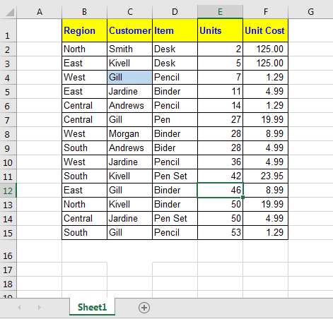
I want to retrieve data at the intersection of 3rd Row and 2nd Column. I write this INDEX formula in cell H2:
The result is Gill:
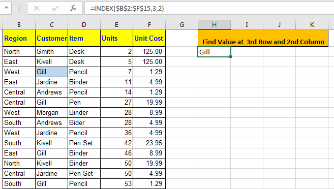
Reference Form INDEX Function
It is much like a multidimensional array index function. Actually in this form of INDEX function, we can give multiple arrays and then in the end we can tell the index from which array to pull data.
Excel INDEX Function Reference Form Syntax
=INDEX( (array1, array2,…), row number, [optional column number], [optional array number] )
(array1, array2,…) : This parenthesis contains a list of arrays. For example (A1:A10,D1:R100,…).
Row number : Ther row number in your array from which you want to get your value.
[optional column number] : This column number in array. It is optional. If omitted, the INDEX formula automatically takes 1 for it.
[optional array number] : The area number from which you want to pull data. In excel it is shown as area_num
Come, let’s have an example.
I have these 3 tables in Excel Worksheet.
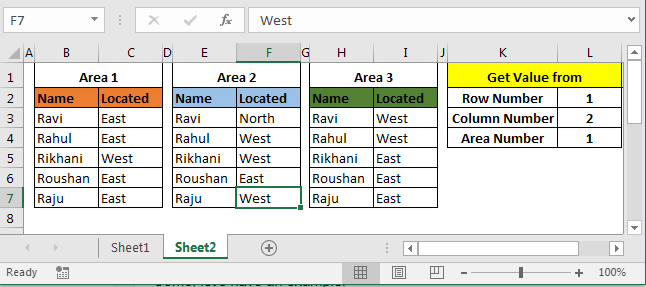
Area 1, Area 2 and Area 3 are my ranges as shown in the above image. I need to retrieve data according to values in cell L2, L3 and L4. So, I write this INDEX formula in cell M1.
=INDEX(($B$3:$C$7,$E$3:$F$7,$H$3:$I$7),L2,L3,L4)
Here L2 is 1, L3 is 2 and L4 is 1. Hence the INDEX function will return the value from the 1st row of the second column from the 1st array. And that is East.
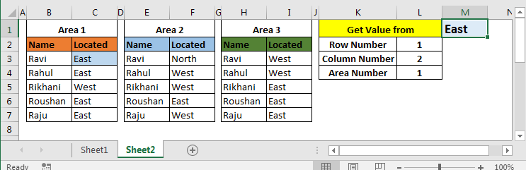
Now change L2 to 2 and L4 to 2. You will have West in M2, as shown in below image.
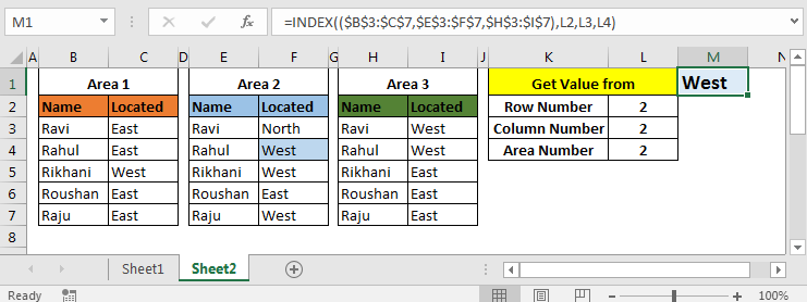
And so on.
The INDEX function in Excel is mostly used with MATCH Function. The INDEX MATCH function is so famous that it is sometimes thought of as one single function. Here I have explained the INDEX MATCH function with multiple criteria in detail. Go check it out. How to lookup values using the INDEX and MATCH function
Hope this article about How to use the INDEX function in Excel is explanatory. Find more articles on calculating values and related Excel formulas here. If you liked our blogs, share it with your friends on Facebook. And also you can follow us on Twitter and Facebook. We would love to hear from you, do let us know how we can improve, complement or innovate our work and make it better for you. Write to us at info@exceltip.com.
Related Articles :
Use INDEX and MATCH to Lookup Value : The INDEX & MATCH formula is used to lookup dynamically and precisely a value in a given table. This is an alternative to the VLOOKUP function and it overcomes the shortcomings of the VLOOKUP function.
Use VLOOKUP from Two or More Lookup Tables : To lookup from multiple tables we can take an IFERROR approach. To lookup from multiple tables, it takes the error as a switch for the next table. Another method can be an If approach.
How to do Case Sensitive Lookup in Excel : The excel’s VLOOKUP function isn’t case sensitive and it will return the first matched value from the list. INDEX-MATCH is no exception but it can be modified to make it case sensitive.
Lookup Frequently Appearing Text with Criteria in Excel : The lookup most frequently appears in text in a range we use the INDEX-MATCH with MODE function.
Popular Articles :
How to use the IF Function in Excel : The IF statement in Excel checks the condition and returns a specific value if the condition is TRUE or returns another specific value if FALSE.
How to use the VLOOKUP Function in Excel : This is one of the most used and popular functions of excel that is used to lookup value from different ranges and sheets.
How to use the SUMIF Function in Excel : This is another dashboard essential function. This helps you sum up values on specific conditions.
How to use the COUNTIF Function in Excel : Count values with conditions using this amazing function. You don’t need to filter your data to count specific values. Countif function is essential to prepare your dashboard.
Skip to content
В этом руководстве вы найдете ряд примеров формул, демонстрирующих наиболее эффективное использование ИНДЕКС в Excel.
Из всех функций Excel, возможности которых часто недооцениваются и используются недостаточно, ИНДЕКС определенно занимает место в первой десятке. Между тем, эта функция умна, гибка и универсальна.
Итак, что такое функция ИНДЕКС в Excel? По сути, формула ИНДЕКС (в английской версии – INDEX) возвращает ссылку на ячейку из заданного массива или диапазона. Другими словами, вы используете её, когда знаете (или можете определить) положение элемента в диапазоне и хотите затем получить значение этого элемента.
- Синтаксис и способы использования
- Получение N-го элемента из списка
- Получение всех значений в строке или столбце
- Использование ИНДЕКС с другими функциями (СУММ, СРЗНАЧ, МАКС, МИН)
- Формула ИНДЕКС для создания динамических диапазонов и раскрывающихся списков
- Мощный поиск с ИНДЕКС/ПОИСКПОЗ
- Формула ИНДЕКС для получения одного диапазона из списка диапазонов
Если вы оцените реальный потенциал функции ИНДЕКС, это может кардинально изменить способы расчета, анализа и представления данных в ваших таблицах.
Функция ИНДЕКС в Excel — синтаксис и основные способы использования
В Excel есть две версии функции ИНДЕКС — форма массива и форма ссылки. Обе их можно использовать во всех версиях Microsoft Excel 365, 2019, 2016, 2013, 2010, 2007 и 2003.
Форма массива ИНДЕКС
В данном случае функция ИНДЕКС возвращает значение элемента в таблице или массиве на основе указанных вами номеров строк и столбцов.
ИНДЕКС(массив,номер_строки,[номер_столбца])
- массив — это диапазон ячеек, именованный диапазон или таблица.
- Номер_строки — это номер строки в массиве, из которого нужно вернуть значение. Если этот аргумент опущен, требуется следующий – номер_столбца.
- Номер_столбца — это номер столбца, из которого нужно вернуть значение. Если он опущен, требуется номер_строки.
Например, формула =ИНДЕКС(C2:F11;4;3) возвращает значение на пересечении четвертой строки и третьего столбца в диапазоне C2:F11, что является значением в ячейке D4.
Чтобы получить представление о том, как формула ИНДЕКС работает с реальными данными, взгляните на следующий пример:

Вместо того, чтобы вводить в формулу номера строк и столбцов, вы можете указать ссылки на ячейки, чтобы получить более универсальную формулу:
=ИНДЕКС(C2:F11;I1;I2)
Итак, эта формула ИНДЕКС возвращает количество товаров точно на пересечении номера товара, указанного в ячейке I1 (номер_строки), и номера недели, введенного в ячейке I2 (номер_столбца).
Примечание. Использование абсолютных ссылок ($C$2:$F$11) вместо относительных ссылок (C2:F11) в аргументе массива упрощает копирование формулы в другие ячейки. Кроме того, вы можете преобразовать диапазон в таблицу (Ctrl + Т) и обращаться к нему по имени таблицы.
Что нужно помнить
- Если аргумент массива состоит только из одной строки или столбца, вы можете указать или не указать соответствующий аргумент номер_строки или номер_столбца.
- Если аргумент массива включает более одной строки, а номер_строки опущен или равен 0, функция ИНДЕКС возвращает массив всего столбца. Точно так же, если массив включает более одного столбца, а аргумент номер_столбца опущен или равен 0, формула ИНДЕКС возвращает всю строку. Вот пример формулы, демонстрирующий такое поведение.
- Аргументы номер_строки и номер_столбца должны ссылаться на ячейку в массиве; в противном случае формула ИНДЕКС вернет ошибку #ССЫЛКА!.
Форма ИНДЕКС в виде ссылки
Ссылочная форма функции ИНДЕКС Excel возвращает ссылку на ячейку на пересечении указанной строки и столбца.
ИНДЕКС(ссылка, номер_строки, [номер_столбца], [номер_области] )
- ссылка — это один или несколько диапазонов.
Если вы вводите более одного диапазона, разделите диапазоны точкой с запятой и заключите аргумент ссылки в круглые скобки, например (A1:B5; D1:F5).
Если каждый диапазон в ссылке содержит только одну строку или столбец, соответствующий аргумент номер_строки или номер_столбца является необязательным.
- номер_строки – порядковый номер строки в диапазоне, из которого возвращается ссылка на ячейку, аналогично форме массива.
- номер_столбца — порядковый номер столбца, из которого возвращается ссылка на ячейку, также работает аналогично форме массива.
- номер_области — необязательный параметр, указывающий, какой диапазон из ссылочного аргумента использовать. Если он не указан, формула ИНДЕКС вернет результат для первого диапазона, указанного в ссылке.
Например, формула =ИНДЕКС((B2:F4;B8:F11);3;2;2) возвращает значение ячейки С10, которая находится на пересечении 3-й строки и 2-го столбца во второй области (B8:F11).

Что нужно помнить о функции ИНДЕКС в форме ссылки
- Если аргумент номер_строки или номер_столбца равен нулю (0), формула ИНДЕКС возвращает ссылку для всего столбца или строки соответственно.
- Если и номер_строки, и номер_столбца опущены, функция ИНДЕКС возвращает область, указанную в аргументе номер_области.
- Все аргументы (номер_строки, номер_столбца и номер_области) должны ссылаться на ячейку в пределах заданного диапазона. В противном случае формула ИНДЕКС вернет ошибку #ССЫЛКА!
Обе формулы ИНДЕКС, которые мы обсуждали до сих пор, очень просты и служат только для иллюстрации. Ваши реальные формулы, вероятно, будут намного сложнее. Поэтому давайте рассмотрим несколько наиболее эффективных способов использования ИНДЕКС в Excel.
Как использовать функцию ИНДЕКС в Excel — примеры формул
Возможно, сама по себе функция ИНДЕКС в Excel не имеет большого практического применения, но в сочетании с другими функциями, такими как ПОИСКПОЗ или СЧËТ, она может создавать очень мощные формулы.
Далее во всех наших формулах ИНДЕКС (кроме последней) мы будем использовать приведенные ниже данные.

1. Получение N-го элемента из списка
Это основное использование функции ИНДЕКС и простейшая её формула. Чтобы получить определенный элемент из списка, вы просто пишете: =ИНДЕКС(диапазон; n), где диапазон — это диапазон ячеек или именованный диапазон, а n — позиция элемента, который вы хотите из него получить.
Чтобы получить значение ячейки на пересечении определенной строки и столбца, вы используете тот же подход с той лишь разницей, что вы указываете и номер строки, и номер столбца. На самом деле, вы уже видели такую формулу в действии, когда мы обсуждали форму массива функции ИНДЕКС .
И вот еще один пример. В нашем образце таблицы, чтобы найти четвертую по величине планету в Солнечной системе, вы сортируете таблицу по столбцу Диаметр и используете следующую формулу ИНДЕКС:
=ИНДЕКС(A5:E13;4;1)
- A5:E13 — это ссылка на диапазон с данными.
- Номер_строки равен 4, потому что вы ищете четвертый элемент в списке,
- Номер_столбца равен 1, потому что мы хотим извлечь имя планеты.
Естественно, вы можете использовать ссылку на ячейку в аргументах номер_строки и/или номер_столбца, чтобы сделать вашу формулу более универсальной, как показано на скриншоте ниже:

Кроме того, вы можете не сортировать таблицу вручную, а сделать это при помощи формулы.
=ИНДЕКС(СОРТ(A5:E13;3;-1);B1;1)
Функция СОРТ сортирует таблицу по третьему столбцу в порядке убывания. Ну а затем ИНДЕКС делает всё остальное.
2. Получение всех значений в строке или столбце
Помимо извлечения одной ячейки, функция ИНДЕКС может возвращать массив значений из всей строки или столбца . Чтобы получить все значения из определенного столбца, вы должны опустить аргумент номер_строки или установить его равным 0. Аналогичным образом, чтобы получить всю строку, вы передаете пустое значение или 0 в номер_столбца.
Такие формулы ИНДЕКС вряд ли можно использовать сами по себе, потому что Excel не может уместить массив значений, возвращаемых формулой, в одну ячейку, и вы получите ошибку #ЗНАЧ!. Однако, если вы используете ИНДЕКС в сочетании с другими функциями, такими как СУММ или СРЗНАЧ, вы получите отличные результаты.
Например, вы можете использовать следующую формулу для расчета средней температуры планет в Солнечной системе:
=СРЗНАЧ(ИНДЕКС(A4:E12;;4))
В приведенной выше формуле аргумент номер_столбца равен 4, потому что температура находится в четвертом столбце нашей таблицы. Параметр номер_строки опущен.

Аналогичным образом можно найти минимальную и максимальную температуры:
=МИН(ИНДЕКС(A4:E12;;4))
=МАКС(ИНДЕКС(A4:E12;;4))
И посчитаем общую массу планет (масса – второй столбец в таблице):
=СУММ(ИНДЕКС(A4:E12;;2))
С практической точки зрения функция ИНДЕКС в приведенной выше формуле лишняя. Вы можете просто написать =СРЗНАЧ(D4:D12) и получить те же результаты.
При работе с реальными данными эта функция может оказаться полезной как часть более сложных формул, которые вы используете для анализа данных.
К примеру, формула =СУММ(ИНДЕКС(A4:E12;;С1)) позволит вам подсчитывать сумму в том столбце, номер которого вы укажете в ячейке C1.
3. Использование ИНДЕКС с другими функциями (СУММ, СРЗНАЧ, МАКС, МИН)
Из предыдущих примеров у вас может сложиться впечатление, что формула ИНДЕКС возвращает значения, но на самом деле она возвращает ссылку на ячейку, содержащую значение. И этот пример демонстрирует, как эту возвращаемую ссылку можно использовать.
Поскольку результат формулы ИНДЕКС является ссылкой, мы можем использовать его в других функциях для создания динамического диапазона. Звучит запутанно? Сейчас поясним.
Предположим, у вас есть формула =СРЗНАЧ(D4:D12), которая возвращает среднее значений в ячейках D4:D12. Вместо того, чтобы писать диапазон непосредственно в формуле, вы можете заменить либо D4, либо D12, либо их оба, функцией ИНДЕКС, например:
=СРЗНАЧ(D4 : ИНДЕКС(D1:D20,12))
Обе приведенные выше формулы дадут один и тот же результат, поскольку функция ИНДЕКС также возвращает ссылку на ячейку В12 (номер строки равен 12, номер столбца опущен). Разница в том, что диапазон формулы СРЗНАЧ / ИНДЕКС является динамическим, и как только вы измените аргумент номер_строки в ИНДЕКС, то диапазон, обрабатываемый функцией СРЗНАЧ, также изменится, и формула вернет другой результат.
По-видимому, такое использование формулы ИНДЕКС кажется слишком сложным и не всегда рациональным и логичным. Но этот подход имеет важное практическое применение, как показано в следующих примерах.
Пример 1. Вычислить среднее значение первых N элементов в списке
Допустим, вы хотите узнать средний диаметр N самых больших планет в солнечной системе.
Количество позиций, которые мы будем использовать для расчета, указываем в ячейке В1.
Затем вы сортируете таблицу по столбцу диаметра от наибольшего к наименьшему и используете следующую формулу расчёта среднего значения:
=СРЗНАЧ(C5:ИНДЕКС(C5:C13;B1))

Как видите, количество значений для расчета среднего мы можем выбирать, не корректируя саму формулу
Пример 2. Сумма элементов между указанными двумя элементами
Если вы хотите определить элементы верхней и нижней границы в своей формуле, вам просто нужно использовать две функции ИНДЕКС, чтобы вернуть первый и последний элемент, которые вам нужны.
Например, следующая формула при помощи функции СУММ возвращает сумму значений в столбце Масса между двумя элементами, указанными в ячейках B1 и Е1:
=СУММ(ИНДЕКС(B5:B13;B1):ИНДЕКС(B5:B13;E1))

4. Формула ИНДЕКС для создания динамических диапазонов и раскрывающихся списков
Как это часто бывает, когда вы начинаете упорядочивать данные на листе, вы можете не знать, сколько записей у вас в конечном итоге будет. Это не относится к нашей таблице планет, которая кажется полной, но кто знает…
В любом случае, если у вас есть изменяющееся количество элементов в данном столбце, скажем, от A1 до An , вы можете создать динамический именованный диапазон , включающий все ячейки с данными. При этом вы хотите, чтобы диапазон корректировался автоматически по мере добавления новых элементов или удаления некоторых из существующих. Например, если у вас сейчас 10 элементов, ваш именованный диапазон будет A1:A10. Если вы добавите новую запись, именованный диапазон автоматически расширится до A1:A11, а если вы передумаете и удалите эти вновь добавленные данные, диапазон автоматически вернется к A1:A10.
Основное преимущество этого подхода заключается в том, что вам не нужно постоянно обновлять все формулы в книге, чтобы убедиться, что они относятся к правильным диапазонам.
Одним из способов определения динамического диапазона является использование функции Excel СМЕЩ :
=СМЕЩ($A$2; 0; 0; СЧЁТЗ($A1:$A100)-1; 1)
Другим возможным решением является использование ИНДЕКС Excel вместе с СЧËТЗ:
=$A$2:ИНДЕКС($A2:$A100; СЧЁТЗ($A2:$A100))
В обеих формулах A2 — это ячейка, содержащая первый элемент списка. Динамический диапазон, создаваемый обеими формулами, будет идентичным.
Разница заключается в подходах. В то время как функция СМЕЩ перемещается от начальной точки на определенное количество строк и/или столбцов, то ИНДЕКС находит ячейку на пересечении определенной строки и столбца. Функция СЧËТЗ, используемая в обеих формулах, получает количество непустых ячеек в интересующем нас столбце.
В этом примере в столбце A 9 непустых ячеек, поэтому СЧËТЗ возвращает 9. Следовательно, ИНДЕКС возвращает $A$9, то есть последнюю использованную ячейку в столбце A (обычно ИНДЕКС возвращает значение, но в этой формуле оператор ссылки (:) заставляет его вернуть ссылку). И поскольку $A$1 является нашей отправной точкой, конечным результатом формулы будет диапазон $A$1:$A$9.
На следующем рисунке показано, как можно использовать такую формулу ИНДЕКС для создания динамического выпадающего списка.

Примечание. Самый простой способ создать динамически обновляемый выпадающий список — сделать именованный список на основе таблицы Excel. В этом случае вам не понадобятся сложные формулы, поскольку таблицы Excel сами по себе являются динамическими диапазонами.
Вы также можете использовать функцию ИНДЕКС для создания зависимых раскрывающихся списков, и в следующем руководстве объясняются все необходимые шаги: Создание каскадного раскрывающегося списка в Excel .
5. Мощный поиск с ИНДЕКС/ПОИСКПОЗ
Выполнение вертикального поиска — вот где функция ИНДЕКС действительно великолепна. Если вы когда-либо пробовали использовать функцию ВПР Excel , вы хорошо знаете ее многочисленные ограничения, такие как невозможность извлечения значений из столбцов слева от столбца поиска или ограничение в 255 символов для значения поиска.
Связка ИНДЕКС/ПОИСКПОЗ во многих отношениях превосходит ВПР:
- Никаких проблем с «левым» ВПР.
- Нет ограничений на размер искомого значения.
- Сортировка не требуется (ВПР с приблизительным совпадением требует сортировки столбца подстановки в порядке возрастания).
- Вы можете вставлять и удалять столбцы в таблице, не обновляя каждую связанную формулу.
- И последнее, но не менее важное: ИНДЕКС/ПОИСКПОЗ не замедляет работу Excel, как это происходит, если использовать несколько формул ВПР в большой таблице.
Вы используете ИНДЕКС / ПОИСКПОЗ следующим образом:
=ИНДЕКС ( столбец для возврата значения , (ПОИСКПОЗ ( искомое значение , столбец для поиска , 0))
Например, по коду заказа мы можем найти название товара. При этом функция ПОИСКПОЗ ищет совпадение с кодами заказа, а затем передает номер найденной позиции в функцию ИНДЕКС. Та же в свою очередь извлекает соответствующее значение из переданного ей диапазона.

Таким образом организуется так называемый «левый» поиск, когда нужно извлечь значение из столбца, находящегося слева от столбца поиска. Функция ВПР сделать это не может. Более подробно о «левом» поиске читайте в этой статье.
Дополнительные советы и примеры формул см. в руководстве по Excel ИНДЕКС/ПОИСКПОЗ .
6. Формула ИНДЕКС для получения одного диапазона из списка диапазонов
Еще одно умное и эффективное использование функции ИНДЕКС в Excel — это возможность получить один диапазон из списка диапазонов.
Предположим, у вас есть несколько списков (например, сведения о еженедельных продажах). Вы можете рассчитать среднее значение или суммировать значения в любом выбранном диапазоне с помощью одной формулы.
Вы можете использовать следующую формулу индекса для расчета суммы продаж в выбранном диапазоне:
=СУММ(ИНДЕКС((C2:C11;D2:D11;E2:E11;F2:F11);;;I1))
Обратите внимание, что сейчас мы используем функцию ИНДЕКС в виде ссылки. Число в последнем аргументе (номер_области) сообщает формуле, какой именно диапазон выбрать.
На скриншоте ниже для номера диапазона (ячейка I1) установлено значение 2. Поэтому формула вычисляет сумму продаж за вторую неделю. Выбран второй по счёту диапазон в списке – D2:D11.

Чтобы сделать формулу еще более удобной для пользователя, вы можете использовать проверку данных и создать в ячейке I2 выпадающий список с номерами недель, чтобы предотвратить ошибки и опечатки:

Вот несколько основных способов применения формулы ИНДЕКС в Excel.
Я надеюсь, что эти примеры показали вам, как использовать потенциал функции ИНДЕКС в ваших рабочих листах. Спасибо за чтение!