Индексы ячеек excel vba

Обращение к ячейке на листе Excel из кода VBA по адресу, индексу и имени. Чтение информации из ячейки. Очистка значения ячейки. Метод ClearContents объекта Range.

Обращение к ячейке по адресу

Допустим, у нас есть два открытых файла: «Книга1» и «Книга2», причем, файл «Книга1» активен и в нем находится исполняемый код VBA.

В общем случае при обращении к ячейке неактивной рабочей книги «Книга2» из кода файла «Книга1» прописывается полный путь:

Workbooks(«Книга2.xlsm»).Sheets(«Лист2»).Range(«C5») Workbooks(«Книга2.xlsm»).Sheets(«Лист2»).Cells(5, 3) Workbooks(«Книга2.xlsm»).Sheets(«Лист2»).Cells(5, «C») Workbooks(«Книга2.xlsm»).Sheets(«Лист2»).[C5]

Удобнее обращаться к ячейке через свойство рабочего листа Cells(номер строки, номер столбца), так как вместо номеров строк и столбцов можно использовать переменные. Обратите внимание, что при обращении к любой рабочей книге, она должна быть открыта, иначе произойдет ошибка. Закрытую книгу перед обращением к ней необходимо открыть.

Теперь предположим, что у нас в активной книге «Книга1» активны «Лист1» и ячейка на нем «A1». Тогда обращение к ячейке «A1» можно записать следующим образом:

ActiveCell Range(«A1») Cells(1, 1) Cells(1, «A») [A1]

Точно также можно обращаться и к другим ячейкам активного рабочего листа, кроме обращения ActiveCell, так как активной может быть только одна ячейка, в нашем примере – это ячейка «A1».

Если мы обращаемся к ячейке на неактивном листе активной рабочей книги, тогда необходимо указать этот лист:

‘по основному имени листа Лист2.Cells(2, 7) ‘по имени ярлыка Sheets(«Имя ярлыка»).Cells(3, 8)

Имя ярлыка может совпадать с основным именем листа. Увидеть эти имена можно в окне редактора VBA в проводнике проекта. Без скобок отображается основное имя листа, в скобках – имя ярлыка.

Обращение к ячейке по индексу

К ячейке на рабочем листе можно обращаться по ее индексу (порядковому номеру), который считается по расположению ячейки на листе слева-направо и сверху-вниз.

Например, индекс ячеек в первой строке равен номеру столбца. Индекс ячеек во второй строке равен количеству ячеек в первой строке (которое равно общему количеству столбцов на листе, зависящему от версии Excel) плюс номер столбца. Индекс ячеек в третьей строке равен количеству ячеек в двух первых строках плюс номер столбца. И так далее.

Для примера, Cells(4) та же ячейка, что и Cells(1, 4). Используется такое обозначение редко, тем более, что у разных версий Excel может быть разным количество столбцов и строк на рабочем листе.

По индексу можно обращаться к ячейке не только на всем рабочем листе, но и в отдельном диапазоне. Нумерация ячеек осуществляется в пределах заданного диапазона по тому же правилу: слева-направо и сверху-вниз. Вот индексы ячеек диапазона Range(«A1:C3»):

Обращение к ячейке Range("A1:C3").Cells(5) соответствует выражению Range("B2").

Обращение к ячейке по имени

Если ячейке на рабочем листе Excel присвоено имя (Формулы –> Присвоить имя), то обращаться к ней можно по присвоенному имени.

Допустим одной из ячеек присвоено имя – «Итого», тогда обратиться к ней можно – Range("Итого").

Запись информации в ячейку

Содержание ячейки определяется ее свойством «Value», которое в VBA Excel является свойством по умолчанию и его можно явно не указывать. Записывается информация в ячейку при помощи оператора присваивания «=»:

Cells(2, 4).Value = 15 Cells(2, 4) = 15 Range(«A1») = «Этот текст записываем в ячейку» ActiveCell = 28 + 10*36

Вместе с числами и текстом можно использовать переменные. Примеры здесь и ниже приведены для активного листа. Для неактивных листов дополнительно необходимо указывать имя листа, как в разделе «Обращение к ячейке».

Чтение информации из ячейки

Считать информацию из ячейки в переменную можно также при помощи оператора присваивания «=»:

Sub Test() Dim a1 As Integer, a2 As Integer, a3 As Integer Range(«A3») = 6 Cells(2, 5) = 15 a1 = Range(«A3») a2 = Cells(2, 5) a3 = a1 * a2 MsgBox a3 End Sub

Точно также можно обмениваться информацией между ячейками:

Cells(2, 2) = Range(«A4»)

Очистка значения ячейки

Очищается ячейка от значения с помощью метода ClearContents. Кроме того, можно присвоить ячейке значение нуля. пустой строки или Empty:

Cells(10, 2).ClearContents Range(«D23») = 0 ActiveCell = «» Cells(5, «D») = Empty

Indexes in Programming

“Index” is a common term used in all programming languages. It basically acts like a serial number of which an item or value can be referenced. For example, in the picture below, “Great Wall of China” is the 5^th item in the series. In programming we say that its index is “5.” In some programming languages the index numbering starts with “0.” If such is the case, the index of the same “Great Wall of China” would be “4” (0, 1 , 2, 3, 4). 

In general, “index” can be used to reference the values of an array or a range (in Excel).

The Index Formula in Excel

In MS Excel, index is a formula that helps us find the value in a specified array.

Syntax of the formula:

Index(< array name >, < row number >, [< col number>])

Where

1. Array is an array of values (a list of one or more dimensions)/ a reference to an array.
2. Row number is the row index being referred to
3. Col number is the column index being referred to

Example 1

In this example we are trying to find the value in the 7th position of the lookup range (the parameter used in the formula).

Here the range is B2 to B9 i.e. Starting from the value “Taj Mahal” (position 1) in B2 until “Great Pyramid of Giza” (position in B9. Visually we can see that Petra is the 7^th value in the selected range. Hence, it is the value returned by the formula.

Note: S.no is given in the example for easy understanding and it has nothing to do with the Index formula.

Example 2

Let us try to find the price of the 7^th item (“Sambar Idly”) sold at a snack bar. There are two columns here, one with the list of items and the other with the respective price. 

Note: Paste this table starting with cell A1 on the Excel sheet for the formula’s range to work.

Item	Price
Ice cream	5
Sweet corn	6
Spinach Candy	8
Banana Cake	3
Peas Pulao	40
Methi Roti	30
Sambar Idly with ghee	20
Veg clear Soup	40
Masala Papad	10

The formula would be  =INDEX(A2:B10,7,2)

Where 

A2:B10 is the range of data in the table

7 because we are looking for the 7^th item (row-wise)

2 because we want the price of the item. The price is in the 2^nd col. And the answer would be 20.

The Index Function in VBA

The Index function in VBA is very simple. Just as in the formula, here we also have to pass the array and the position as parameters. The function then returns the value in that position.

Example 1

In the example below, there is an array of students in a class. Let us assume that we know the roll number of the student who has obtained Rank 1. We are asked to find his/her name.

Sub index_demo()

' declare variables
Dim arr_students()
Dim first_rank

' initialize the arrayarr_students = Array("John Capps", "Michel Pinny", "Kanya Dhan", "Ron Dincy", "Bella", "Mayur", "Jack finner", "Emi Thinner")

' We know that the fourth student in the array has got the first rank. We need to find his name
first_rank = Application.WorksheetFunction.Index(arr_students, 4)

'Display the name of the first rank holder in a messagebox
MsgBox first_rank & " is the student who got the first rank."

End Sub

Example explained:

To start with, we have declared the required variables. Then we have initiated an array (arr_students) with the list of student names as values. 

In order to use the Index function, we should have the array and required position number as parameters. As we have created the array already (arr_students) and we know that the name of the student with the roll number “4” is to be fetched, we proceed to use the function.

Application.WorksheetFunction.Index (arr_students, 4)

Application refers to the Excel application being used currently.

Worksheetfunction refers to the bunch of functions offered by Excel for any worksheet.

Index is also a worksheetfunction which we are learning to use here.

The output/return value of this function is passed/caught in the variable declared earlier — first_rank.

Finally, the value of the variable is displayed with a description in a message box.

Example 2

In this example, we will use the worksheetfunction index in VBA but the array that we refer to will be a Range of Excel cells.

Scenario: Some sports personalities ran a race and reached the finish line in a particular order. The array of players is in the finishing order. We are asked to find the runner of the race.

Let’s try to find the person who wins the second place in the competition. This will be our position value in the function.

The range of the array is Range(“B2:B9”).

Knowing the required values, we can proceed with writing the code.

Sub index_demo2()

' declare variables
Dim arr_players()
Dim runner
' initialize the array
arr_players = Range("B2:C9")

' We know that the second player in the array is the runner. We need to find his name
runner = Application.WorksheetFunction.Index(arr_players, 2)

'Display the name of the runner in a messagebox
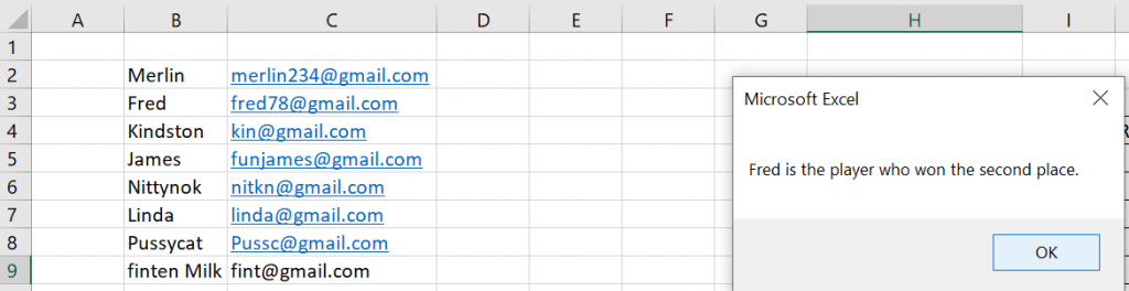
MsgBox runner(1) & " is the player who won the second place. His email id is " & runner(2)

End Sub 

Code explained:

As mentioned in Example 1, we have declared and initialized the variables. Then we use the Index function to find runner (2^nd place) of the match. 

The flow of the program is the same with the difference that here we have been forced to use runner(1) to display value. 

Reason: An Excel range is considered a multidimensional array. Because of this, the return value is not just a string. Instead, it is also an array. To find a value in that array, we have to specify index. 

(1) is used here since there is only one value (or we have specified only 1 column in the range).
To understand it better, if we had used the range Range (“B2:C9” ) in our code, then the return value of the index would have both values in Range (“B2”) and Range(“C2”) i.e. All values of (various columns) of the second row (position parameter given in the Index function).

The image above clearly shows the value of the runner object (the returned value). It has both the name and the email address. Suppose, I want to display the email address of the runner, I will have to display runner(2) in the messagebox.

MsgBox runner(1) & " is the player who won the second place. His email id is " & runner(2)

<!-- /wp:shortcode -->

<!-- wp:image {"id":14452,"sizeSlug":"large","linkDestination":"none"} -->
<figure class="wp-block-image size-large"><img src="https://software-solutions-online.com/wp-content/uploads/2021/06/unnamed-11.png" alt="Excel message box that reads "Fred is the player who won the second place. His email id is [email protected]"" class="wp-image-14452"/></figure>
<!-- /wp:image -->

<!-- wp:heading {"level":3} -->
<h3>Example 3</h3>
<!-- /wp:heading -->

<!-- wp:paragraph -->
<p>In the example below, we get the capital of a state whose index is known. So, we are using an array of two dimensions. If we use formula, we refer to the 4<sup>th</sup> row and 2<sup>nd</sup> column of the selected range. So the value of the cell turns out to be “Patna”.</p>
<!-- /wp:paragraph -->

<!-- wp:image {"id":14457,"sizeSlug":"large","linkDestination":"none"} -->
<figure class="wp-block-image size-large"><img src="https://software-solutions-online.com/wp-content/uploads/2021/06/unnamed-12-1024x266.png" alt="Example of using array to find capital states." class="wp-image-14457"/></figure>
<!-- /wp:image -->

<!-- wp:paragraph -->
<p>Let us do the same using VBA.</p>
<!-- /wp:paragraph -->

<!-- wp:shortcode -->

Sub IndexMatch_demo1()

' declare variables
Dim required_pos, str_capital, arr_states_cap, capital_col

' initialize variables
required_pos = 4
capital_col = 2
arr_states_cap = Range("B2:C16")

'use the function to get the capital
str_capital = Application.WorksheetFunction.Index([arr_states_cap], required_pos, 2)

' display the result
MsgBox str_capital

End Sub

Code explained:

Post declaration and initialization of variables, the Index function is used to get the value  in the 4^th row, 2^nd column of the selected state, capital range of cells on the Excel sheet.

Finally, the output that we see in the message box would be “Patna” which is the capital of Bihar.

The Match Formula and Function 

Here is my article about the Match formula in Excel and Match function in VBA:

Using the Match Function in VBA and Excel – VBA and VB.Net Tutorials, Education and Programming Services (software-solutions-online.com)

Using the Index Function with the Match Function

As we have already understood, the Index function gives the value in the known index of an array. The Match function does the opposite. It provides the index value of an item in an array or range of values.

It is possible to use one of these functions within the other. i.e. Match within Index (or) Index within Match.

Example 1

Here is a table that has details of States, Capitals and another column to describe when it was formed (“Founded on”). We are asked to find the “Founded on” value of the state “Maharashtra”.

Let us assume that we do not know its index. So, initially we will use the Match function to find its index.

Once we get that index, using Index we can get the respective values of that index (rows) against all columns.

Sub IndexMatch_demo()

'declare variables
Dim strstate, arr_states, arr_capitals, arr_founded, rowposition_state, str_capital, str_founded

' initialize variables ( set values for them )
strstate = "Maharashtra"
arr_states = Range("B2:B30")
arr_capitals = Range("C2:C30")
arr_founded = Range("D2:D30")

' find the position of the state in the first array ( 0 here states an exact match)
rowposition_state = Application.WorksheetFunction.Match(strstate, ([arr_states]), 0)

'Find the respective capital and "founded on" values of the said state.
str_capital = Application.WorksheetFunction.Index([arr_capitals], rowposition_state)
str_founded = Application.WorksheetFunction.Index([arr_founded], rowposition_state)

' display all values
Debug.Print str_capital(1)
Debug.Print str_founded(1)

End Sub

Code explained:

The required variables are first declared and then initialized. From these lines, we infer that we are supposed to find the capital and “Founded on” values of  the state “Maharashtra.” So, using the Match function in VBA, we find the position of  the state ”Maharashtra.” Then using the same value as the index, we find the capital and “Founded on” values from the respective arrays and display the same in the Immediate window (using the debug.print statement).

In order to explain this further, three arrays were created in the example. If the ranges quoted for each of these arrays are not within the same range ( row values), then this concept of using the same index (row num here) for finding values in other arrays will not work.  So, let us redo the same with one range as a subset of another range to understand the concept better.

Sub IndexMatch_demo3()

'declare variables
Dim strstate, arr_states, start_pos, end_pos, rowposition_state, str_capital, arr_states_captials

' initialize variables ( set values for them )
strstate = "Maharashtra"
start_pos = 2
end_pos = 30

'dynamic defining of the arrays from the excel sheet. The rows values are not hardcoded here.
arr_states_captials = Range("B" & start_pos & ":D" & end_pos)
arr_states = Range("B" & start_pos & ":B" & end_pos)

' find the position of the state in the states array ( 0 here states an exact match)
rowposition_state = Application.WorksheetFunction.Match(strstate, [arr_states], 0)

'Find the respective capital and "founded on" values of the said state.
str_capital = Application.WorksheetFunction.Index([arr_states_captials], rowposition_state, 2)
str_founded = Application.WorksheetFunction.Index([arr_states_captials], rowposition_state, 3)

' display all values
Debug.Print str_capital
Debug.Print str_founded

End Sub

Code explained:

The difference in this modified code lies in the dynamic building of array range. A single dimensional array is defined in order to find the index using the Match function. Then we find the respective values from the other two columns. The Index function here uses both the row position and col position parameter since the array is multidimensional (a complete picture of this is available in the image above).

Conclusion

In my experience, I see that the Index function can be used with multidimensional arrays but when it comes to the Match function, multidimensional arrays have to be sliced using loops and conditions before being passed as parameters. Using a combination of both these functions (Index and Match), it is possible and easy to point to any value/index/any target in a table or an array or a range of Excel cells. Using them wisely can produce great results.

title	keywords	f1_keywords	ms.prod	api_name	ms.assetid	ms.date	ms.localizationpriority
WorksheetFunction.Index method (Excel)	vbaxl10.chm137090	vbaxl10.chm137090	excel	Excel.WorksheetFunction.Index	4656985a-2864-93ed-31c7-e7a551d68e96	05/23/2019	medium

WorksheetFunction.Index method (Excel)

Returns a value or the reference to a value from within a table or range. There are two forms of the Index function: the array form and the reference form.

Syntax

expression.Index (Arg1, Arg2, Arg3, Arg4)

expression A variable that represents a WorksheetFunction object.

Parameters

Name	Required/Optional	Data type	Description
Arg1	Required	Variant	Array or Reference — a range of cells or an array constant. For references, it is the reference to one or more cell ranges.
Arg2	Required	Double	Row_num — selects the row in array from which to return a value. If row_num is omitted, column_num is required. For references, the number of the row in reference from which to return a reference.
Arg3	Optional	Variant	Column_num — selects the column in array from which to return a value. If column_num is omitted, row_num is required. For reference, the number of the column in reference from which to return a reference.
Arg4	Optional	Variant	Area_num — only used when returning references. Selects a range in reference from which to return the intersection of row_num and column_num. The first area selected or entered is numbered 1, the second is 2, and so on. If area_num is omitted, Index uses area 1.

Return value

Variant

Remarks

Array form

Returns the value of an element in a table or an array, selected by the row and column number indexes.

Use the array form if the first argument to Index is an array constant.

If both the row_num and column_num arguments are used, Index returns the value in the cell at the intersection of row_num and column_num.

If you set row_num or column_num to 0 (zero), Index returns the array of values for the entire column or row, respectively. To use values returned as an array, enter the Index function as an array formula in a horizontal range of cells for a row, and in a vertical range of cells for a column. To enter an array formula, press Ctrl+Shift+Enter.

Row_num and column_num must point to a cell within array; otherwise, Index returns the #REF! error value.

Reference form

Returns the reference of the cell at the intersection of a particular row and column. If the reference is made up of nonadjacent selections, you can pick the selection to look in. If each area in reference contains only one row or column, the row_num or column_num argument, respectively, is optional. For example, for a single row reference, use INDEX(reference,column_num).

After reference and area_num have selected a particular range, row_num and column_num select a particular cell: row_num 1 is the first row in the range, column_num 1 is the first column, and so on. The reference returned by Index is the intersection of row_num and column_num.

If you set row_num or column_num to 0 (zero), Index returns the reference for the entire column or row, respectively.

Row_num, column_num, and area_num must point to a cell within reference; otherwise, Index returns the #REF! error value. If row_num and column_num are omitted, Index returns the area in reference specified by area_num.

The result of the Index function is a reference and is interpreted as such by other formulas. Depending on the formula, the return value of Index may be used as a reference or as a value. For example, the formula CELL("width",INDEX(A1:B2,1,2)) is equivalent to CELL("width",B1). The CELL function uses the return value of Index as a cell reference. On the other hand, a formula such as 2*INDEX(A1:B2,1,2) translates the return value of Index into the number in cell B1.

[!includeSupport and feedback]

Date yes Add (Subtract) Days to a Date Concatenate Dates Convert Date to Number Convert Date to Text Month Name to Number Create Date Range from Dates Day Number of Year Month Name from Date First Day of Month Add (Subtract) Weeks to a Date If Functions with Dates Max Date Number of Days Between Dates Number of Days in a Month Number of Weeks Between Dates Number of Years Between Dates Split Date & Time into Separate Cells Countdown Remaining Days Insert Dates Random Date Generator Using Dynamic Ranges — Year to Date Values Add (Subtract) Years to a Date Date Formula Examples Extract Day from Date Get Day Name from Date Count Days Left in Month / Year Count Workdays Left in Month / Year Get Last Day of Month Last Business Day of Month / Year Number of Work / Business Days in Month Weekday Abbreviations Auto Populate Dates Number of Months Between Dates Quarter from a Date Years of Service Change Date Format Compare Dates Time yes Add (Subtract) Hours to Time Add (Subtract) Minutes to Time Add (Subtract) Seconds to Time Add Up time (Total Time) Time Differences Change Time Format Convert Minutes to Hours Convert Time to Decimal Convert Time to Hours Convert Time to Minutes Convert Time to Seconds Military Time Round Time to Nearest 15 Minutes Overtime Calculator Number of Hours Between Times Convert Seconds to Minutes, Hours, or Time Count Hours Worked Time Differences Time Format — Show Minutes Seconds Text yes Add Commas to Cells Get First Word from Text Capitalize First Letter Clean & Format Phone #s Remove Extra Trailing / Leading Spaces Add Spaces to Cell Assign Number Value to Text Combine Cells with Comma Combine First and Last Names Convert Text String to Date Convert Text to Number Extract Text From Cell Get Last Word Remove Unwated Characters Extract Text Before or After Character How to Split Text String by Space, Comma, & More Remove Special Characters Remove First Characters from Left Substitute Multiple Values Switch First & Last Names w/ Commas Remove Specific Text from a Cell Extract Text Between Characters (Ex. Parenthesis) Add Leading Zeros to a Number Remove Line Breaks from Text Remove all Numbers from Text Reverse Text Remove Non-Numeric Characters Remove Last Character(s) From Right Separate First and Last Names Separate Text & Numbers Round yes Round Formulas Round Price to Nearest Dollar or Cent Round to Nearest 10, 100, or 1000 Round to Nearest 5 or .5 Round Percentages Round to Significant Figures Count yes Count Blank and Non-blank Cells Count Cells Between Two Numbers Count Cells not Equal to Count if Cells are in Range Count Times Word Appears in Cell Count Words in Cell Count Specific Characters in Column Count Total Number of Characters in Column Count Cells that Equal one of two Results Count Cells that do not Contain Count Cells that Contain Specific Text Count Unique Values in Range Countif — Multiple Criteria Count Total Number of Cells in Range Count Cells with Any Text Count Total Cells in a Table Lookup yes Two Dimensional VLOOKUP VLOOKUP Simple Example Vlookup — Multiple Matches Case Sensitive Lookup Case Sensitive VLOOKUP Sum if — VLOOKUP Case Sensitive Lookup Case Sensitive VLOOKUP Find Duplicates w/ VLOOKUP or MATCH INDEX MATCH MATCH Lookup — Return Cell Address (Not Value) Lookup Last Value in Column or Row Reverse VLOOKUP (Right to Left) Risk Score Bucket with VLOOKUP Sum with a VLOOKUP Function VLOOKUP & INDIRECT VLOOKUP Concatenate VLOOKUP Contains (Partial Match) 17 Reasons Why Your XLOOKUP is Not Working Double (Nested) XLOOKUP — Dynamic Columns IFERROR (& IFNA) XLOOKUP Lookup Min / Max Value Nested VLOOKUP Top 11 Alternatives to VLOOKUP (Updated 2022!) VLOOKUP – Dynamic Column Reference VLOOKUP – Fix #N/A Error VLOOKUP – Multiple Sheets at Once VLOOKUP & HLOOKUP Combined VLOOKUP & MATCH Combined VLOOKUP Between Worksheets or Spreadsheets VLOOKUP Duplicate Values VLOOKUP Letter Grades VLOOKUP Return Multiple Columns VLOOKUP Returns 0? Return Blank Instead VLOOKUP w/o #N/A Error XLOOKUP Multiple Sheets at Once XLOOKUP Between Worksheets or Spreadsheets XLOOKUP by Date XLOOKUP Duplicate Values XLOOKUP Multiple Criteria XLOOKUP Return Multiple Columns XLOOKUP Returns 0? Return Blank Instead XLOOKUP Text XLOOKUP with IF XLOOKUP With If Statement Misc. yes Sort Multiple Columns Use Cell Value in Formula Percentage Change Between Numbers Percentage Breakdown Rank Values Add Spaces to Cell CAGR Formula Average Time Decimal Part of Number Integer Part of a Number Compare Items in a List Dealing with NA() Errors Get Worksheet Name Wildcard Characters Hyperlink to Current Folder Compound Interest Formula Percentage Increase Create Random Groups Sort with the Small and Large Functions Non-volatile Function Alternatives Decrease a Number by a Percentage Calculate Percent Variance Profit Margin Calculator Convert Column Number to Letter Get Full Address of Named Range Insert File Name Insert Path Latitute / Longitude Functions Replace Negative Values Reverse List Range Convert State Name to Abbreviation Create Dynamic Hyperlinks Custom Sort List with Formula Data Validation — Custom Formulas Dynamic Sheet Reference (INDIRECT) Reference Cell in Another Sheet or Workbook Get Cell Value by Address Get Worksheet Name Increment Cell Reference List Sheet Names List Skipped Numbers in Sequence Return Address of Max Value in Range Search by Keywords Select Every Other (or Every nth) Row Basics yes Cell Reference Basics — A1, R1C1, 3d, etc. Add Up (Sum) Entire Column or Row Into to Dynamic Array Formulas Conversions yes Convert Time Zones Convert Celsius to Fahrenheit Convert Pounds to Kilograms Convert Time to Unix Time Convert Feet to Meters Convert Centimeters to Inches Convert Kilometers to Miles Convert Inches to Feet Convert Date to Julian Format Convert Column Letter to Number Tests yes Test if a Range Contains any Text Test if any Cell in Range is Number Test if a Cell Contains a Specific Value Test if Cell Contains Any Number Test if Cell Contains Specific Number Test if Cell is Number or Text If yes Percentile If Subtotal If Sumproduct If Large If and Small If Median If Concatentate If Max If Rank If TEXTJOIN If Sum yes Sum if — Begins With / Ends With Sum if — Month or Year to Date Sum if — By Year Sum if — Blank / Non-Blank Sum if — Horizontal Sum Count / Sum If — Cell Color INDIRECT Sum Sum If — Across Multiple Sheets Sum If — By Month Sum If — Cells Not Equal To Sum If — Not Blank Sum if — Between Values Sum If — Week Number Sum Text Sum if — By Category or Group Sum if — Cell Contains Specific Text (Wildcards) Sum if — Date Rnage Sum if — Dates Equal Sum if — Day of Week Sum if — Greater Than Sum if — Less Than Average yes Average Non-Zero Values Average If — Not Blank Average — Ignore 0 Average — Ignore Errors Math yes Multiplication Table Cube Roots nth Roots Square Numbers Square Roots Calculations yes Calculate a Ratio Calculate Age KILLLLLLL Calculate Loan Payments GPA Formula Calculate VAT Tax How to Grade Formulas Find yes Find a Number in a Column / Workbook Find Most Frequent Numbers Find Smallest n Values Find nth Occurance of Character in Text Find and Extract Number from String Find Earliest or Latest Date Based on Criteria Find First Cell with Any Value Find Last Row Find Last Row with Data Find Missing Values Find Largest n Values Most Frequent Number Conditional Formatting yes Conditional Format — Dates & Times Conditional Format — Highlight Blank Cells New Functions XLOOKUP Replaces VLOOKUP, HLOOKUP, and INDEX / MATCH Logical yes AND Checks whether all conditions are met. TRUE/FALSE IF If condition is met, do something, if not, do something else. IFERROR If result is an error then do something else. NOT Changes TRUE to FALSE and FALSE to TRUE. OR Checks whether any conditions are met. TRUE/FALSE XOR Checks whether one and only one condition is met. TRUE/FALSE Lookup & Reference yes FALSE The logical value: FALSE. TRUE The logical value: TRUE. ADDRESS Returns a cell address as text. AREAS Returns the number of areas in a reference. CHOOSE Chooses a value from a list based on it’s position number. COLUMN Returns the column number of a cell reference. COLUMNS Returns the number of columns in an array. HLOOKUP Lookup a value in the first row and return a value. HYPERLINK Creates a clickable link. INDEX Returns a value based on it’s column and row numbers. INDIRECT Creates a cell reference from text. LOOKUP Looks up values either horizontally or vertically. MATCH Searches for a value in a list and returns its position. OFFSET Creates a reference offset from a starting point. ROW Returns the row number of a cell reference. ROWS Returns the number of rows in an array. TRANSPOSE Flips the oriention of a range of cells. VLOOKUP Lookup a value in the first column and return a value. Date & Time yes DATE Returns a date from year, month, and day. DATEDIF Number of days, months or years between two dates. DATEVALUE Converts a date stored as text into a valid date DAY Returns the day as a number (1-31). DAYS Returns the number of days between two dates. DAYS360 Returns days between 2 dates in a 360 day year. EDATE Returns a date, n months away from a start date. EOMONTH Returns the last day of the month, n months away date. HOUR Returns the hour as a number (0-23). MINUTE Returns the minute as a number (0-59). MONTH Returns the month as a number (1-12). NETWORKDAYS Number of working days between 2 dates. NETWORKDAYS.INTL Working days between 2 dates, custom weekends. NOW Returns the current date and time. SECOND Returns the second as a number (0-59) TIME Returns the time from a hour, minute, and second. TIMEVALUE Converts a time stored as text into a valid time. TODAY Returns the current date. WEEKDAY Returns the day of the week as a number (1-7). WEEKNUM Returns the week number in a year (1-52). WORKDAY The date n working days from a date. WORKDAY.INTL The date n working days from a date, custom weekends. YEAR Returns the year. YEARFRAC Returns the fraction of a year between 2 dates. Engineering yes CONVERT Convert number from one unit to another. Financial yes FV Calculates the future value. PV Calculates the present value. NPER Calculates the total number of payment periods. PMT Calculates the payment amount. RATE Calculates the interest Rate. NPV Calculates the net present value. IRR The internal rate of return for a set of periodic CFs. XIRR The internal rate of return for a set of non-periodic CFs. PRICE Calculates the price of a bond. YIELD Calculates the bond yield. INTRATE The interest rate of a fully invested security. Information yes CELL Returns information about a cell. ERROR.TYPE Returns a value representing the cell error. ISBLANK Test if cell is blank. TRUE/FALSE ISERR Test if cell value is an error, ignores #N/A. TRUE/FALSE ISERROR Test if cell value is an error. TRUE/FALSE ISEVEN Test if cell value is even. TRUE/FALSE ISFORMULA Test if cell is a formula. TRUE/FALSE ISLOGICAL Test if cell is logical (TRUE or FALSE). TRUE/FALSE ISNA Test if cell value is #N/A. TRUE/FALSE ISNONTEXT Test if cell is not text (blank cells are not text). TRUE/FALSE ISNUMBER Test if cell is a number. TRUE/FALSE ISODD Test if cell value is odd. TRUE/FALSE ISREF Test if cell value is a reference. TRUE/FALSE ISTEXT Test if cell is text. TRUE/FALSE N Converts a value to a number. NA Returns the error: #N/A. TYPE Returns the type of value in a cell. Math yes ABS Calculates the absolute value of a number. AGGREGATE Define and perform calculations for a database or a list. CEILING Rounds a number up, to the nearest specified multiple. COS Returns the cosine of an angle. DEGREES Converts radians to degrees. DSUM Sums database records that meet certain criteria. EVEN Rounds to the nearest even integer. EXP Calculates the exponential value for a given number. FACT Returns the factorial. FLOOR Rounds a number down, to the nearest specified multiple. GCD Returns the greatest common divisor. INT Rounds a number down to the nearest integer. LCM Returns the least common multiple. LN Returns the natural logarithm of a number. LOG Returns the logarithm of a number to a specified base. LOG10 Returns the base-10 logarithm of a number. MOD Returns the remainder after dividing. MROUND Rounds a number to a specified multiple. ODD Rounds to the nearest odd integer. PI The value of PI. POWER Calculates a number raised to a power. PRODUCT Multiplies an array of numbers. QUOTIENT Returns the integer result of division. RADIANS Converts an angle into radians. RAND Calculates a random number between 0 and 1. RANDBETWEEN Calculates a random number between two numbers. ROUND Rounds a number to a specified number of digits. ROUNDDOWN Rounds a number down (towards zero). ROUNDUP Rounds a number up (away from zero). SIGN Returns the sign of a number. SIN Returns the sine of an angle. SQRT Calculates the square root of a number. SUBTOTAL Returns a summary statistic for a series of data. SUM Adds numbers together. SUMIF Sums numbers that meet a criteria. SUMIFS Sums numbers that meet multiple criteria. SUMPRODUCT Multiplies arrays of numbers and sums the resultant array. TAN Returns the tangent of an angle. TRUNC Truncates a number to a specific number of digits. Stats yes AVERAGE Averages numbers. AVERAGEA Averages numbers. Includes text & FALSE =0, TRUE =1. AVERAGEIF Averages numbers that meet a criteria. AVERAGEIFS Averages numbers that meet multiple criteria. CORREL Calculates the correlation of two series. COUNT Counts cells that contain a number. COUNTA Count cells that are non-blank. COUNTBLANK Counts cells that are blank. COUNTIF Counts cells that meet a criteria. COUNTIFS Counts cells that meet multiple criteria. FORECAST Predict future y-values from linear trend line. FREQUENCY Counts values that fall within specified ranges. GROWTH Calculates Y values based on exponential growth. INTERCEPT Calculates the Y intercept for a best-fit line. LARGE Returns the kth largest value. LINEST Returns statistics about a trendline. MAX Returns the largest number. MEDIAN Returns the median number. MIN Returns the smallest number. MODE Returns the most common number. PERCENTILE Returns the kth percentile. PERCENTILE.INC Returns the kth percentile. Where k is inclusive. PERCENTILE.EXC Returns the kth percentile. Where k is exclusive. QUARTILE Returns the specified quartile value. QUARTILE.INC Returns the specified quartile value. Inclusive. QUARTILE.EXC Returns the specified quartile value. Exclusive. RANK Rank of a number within a series. RANK.AVG Rank of a number within a series. Averages. RANK.EQ Rank of a number within a series. Top Rank. SLOPE Calculates the slope from linear regression. SMALL Returns the kth smallest value. STDEV Calculates the standard deviation. STDEV.P Calculates the SD of an entire population. STDEV.S Calculates the SD of a sample. STDEVP Calculates the SD of an entire population TREND Calculates Y values based on a trendline. Text yes CHAR Returns a character specified by a code. CLEAN Removes all non-printable characters. CODE Returns the numeric code for a character. CONCATENATE Combines text together. DOLLAR Converts a number to text in currency format. EXACT Test if cells are exactly equal. Case-sensitive. TRUE/FALSE FIND Locates position of text within a cell.Case-sensitive. LEFT Truncates text a number of characters from the left. LEN Counts number of characters in text. LOWER Converts text to lower case. MID Extracts text from the middle of a cell. PROPER Converts text to proper case. REPLACE Replaces text based on it’s location. REPT Repeats text a number of times. RIGHT Truncates text a number of characters from the right. SEARCH Locates position of text within a cell.Not Case-sensitive. SUBSTITUTE Finds and replaces text. Case-sensitive. TEXT Converts a value into text with a specific number format. TRIM Removes all extra spaces from text. UPPER Converts text to upper case. VALUE Converts a number stored as text into a number.

Всё о работе с ячейками в Excel-VBA: обращение, перебор, удаление, вставка, скрытие, смена имени.

Содержание:

Table of Contents:

• Что такое ячейка Excel?
• Способы обращения к ячейкам
  • Выбор и активация
  • Получение и изменение значений ячеек
    • Ячейки открытой книги
    • Ячейки закрытой книги 
  • Перебор ячеек
  • Перебор в произвольном диапазоне
• Свойства и методы ячеек
  • Имя ячейки
  • Адрес ячейки
  • Размеры ячейки
• Запуск макроса активацией ячейки

2 нюанса:

1. Я почти везде стараюсь использовать ThisWorkbook (а не, например, ActiveWorkbook) для обращения к текущей книге, в которой написан этот код (считаю это наиболее безопасным для новичков способом обращения к книгам, чтобы случайно не внести изменения в другие книги). Для экспериментов можете вставлять этот код в модули, коды книги, либо листа, и он будет работать только в пределах этой книги. 
2. Я использую английский эксель и у меня по стандарту листы называются Sheet1, Sheet2 и т.д. Если вы работаете в русском экселе, то замените Thisworkbook.Sheets(«Sheet1») на Thisworkbook.Sheets(«Лист1»). Если этого не сделать, то вы получите ошибку в связи с тем, что пытаетесь обратиться к несуществующему объекту. Можно также заменить на Thisworkbook.Sheets(1), но это менее безопасно.

Что такое ячейка Excel?

В большинстве мест пишут: «элемент, образованный пересечением столбца и строки». Это определение полезно для людей, которые не знакомы с понятием «таблица». Для того, чтобы понять чем на самом деле является ячейка Excel, необходимо заглянуть в объектную модель Excel. При этом определения объектов «ряд», «столбец» и «ячейка» будут отличаться в зависимости от того, как мы работаем с файлом.

Объекты в Excel-VBA. Пока мы работаем в Excel без углубления в VBA определение ячейки как «пересечения» строк и столбцов нам вполне хватает, но если мы решаем как-то автоматизировать процесс в VBA, то о нём лучше забыть и просто воспринимать лист как «мешок» ячеек, с каждой из которых VBA позволяет работать как минимум тремя способами:

1. по цифровым координатам (ряд, столбец),
2. по адресам формата А1, B2 и т.д. (сценарий целесообразности данного способа обращения в VBA мне сложно представить)
3. по уникальному имени (во втором и третьем вариантах мы будем иметь дело не совсем с ячейкой, а с объектом VBA range, который может состоять из одной или нескольких ячеек). Функции и методы объектов Cells и Range отличаются. Новичкам я бы порекомендовал работать с ячейками VBA только с помощью Cells и по их цифровым координатам и использовать Range только по необходимости.

Все три способа обращения описаны далее

Как это хранится на диске и как с этим работать вне Excel? С точки зрения хранения и обработки вне Excel и VBA. Сделать это можно, например, сменив расширение файла с .xls(x) на .zip и открыв этот архив.

Пример содержимого файла Excel:

Далее xl -> worksheets и мы видим файл листа

Содержимое файла:

 То же, но более наглядно:

<?xml version="1.0" encoding="UTF-8" standalone="yes"?>
<worksheet xmlns="http://schemas.openxmlformats.org/spreadsheetml/2006/main" xmlns:r="http://schemas.openxmlformats.org/officeDocument/2006/relationships" xmlns:mc="http://schemas.openxmlformats.org/markup-compatibility/2006" mc:Ignorable="x14ac xr xr2 xr3" xmlns:x14ac="http://schemas.microsoft.com/office/spreadsheetml/2009/9/ac" xmlns:xr="http://schemas.microsoft.com/office/spreadsheetml/2014/revision" xmlns:xr2="http://schemas.microsoft.com/office/spreadsheetml/2015/revision2" xmlns:xr3="http://schemas.microsoft.com/office/spreadsheetml/2016/revision3" xr:uid="{00000000-0001-0000-0000-000000000000}">
	<dimension ref="B2:F6"/>
	<sheetViews>
		<sheetView tabSelected="1" workbookViewId="0">
			<selection activeCell="D12" sqref="D12"/>
		</sheetView>
	</sheetViews>
	<sheetFormatPr defaultRowHeight="14.4" x14ac:dyDescent="0.3"/>
	<sheetData>
		<row r="2" spans="2:6" x14ac:dyDescent="0.3">
			<c r="B2" t="s">
				<v>0</v>
			</c>
		</row>
		<row r="3" spans="2:6" x14ac:dyDescent="0.3">
			<c r="C3" t="s">
				<v>1</v>
			</c>
		</row>
		<row r="4" spans="2:6" x14ac:dyDescent="0.3">
			<c r="D4" t="s">
				<v>2</v>
			</c>
		</row>
		<row r="5" spans="2:6" x14ac:dyDescent="0.3">
			<c r="E5" t="s">
				<v>0</v></c>
		</row>
		<row r="6" spans="2:6" x14ac:dyDescent="0.3">
			<c r="F6" t="s"><v>3</v>
		</c></row>
	</sheetData>
	<pageMargins left="0.7" right="0.7" top="0.75" bottom="0.75" header="0.3" footer="0.3"/>
</worksheet>

Как мы видим, в структуре объектной модели нет никаких «пересечений». Строго говоря рабочая книга — это архив структурированных данных в формате XML. При этом в каждую «строку» входит «столбец», и в нём в свою очередь прописан номер значения данного столбца, по которому оно подтягивается из другого XML файла при открытии книги для экономии места за счёт отсутствия повторяющихся значений. Почему это важно. Если мы захотим написать какой-то обработчик таких файлов, который будет напрямую редактировать данные в этих XML, то ориентироваться надо на такую модель и структуру данных. И правильное определение будет примерно таким: ячейка — это объект внутри столбца, который в свою очередь находится внутри строки в файле xml, в котором хранятся данные о содержимом листа.

Способы обращения к ячейкам

Выбор и активация

Почти во всех случаях можно и стоит избегать использования методов Select и Activate. На это есть две причины:

1. Это лишь имитация действий пользователя, которая замедляет выполнение программы. Работать с объектами книги можно напрямую без использования методов Select и Activate.
2. Это усложняет код и может приводить к неожиданным последствиям. Каждый раз перед использованием Select необходимо помнить, какие ещё объекты были выбраны до этого и не забывать при необходимости снимать выбор. Либо, например, в случае использования метода Select в самом начале программы может быть выбрано два листа вместо одного потому что пользователь запустил программу, выбрав другой лист.

Можно выбирать и активировать книги, листы, ячейки, фигуры, диаграммы, срезы, таблицы и т.д.

Отменить выбор  ячеек можно методом Unselect:

Selection.Unselect

Отличие выбора от активации — активировать можно только один объект из раннее выбранных. Выбрать можно несколько объектов.

Если вы записали и редактируете код макроса, то лучше всего заменить Select и Activate на конструкцию With … End With. Например, предположим, что мы записали вот такой макрос:

Sub Macro1()
' Macro1 Macro
    Range("F4:F10,H6:H10").Select 'выбрали два несмежных диапазона зажав ctrl
    Range("H6").Activate          'показывает только то, что я начал выбирать второй диапазон с этой ячейки (она осталась белой). Это действие ни на что не влияет
    With Selection.Interior       
        .Pattern = xlSolid
        .PatternColorIndex = xlAutomatic
        .Color = 65535            'залили желтым цветом, нажав на кнопку заливки на верхней панели
        .TintAndShade = 0
        .PatternTintAndShade = 0
    End With
End Sub

Почему макрос записался таким неэффективным образом? Потому что в каждый момент времени (в каждой строке) программа не знает, что вы будете делать дальше. Поэтому в записи выбор ячеек и действия с ними — это два отдельных действия. Этот код лучше всего оптимизировать (особенно если вы хотите скопировать его внутрь какого-нибудь цикла, который должен будет исполняться много раз и перебирать много объектов). Например, так:

Sub Macro11()
'
' Macro1 Macro
    Range("F4:F10,H6:H10").Select '1. смотрим, что за объект выбран (что идёт до .Select)
    Range("H6").Activate
    With Selection.Interior       '2. понимаем, что у выбранного объекта есть свойство interior, с которым далее идёт работа
        .Pattern = xlSolid
        .PatternColorIndex = xlAutomatic
        .Color = 65535
        .TintAndShade = 0
        .PatternTintAndShade = 0
    End With
End Sub



Sub Optimized_Macro()
    With Range("F4:F10,H6:H10").Interior '3. переносим объект напрямую в конструкцию With вместо Selection
' ////// Здесь я для надёжности прописал бы ещё Thisworkbook.Sheet("ИмяЛиста") перед Range,
' ////// чтобы минимизировать риск любых случайных изменений других листов и книг
' ////// With Thisworkbook.Sheet("ИмяЛиста").Range("F4:F10,H6:H10").Interior
        .Pattern = xlSolid               '4. полностью копируем всё, что было записано рекордером внутрь блока with
        .PatternColorIndex = xlAutomatic
        .Color = 55555                   '5. здесь я поменял цвет на зеленый, чтобы было видно, работает ли код при поочерёдном запуске двух макросов
        .TintAndShade = 0
        .PatternTintAndShade = 0
    End With
End Sub

Пример сценария, когда использование Select и Activate оправдано:

Допустим, мы хотим, чтобы во время исполнения программы мы одновременно изменяли несколько листов одним действием и пользователь видел какой-то определённый лист. Это можно сделать примерно так:

Sub Select_Activate_is_OK()
Thisworkbook.Worksheets(Array("Sheet1", "Sheet3")).Select 'Выбираем несколько листов по именам
Thisworkbook.Worksheets("Sheet3").Activate 'Показываем пользователю третий лист
'Далее все действия с выбранными ячейками через Select будут одновременно вносить изменения в оба выбранных листа

'Допустим, что тут мы решили покрасить те же два диапазона:
Range("F4:F10,H6:H10").Select
    Range("H6").Activate
    With Selection.Interior       
        .Pattern = xlSolid
        .PatternColorIndex = xlAutomatic
        .Color = 65535
        .TintAndShade = 0
        .PatternTintAndShade = 0
    End With

End Sub

Единственной причиной использовать этот код по моему мнению может быть желание зачем-то показать пользователю определённую страницу книги в какой-то момент исполнения программы. С точки зрения обработки объектов, опять же, эти действия лишние.

Получение и изменение значений ячеек

Значение ячеек можно получать/изменять с помощью свойства value. 

'Если нужно прочитать / записать значение ячейки, то используется свойство Value
a = ThisWorkbook.Sheets("Sheet1").Cells (1,1).Value 'записать значение ячейки А1 листа "Sheet1" в переменную "a"
ThisWorkbook.Sheets("Sheet1").Cells (1,1).Value = 1  'задать значение ячейки А1 (первый ряд, первый столбец) листа "Sheet1"

'Если нужно прочитать текст как есть (с форматированием), то можно использовать свойство .text:
ThisWorkbook.Sheets("Sheet1").Cells (1,1).Text = "1" 
a = ThisWorkbook.Sheets("Sheet1").Cells (1,1).Text

'Когда проявится разница:
'Например, если мы считываем дату в формате "31 декабря 2021 г.", хранящуюся как дата
a = ThisWorkbook.Sheets("Sheet1").Cells (1,1).Value 'эапишет как "31.12.2021"
a = ThisWorkbook.Sheets("Sheet1").Cells (1,1).Text  'запишет как "31 декабря 2021 г."

Ячейки открытой книги

К ячейкам можно обращаться:

'В книге, в которой хранится макрос (на каком-то из листов, либо в отдельном модуле или форме)
ThisWorkbook.Sheets("Sheet1").Cells(1,1).Value        'По номерам строки и столбца
ThisWorkbook.Sheets("Sheet1").Cells(1,"A").Value      'По номерам строки и букве столбца
ThisWorkbook.Sheets("Sheet1").Range("A1").Value       'По адресу - вариант 1
ThisWorkbook.Sheets("Sheet1").[A1].Value              'По адресу - вариант 2
ThisWorkbook.Sheets("Sheet1").Range("CellName").Value 'По имени ячейки (для этого ей предварительно нужно его присвоить)

'Те же действия, но с использованием полного названия рабочей книги (книга должна быть открыта)
Workbooks("workbook.xlsm").Sheets("Sheet1").Cells(1,1).Value 'По номерам строки и столбца
Workbooks("workbook.xlsm").Sheets("Sheet1").Cells(1,"A").Value                'По номерам строки и букве столбца
Workbooks("workbook.xlsm").Sheets("Sheet1").Range("A1").Value                 'По адресу - вариант 1
Workbooks("workbook.xlsm").Sheets("Sheet1").[A1].Value                        'По адресу - вариант 2
Workbooks("workbook.xlsm").Sheets("Sheet1").Range("CellName").Value           'По имени ячейки (для этого ей предварительно нужно его присвоить)

Ячейки закрытой книги

Если нужно достать или изменить данные в другой закрытой книге, то необходимо прописать открытие и закрытие книги. Непосредственно работать с закрытой книгой не получится, потому что данные в ней хранятся отдельно от структуры и при открытии Excel каждый раз производит расстановку значений по соответствующим «слотам» в структуре. Подробнее о том, как хранятся данные в xlsx см выше.

Workbooks.Open Filename:="С:closed_workbook.xlsx"    'открыть книгу (она становится активной)
a = ActiveWorkbook.Sheets("Sheet1").Cells(1,1).Value  'достать значение ячейки 1,1
ActiveWorkbook.Close False                            'закрыть книгу (False => без сохранения)

Скачать пример, в котором можно посмотреть, как доставать и как записывать значения в закрытую книгу. 

Код из файла:

Option Explicit
Sub get_value_from_closed_wb() 'достать значение из закрытой книги
Dim a, wb_path, wsh As String
wb_path = ThisWorkbook.Sheets("Sheet1").Cells(2, 3).Value 'get path to workbook from sheet1
wsh = ThisWorkbook.Sheets("Sheet1").Cells(3, 3).Value
Workbooks.Open Filename:=wb_path
a = ActiveWorkbook.Sheets(wsh).Cells(3, 3).Value
ActiveWorkbook.Close False
ThisWorkbook.Sheets("Sheet1").Cells(4, 3).Value = a
End Sub

Sub record_value_to_closed_wb() 'записать значение в закрытую книгу
Dim wb_path, b, wsh As String
wsh = ThisWorkbook.Sheets("Sheet1").Cells(3, 3).Value
wb_path = ThisWorkbook.Sheets("Sheet1").Cells(2, 3).Value 'get path to workbook from sheet1
b = ThisWorkbook.Sheets("Sheet1").Cells(5, 3).Value 'get value to record in the target workbook
Workbooks.Open Filename:=wb_path
ActiveWorkbook.Sheets(wsh).Cells(4, 4).Value = b 'add new value to cell D4 of the target workbook
ActiveWorkbook.Close True
End Sub

Перебор ячеек

Перебор в произвольном диапазоне

Скачать файл со всеми примерами

Пройтись по всем ячейкам в нужном диапазоне можно разными способами. Основные:

1. Цикл For Each. Пример:

   Sub iterate_over_cells()
   
   For Each c In ThisWorkbook.Sheets("Sheet1").Range("B2:D4").Cells
   MsgBox (c)
   Next c
   
   End Sub​

   Этот цикл выведет в виде сообщений значения ячеек в диапазоне B2:D4 по порядку по строкам слева направо и по столбцам — сверху вниз. Данный способ можно использовать для действий, в который вам не важны номера ячеек (закрашивание, изменение форматирования, пересчёт чего-то и т.д.).

2. Ту же задачу можно решить с помощью двух вложенных циклов — внешний будет перебирать ряды, а вложенный — ячейки в рядах. Этот способ я использую чаще всего, потому что он позволяет получить больше контроля над исполнением: на каждой итерации цикла нам доступны координаты ячеек. Для перебора всех ячеек на листе этим методом потребуется найти последнюю заполненную ячейку. Пример кода:

   Sub iterate_over_cells()
   
   Dim cl, rw As Integer
   Dim x As Variant
   
   'перебор области 3x3
   For rw = 1 To 3 ' цикл для перебора рядов 1-3
   
       For cl = 1 To 3 'цикл для перебора столбцов 1-3
           x = ThisWorkbook.Sheets("Sheet1").Cells(rw + 1, cl + 1).Value
           MsgBox (x)
       Next cl
   Next rw
   
   
   
   'перебор всех ячеек на листе. Последняя ячейка определена с помощью UsedRange
   'LastRow = ActiveSheet.UsedRange.Row + ActiveSheet.UsedRange.Rows.Count - 1
   'LastCol = ActiveSheet.UsedRange.Column + ActiveSheet.UsedRange.Columns.Count - 1
   'For rw = 1 To LastRow 'цикл перебора всех рядов
   '    For cl = 1 To LastCol 'цикл для перебора всех столбцов
   '        Действия 
   '    Next cl
   'Next rw
   
   
   End Sub​

3. Если нужно перебрать все ячейки в выделенном диапазоне на активном листе, то код будет выглядеть так:

   Sub iterate_cell_by_cell_over_selection()
       Dim ActSheet As Worksheet
       Dim SelRange As Range
       Dim cell As Range
       
    
       Set ActSheet = ActiveSheet
       Set SelRange = Selection
       
       'if we want to do it in every cell of the selected range
       For Each cell In Selection
       MsgBox (cell.Value)
       
       Next cell
   
   End Sub​

   Данный метод подходит для интерактивных макросов, которые выполняют действия над выбранными пользователем областями.

4. Перебор ячеек в ряду

   Sub iterate_cells_in_row()
       Dim i, RowNum, StartCell As Long
       
       RowNum = 3 'какой ряд
       StartCell = 0 ' номер начальной ячейки (минус 1, т.к. в цикле мы прибавляем i)
       
       For i = 1 To 10 ' 10 ячеек в выбранном ряду
       ThisWorkbook.Sheets("Sheet1").Cells(RowNum, i + StartCell).Value = i '(i + StartCell) добавляет 1 к номеру столбца при каждом повторении
       Next i
   
   End Sub

5. Перебор ячеек в столбце

   Sub iterate_cells_in_column()
       Dim i, ColNum, StartCell As Long
       
       ColNum = 3 'какой столбец
       StartCell = 0 ' номер начальной ячейки (минус 1, т.к. в цикле мы прибавляем i)
       
       For i = 1 To 10 ' 10 ячеек
       ThisWorkbook.Sheets("Sheet1").Cells(i + StartCell, ColNum).Value = i ' (i + StartCell) добавляет 1 к номеру ряда при каждом повторении
       Next i
   
   End Sub​

Свойства и методы ячеек

Имя ячейки

Присвоить новое имя можно так:

Thisworkbook.Sheets(1).Cells(1,1).name = "Новое_Имя"

Для того, чтобы сменить имя ячейки нужно сначала удалить существующее имя, а затем присвоить новое. Удалить имя можно так:

ActiveWorkbook.Names("Старое_Имя").Delete

Пример кода для переименования ячеек:

Sub rename_cell()

old_name = "Cell_Old_Name"
new_name = "Cell_New_Name"

ActiveWorkbook.Names(old_name).Delete
ThisWorkbook.Sheets(1).Cells(2, 1).Name = new_name
End Sub

Sub rename_cell_reverse()

old_name = "Cell_New_Name"
new_name = "Cell_Old_Name"

ActiveWorkbook.Names(old_name).Delete
ThisWorkbook.Sheets(1).Cells(2, 1).Name = new_name
End Sub

Адрес ячейки

Sub get_cell_address() ' вывести адрес ячейки в формате буква столбца, номер ряда
  '$A$1 style
  txt_address = ThisWorkbook.Sheets(1).Cells(3, 2).Address
  MsgBox (txt_address)
End Sub

Sub get_cell_address_R1C1()' получить адрес столбца в формате номер ряда, номер столбца
  'R1C1 style
  txt_address = ThisWorkbook.Sheets(1).Cells(3, 2).Address(ReferenceStyle:=xlR1C1)
  MsgBox (txt_address)
End Sub

  'пример функции, которая принимает 2 аргумента: название именованного диапазона и тип желаемого адреса 
  '(1- тип $A$1 2- R1C1 - номер ряда, столбца)
Function get_cell_address_by_name(str As String, address_type As Integer)
  '$A$1 style
  Select Case address_type
    Case 1
      txt_address = Range(str).Address
    Case 2
      txt_address = Range(str).Address(ReferenceStyle:=xlR1C1)
    Case Else
      txt_address = "Wrong address type selected. 1,2 available"
    End Select
  get_cell_address_by_name = txt_address
End Function

'перед запуском нужно убедиться, что в книге есть диапазон с названием, 
'адрес которого мы хотим получить, иначе будет ошибка
Sub test_function() 'запустите эту программу, чтобы увидеть, как работает функция
  x = get_cell_address_by_name("MyValue", 2)
  MsgBox (x)
End Sub

Размеры ячейки

Ширина и длина ячейки в VBA меняется, например, так:

Sub change_size()
Dim x, y As Integer
Dim w, h As Double

'получить координаты целевой ячейки
x = ThisWorkbook.Sheets("Sheet1").Cells(2, 2).Value
y = ThisWorkbook.Sheets("Sheet1").Cells(3, 2).Value

'получить желаемую ширину и высоту ячейки
w = ThisWorkbook.Sheets("Sheet1").Cells(6, 2).Value
h = ThisWorkbook.Sheets("Sheet1").Cells(7, 2).Value

'сменить высоту и ширину ячейки с координатами x,y
ThisWorkbook.Sheets("Sheet1").Cells(x, y).RowHeight = h
ThisWorkbook.Sheets("Sheet1").Cells(x, y).ColumnWidth = w


End Sub

Прочитать значения ширины и высоты ячеек можно двумя способами (однако результаты будут в разных единицах измерения). Если написать просто Cells(x,y).Width или Cells(x,y).Height, то будет получен результат в pt (привязка к размеру шрифта). 

Sub get_size()
Dim x, y As Integer
'получить координаты ячейки, с которой мы будем работать
x = ThisWorkbook.Sheets("Sheet1").Cells(2, 2).Value
y = ThisWorkbook.Sheets("Sheet1").Cells(3, 2).Value

'получить длину и ширину выбранной ячейки в тех же единицах измерения, в которых мы их задавали
ThisWorkbook.Sheets("Sheet1").Cells(2, 6).Value = ThisWorkbook.Sheets("Sheet1").Cells(x, y).ColumnWidth
ThisWorkbook.Sheets("Sheet1").Cells(3, 6).Value = ThisWorkbook.Sheets("Sheet1").Cells(x, y).RowHeight

'получить длину и ширину с помощью свойств ячейки (только для чтения) в поинтах (pt)
ThisWorkbook.Sheets("Sheet1").Cells(7, 9).Value = ThisWorkbook.Sheets("Sheet1").Cells(x, y).Width
ThisWorkbook.Sheets("Sheet1").Cells(8, 9).Value = ThisWorkbook.Sheets("Sheet1").Cells(x, y).Height

End Sub

Скачать файл с примерами изменения и чтения размера ячеек

Запуск макроса активацией ячейки

Для запуска кода VBA при активации ячейки необходимо вставить в код листа нечто подобное:

3 важных момента, чтобы это работало:

1. Этот код должен быть вставлен в код листа (здесь контролируется диапазон D4)

2-3. Программа, ответственная за запуск кода при выборе ячейки, должна называться Worksheet_SelectionChange и должна принимать значение переменной Target, относящейся к триггеру SelectionChange. Другие доступные триггеры можно посмотреть в правом верхнем углу (2).

Скачать файл с базовым примером (как на картинке)

Скачать файл с расширенным примером (код ниже)

Option Explicit

Private Sub Worksheet_SelectionChange(ByVal Target As Range)

        ' имеем в виду, что триггер SelectionChange будет запускать эту Sub после каждого клика мышью (после каждого клика будет проверяться:
          '1. количество выделенных ячеек и 
          '2. не пересекается ли выбранный диапазон с заданным в этой программе диапазоном.
        ' поэтому в эту программу не стоит без необходимости писать никаких других тяжелых операций

    If Selection.Count = 1 Then 'запускаем программу только если выбрано не более 1 ячейки


    'вариант модификации - брать адрес ячейки из другой ячейки:
    'Dim CellName as String
    'CellName = Activesheet.Cells(1,1).value 'брать текстовое имя контролируемой ячейки из A1 (должно быть в формате Буква столбца + номер строки)
    'If Not Intersect(Range(CellName), Target) Is Nothing Then
    'для работы этой модификации следующую строку надо закомментировать/удалить



        If Not Intersect(Range("D4"), Target) Is Nothing Then 
        'если заданный (D4) и выбранный диапазон пересекаются 
        '(пересечение диапазонов НЕ равно Nothing)

        'можно прописать диапазон из нескольких ячеек:
        'If Not Intersect(Range("D4:E10"), Target) Is Nothing Then
        'можно прописать несколько диапазонов:
        'If Not Intersect(Range("D4:E10"), Target) Is Nothing or Not Intersect(Range("A4:A10"), Target) Is Nothing Then

            Call program 'выполняем программу
        End If
    End If
End Sub

Sub program()

MsgBox ("Program Is running") 'здесь пишем код того, что произойдёт при выборе нужной ячейки


End Sub