
Содержание
- 5 Ways to Increment the Cell Values in Excel
- 1- Use Simple Drag:
- 2- Auto-increment using User-Defined Formula:
- 3- Auto – Increment using CountA Function:
- 4- Use If with the Library functions:
- 5- Increment when New Record Begins:
- Calculate Percentage Change in Excel (% Increase/Decrease Formula)
- Calculate Percentage Change Between Two Values (Easy Formula)
- Percentage Increase
- Percentage Decrease
- Calculate the Value After Percentage Increase/Decrease
- Increase/Decrease an Entire Column with Specific Percentage Value
- Percentage Change in Excel with Zero
- Percentage Change With Negative Numbers
- Both the Values are Negative
- One Value is Positive and One is Negative
- Old Value is Positive and New Value is Negative
- Old Value is Negative and New Value is Positive
5 Ways to Increment the Cell Values in Excel
Microsoft Excel is a powerful tool that is widely used by accountants and finance people to make spreadsheets, reports, sales record, summaries and etc. Regardless of the complexity of task, ‘Serial Number’ is a column which is included in almost all types of worksheets. Sequential serial numbers are usually incremented by 1. None of us like filling this column manually by typing 1, 2, 3 … 1000. How relaxing is the idea of auto-incrementing the serial number values is. Today, we will share some unique ways of adding serial numbers in your excel workbook.
1- Use Simple Drag:
Let us start with the most simple and common way of filling up the column. In the serial number column:
- Type the initial and second value in the first and second cell, respectively.
- Select both the cells and they will be highlighted.
- Move your cursor to the bottom-right of the cells (a plus sign will appear).
- Drag it down till the end of your column.
- All the values will be filled in a sequence automatically.
2- Auto-increment using User-Defined Formula:
You may also be familiar with another simple technique of incrementing serial numbers. We type a user defined formula that takes the previous cell’s address and add 1 to it.
Move the cursor down in the column and press Ctrl + D to copy the formula with appropriate reference cells. You may add any value instead of ‘1’ to generate the next number.
3- Auto – Increment using CountA Function:
We are done with the simple and popular ways of filling up the serial number column. We can also perform the same task using the built-in functions. CountA is a function that counts the number of cells in a range that are not empty. The syntax is very simple. Just type CountA, mention the range of cells and it will calculate the number of items. In our example, we are counting the number of products being entered by the user. B2 will be the starting cell address for the range of Products. The last value varies with the position of your cursor. It is one less than your current cell address. We have typed the following formula in the serial number cell that corresponds with the first product.
‘$’ sign freezes the cell value. i.e., starting address of the range will now remain the ‘B2’. If you remove the ‘$’ sign, the entire trick fails as it would not be able to locate the starting point of range correctly.
You may easily observe the loophole of using CountA. It inserts the serial numbers corresponding to empty cells also. So, we can add a condition that makes sure that serial number is filled only w.r.t some product else it is left blank. We modified the formula as:
4- Use If with the Library functions:
You might have noticed that above mentioned practices fill up the column when you insert the formula for incrementing the values. They do not check whether there is some data associated with the serial number or not. Mostly, we want to assign a serial number as soon as we input any data. We can apply a trick to assign serial numbers using the ‘if’ condition which will insert serial number when data is inputted. This flawless approach will automatically adjust the serial numbers when you delete any item from anywhere in the list.
We will calculate the difference between total number of filled and empty cells in a specified range. Add ‘1’ to this difference to obtain the current serial number. In the serial number column, copy this formula:
=if (B3=””,””, COUNTA ($A$2:A2) +1-COUNTBLANK ($A$2:A2))
B3 is the initial cell address for the Products column.
$A$2 is the cell address of Serial Number column.
CountA is a function that counts the number of cells in a range that are not empty.
CountBlank is a function that counts the number of empty cells in a specified range of cells.
This formula can be taken as a different flavor of the previous formula.
5- Increment when New Record Begins:
While working with records we came across data sets where we need to store different attributes that relate to a single object or item. For example, if you are storing the record of any home product, say telephone, it will have name, model number, color and price. In such cases, serial numbers should be incremented when a new record appears. We can use any one of the attributes to specify the beginning of a new record. The selected attribute will be used in the logical test of ‘If Condition’. In our example, we are using incrementing the serial number when ‘Name’ appears in the ‘Products’ column.
So, this was all for today. We hope that you find these tricks handy and helpful. Stay tuned to master your skills at excel!
Источник
Calculate Percentage Change in Excel (% Increase/Decrease Formula)
When working with data in Excel, calculating the percentage change is a common task.
Whether you working with professional sales data, resource management, project management, or personal data, knowing how to calculate percentage change would help you make better decisions and do better data analysis in Excel.
It’s really easy, thanks to amazing MS Excel features and functions.
In this tutorial, I will show you how to calculate percentage change in Excel (i.e., percentage increase or decrease over the given time period).
So let’s get started!
This Tutorial Covers:
Calculate Percentage Change Between Two Values (Easy Formula)
The most common scenario where you have to calculate percentage change is when you have two values, and you need to find out how much change has happened from one value to the other.
For example, if the price of an item increases from $60 to $80, this could be a scenario where you have to calculate how much increase in percentage happened in this case.
Let’s have a look at examples.
Percentage Increase
Suppose I have the data set as shown below where I have the old price of an item in cell A2 and the new price in cell B2.

The formula to calculate the percentage increase would be:
Below is the formula to calculate the price percentage increase in Excel:
There’s a possibility that you may get the resulting value in decimals (the value would be correct, but need the right format).
To convert this decimal into a percentage value, select the cell that has the value and then click on the percentage icon (%) in the Number group in the Home tab of the Excel ribbon.
In case you want to increase or decrease the number of digits after the decimal, use the Increase/Decrease decimal icons that are next to the percentage icon.
Important: It is important to note that I have kept the calculation to find out the change in new end old price in brackets. This is important because I first want to calculate the difference and then want to divide it by the original price. in case you don’t put these in brackets, the formula will first divide and then subtract (following the order of precedence of operators)
Percentage Decrease
Calculating a percentage decrease works the same way as a percentage increase.
Suppose you have the below two values where the new price is lower than the old price.

In this case, you can use the below formula to calculate the percentage decrease:

Since we are calculating the percentage decrease, we calculate the difference between the old and the new price and then divide that value from the old price.
Calculate the Value After Percentage Increase/Decrease
Suppose you have a data set as shown below, where I have some values in column A and the percentage change values in column B.

Below is the formula you can use to calculate the final value that would be after incorporating the percentage change in column B:
You need to copy and paste this formula for all the cells in Column C.
In the above formula, I first calculate the overall percentage that needs to be multiplied with the value. to do that, I add the percentage value to 1 (within brackets).
And this final value is then multiplied by the values in column A to get the result.
As you can see, it would work for both percentage increase and percentage decrease.
In case you’re using Excel with Microsoft 365 subscription, you can use the below formula (and you don’t need to worry about copy-pasting the formula:
Increase/Decrease an Entire Column with Specific Percentage Value
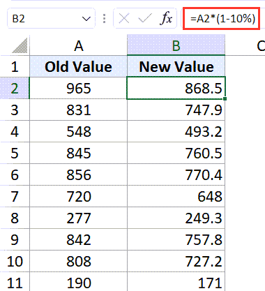
Suppose you have a data set as shown below where I have the old values in column A and I want the new values column to be 10% higher than the old values.

This essentially means that I want to increment all the values in Column A by 10%.
You can use the below formula to do this:
The above formula simply multiplies the old value by 110%, which would end up giving you a value that is 10% higher.
Similarly, if you want to decrease the entire column by 10%, you can use the below formula:
Remember that you need to copy and paste this formula for the entire column.
In case you have the value (by which you want to increase or decrease the entire column) in a cell, you can use the cell reference instead of hardcoding it into the formula.
For example, if I have the percentage value in cell D2, I can use the below formula to get the new value after the percentage change:
The benefit of having the percentage change value in a separate cell is that in case you have to change the calculation by changing this value, you just need to do that in one cell. Since all the formulas are linked to the cell, the formulas would automatically update.
Percentage Change in Excel with Zero
While calculating percentage change in excel is quite easy, you will likely face some challenges when there is a zero involved in the calculation.
For example, if your old value is zero and your new value is 100, what do you think is the percentage increase.
If you use the formulas we have used so far, you will have the below formula:
But you can’t divide a number by zero in math. so if you try and do this, Excel will give you a division error (#DIV/0!)
This is not an Excel problem, rather it’s a math problem.
In such cases, a commonly accepted solution is to consider the percentage change as 100% (as the new value has grown by 100% starting from zero).
Now, what if you had the opposite.
What if you have a value that goes from 100 to 0, and you want to calculate the percentage change.
Thankfully, in this case, you can.
The formula would be:
This will give you 100%, which is the correct answer.
So to put it in simple terms, if you calculating percentage change and there is a 0 involved (be it as the new value or the old value), the change would be 100%
Percentage Change With Negative Numbers
If you have negative numbers involved and you want to calculate the percentage change, things get a bit tricky.
With negative numbers, there could be the following two cases:
- Both the values are negative
- One of the values is negative and the Other one is Positive
Let’s go through this one by one!
Both the Values are Negative
Suppose you have a dataset as shown below where both the values are negative.

I want to find out what’s the change in percentage when values change from -10 to -50
The good news is that if both the values are negative, you can simply go ahead and use the same logic and formula you use with positive numbers.
So below is the formula that will give the right result:

In case both the numbers have the same sign (positive or negative), the math takes care of it.
One Value is Positive and One is Negative
In this scenario, there are two possibilities:
- Old value is positive and new value is negative
- Old value is negative and new value is positive
Let’s look at the first scenario!
Old Value is Positive and New Value is Negative
If the old value is positive, thankfully the math works and you can use the regular percentage formula in Excel.
Suppose you have the dataset as shown below and you want to calculate the percentage change between these values:
The below formula will work:
As you can see, since the new value is negative, this means that there is a decline from the old value, so the result would be a negative percentage change.
So all’s good here!
Now let’s look at the other scenario.
Old Value is Negative and New Value is Positive
This one needs one minor change.
Suppose you’re calculating the change where the old value is -10 and the new value is 10.

If we use the same formulas as before, we will get -200% (which is incorrect as the value change has been positive).
This happens since the denominator in our example is negative. So while the value change is positive, the denominator makes the final result a negative percentage change.
Here is the fix – make the denominator positive.
And here is the new formula you can use in case you have negative values involved:

The ABS function gives the absolute value, so negative values are automatically changes to positive.
So these are some methods that you can use to calculate percentage change in Excel. I have also covered the scenarios where you need to calculate percent change when one of the values could be 0 or negative.
I hope you found this tutorial useful!
Other Excel tutorials you may also like:
Источник
Microsoft Excel is a powerful tool that is widely used by accountants and finance people to make spreadsheets, reports, sales record, summaries and etc. Regardless of the complexity of task, ‘Serial Number’ is a column which is included in almost all types of worksheets. Sequential serial numbers are usually incremented by 1. None of us like filling this column manually by typing 1, 2, 3 … 1000. How relaxing is the idea of auto-incrementing the serial number values is. Today, we will share some unique ways of adding serial numbers in your excel workbook.
1- Use Simple Drag:
Let us start with the most simple and common way of filling up the column. In the serial number column:
- Type the initial and second value in the first and second cell, respectively.
- Select both the cells and they will be highlighted.
- Move your cursor to the bottom-right of the cells (a plus sign will appear).
- Drag it down till the end of your column.
- All the values will be filled in a sequence automatically.
2- Auto-increment using User-Defined Formula:
You may also be familiar with another simple technique of incrementing serial numbers. We type a user defined formula that takes the previous cell’s address and add 1 to it.
A2=A1+1
Move the cursor down in the column and press Ctrl + D to copy the formula with appropriate reference cells. You may add any value instead of ‘1’ to generate the next number.
3- Auto – Increment using CountA Function:
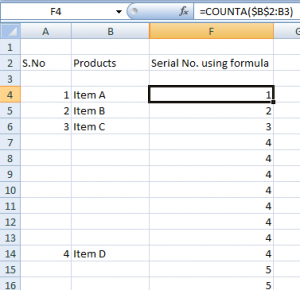
We are done with the simple and popular ways of filling up the serial number column. We can also perform the same task using the built-in functions. CountA is a function that counts the number of cells in a range that are not empty. The syntax is very simple. Just type CountA, mention the range of cells and it will calculate the number of items. In our example, we are counting the number of products being entered by the user. B2 will be the starting cell address for the range of Products. The last value varies with the position of your cursor. It is one less than your current cell address. We have typed the following formula in the serial number cell that corresponds with the first product.
COUNTA($B$2:B3)
‘$’ sign freezes the cell value. i.e., starting address of the range will now remain the ‘B2’. If you remove the ‘$’ sign, the entire trick fails as it would not be able to locate the starting point of range correctly.
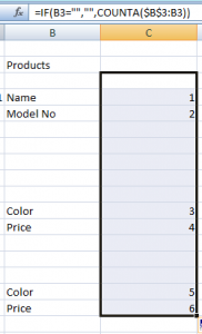
You may easily observe the loophole of using CountA. It inserts the serial numbers corresponding to empty cells also. So, we can add a condition that makes sure that serial number is filled only w.r.t some product else it is left blank. We modified the formula as:
=IF(B3=””,””,COUNTA($B$3:B3))
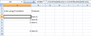
4- Use If with the Library functions:
You might have noticed that above mentioned practices fill up the column when you insert the formula for incrementing the values. They do not check whether there is some data associated with the serial number or not. Mostly, we want to assign a serial number as soon as we input any data. We can apply a trick to assign serial numbers using the ‘if’ condition which will insert serial number when data is inputted. This flawless approach will automatically adjust the serial numbers when you delete any item from anywhere in the list.
We will calculate the difference between total number of filled and empty cells in a specified range. Add ‘1’ to this difference to obtain the current serial number. In the serial number column, copy this formula:
=if (B3=””,””, COUNTA ($A$2:A2) +1-COUNTBLANK ($A$2:A2))
Where,
B3 is the initial cell address for the Products column.
$A$2 is the cell address of Serial Number column.
CountA is a function that counts the number of cells in a range that are not empty.
CountBlank is a function that counts the number of empty cells in a specified range of cells.
This formula can be taken as a different flavor of the previous formula.
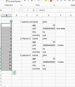
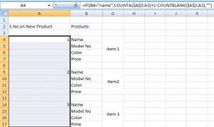
5- Increment when New Record Begins:
While working with records we came across data sets where we need to store different attributes that relate to a single object or item. For example, if you are storing the record of any home product, say telephone, it will have name, model number, color and price. In such cases, serial numbers should be incremented when a new record appears. We can use any one of the attributes to specify the beginning of a new record. The selected attribute will be used in the logical test of ‘If Condition’. In our example, we are using incrementing the serial number when ‘Name’ appears in the ‘Products’ column.
=IF(C4=”name”, COUNTA($B$2:B3)+1-COUNTBLANK($B$2:B3),””)
So, this was all for today. We hope that you find these tricks handy and helpful. Stay tuned to master your skills at excel!
If you want to increment a value or a calculation in Excel with rows and columns as they are copied in other cells, you will need to use the ROW function (not if you have a SEQUENCE function). In this article, we will learn how you can increment any calculations with respect to row or column.
Generic Formula
=Expression + ((ROW()—number of rows above first formula )*[steps])
Expression: This is the value, reference of expression with which you want to increment. It can be a hardcoded value or any expression that returns a valid output. It should be an absolute expression (in most cases).
Number of rows above the first formula: If you are writing this first formula in B3 then the number of rows above this formula will be 2.
[steps]: This is optional. This is the number of steps you want to jump in the next increment.
The Arithmetic operator between expression and formula can be replaced with other operators to suit the requirements of increment.
So that we are familiar with the generic formula, let’s see some examples.
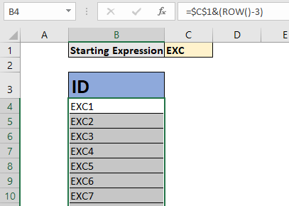
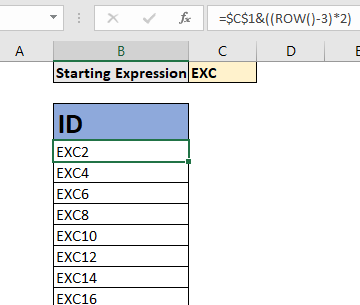
Example 1: Create an Auto Increment Formula for ID Creation.
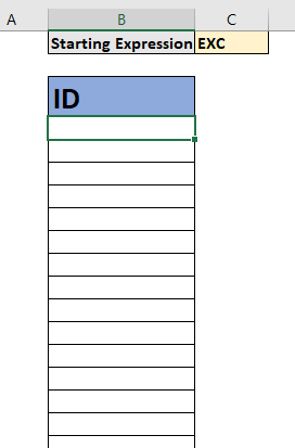
Here, I have to create an auto increment ID formula. I want to write one formula that creates ID as EXC1, EXC2, EXC3 and so on. Since we only need to start the increment by 1 and concatenate it to EXC we don’t use any steps. EXC is written in Cell C1, so we will use C1 as the starting expression.
Using the general formula we write the below formula in Cell B4 and copy it down.
We have replaced the + operator with ampersand operator (&) since we wanted to concatenate. And since we are writing the first formula in Cell B4, we subtract 3 from ROW (). The result is here.
You can see that an auto increment ID has been created. Excel has concatenated 1 to EXC and Added 1 to previous value. You will not need to write any new formula for creating an ID. You just need to copy them down.
Example 2: Increment the ID every 2 steps
If you want to increment the ID every 2 steps then you will need to write this formula.
The result is:
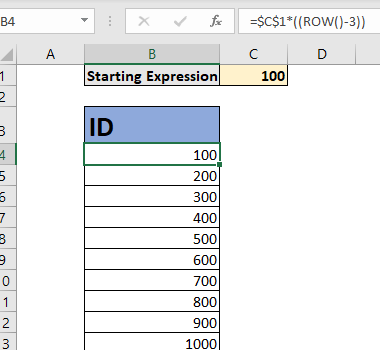
Example 3: Add Original Value with Every Increment
In this increment the starting expression is added to every incremented value. Here’s how it will be if we want to increment the starting value of 100 as 100, 200, 300, and so on.
C1 contains 100.
How does it work?
The technique is simple. As we know, the ROW function returns the current row number it is written in, if now parameter is supplied. The formula above ROW() returns 4.
Next we subtract 3 from it (since there are 3 rows above the 4th row). It gives us 1. This is important. It should be a hard coded value so that it does not change as we copy the formula below.
Finally the value 1 is multiplied (or any other operation) by the starting expression. As we copy the formula below. ROW() returns 5 but subtracting value stays the same (3) and we get 2. And it continues to be the cell you want.
To add steps, we use simple multiplication.
Increment Values By Column
In the above examples we increment by rows. It will not work if you copy them in the next column of the same row.
In the above formula we used the ROW function. Similarly, we can use the COLUMN function.
Generic Formula to Increment by Columns
=Expression + ((COLUMN()—number of columns on left of first formula )*[steps])
Number of columns on the left of the first formula: If you are writing this first formula in B3 then the number of columns on the left of this formula will be 1.
I am not giving any examples as it will be the same as the above examples.
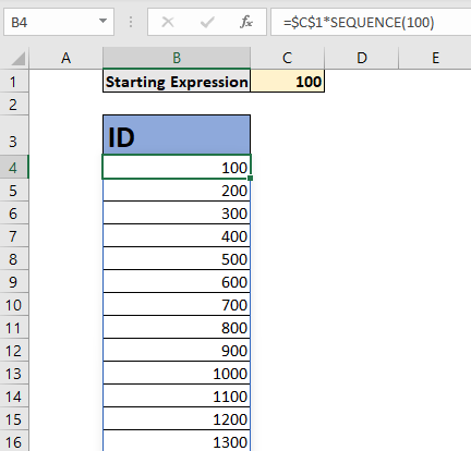
Alternative with SEQUENCE Function
It is a new function only available for EXCEL 365 and 2019 users. It returns an array of sequential numbers. We can use it to increment values sequentially, by rows, columns or both. And yes, you can also include the steps. Using this function you will not need to copy down the formula, as Excel 365 has auto spill functionality.
So, if you want to do the same thing as you did in Example no 3. The SEQUENCE function alternative will be:
It will automatically create 100 increment values in one go without you copying the formula. You can read about the SEQUENCE function here.
So yeah, this is how you can do auto increment in Excel. You can increment the previous cell by adding 1 to it easily now or you add steps to it. I hope this article helped you. If it didn’t solve your problem, let me know the difficulty you are facing, in the comments section below. I will be happy to help you. Till then keep Excelling.
Related Articles:
How To Get Sequential Row Number in Excel | Sometimes we need to get a sequential row number of in table, it can be for a serial number or anything else. In this article, we will learn how to number rows in excel from the start of data.
The SEQUENCE Function in Excel | The SEQUENCE function of Excel returns a sequence of numeric values. You can also adjust the steps in the sequence along with the rows and columns.
Increment a number in a text string in excel | If you have a large list of items and you need to increase the last number of the text of the old text in excel, you will need help of two functions TEXT and RIGHT.
Highlight Row with Bottom 3 Values with a Criteria | If you want to highlight row values with bottom 3 values and with criteria then this formula will help you out.
Popular Articles:
50 Excel Shortcuts to Increase Your Productivity | Get faster at your task. These 50 shortcuts will make you work even faster on Excel.
How to use Excel VLOOKUP Function| This is one of the most used and popular functions of excel that is used to lookup value from different ranges and sheets.
How to use the Excel COUNTIF Function| Count values with conditions using this amazing function. You don’t need to filter your data to count specific values. Countif function is essential to prepare your dashboard.
How to Use SUMIF Function in Excel | This is another dashboard essential function. This helps you sum up values on specific conditions.
When working with data in Excel, calculating the percentage change is a common task.
Whether you working with professional sales data, resource management, project management, or personal data, knowing how to calculate percentage change would help you make better decisions and do better data analysis in Excel.
It’s really easy, thanks to amazing MS Excel features and functions.
In this tutorial, I will show you how to calculate percentage change in Excel (i.e., percentage increase or decrease over the given time period).
So let’s get started!
Calculate Percentage Change Between Two Values (Easy Formula)
The most common scenario where you have to calculate percentage change is when you have two values, and you need to find out how much change has happened from one value to the other.
For example, if the price of an item increases from $60 to $80, this could be a scenario where you have to calculate how much increase in percentage happened in this case.
Let’s have a look at examples.
Percentage Increase
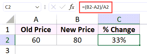
Suppose I have the data set as shown below where I have the old price of an item in cell A2 and the new price in cell B2.
The formula to calculate the percentage increase would be:
=Change in Price/Original Price
Below is the formula to calculate the price percentage increase in Excel:
=(B2-A2)/A2
There’s a possibility that you may get the resulting value in decimals (the value would be correct, but need the right format).
To convert this decimal into a percentage value, select the cell that has the value and then click on the percentage icon (%) in the Number group in the Home tab of the Excel ribbon.
In case you want to increase or decrease the number of digits after the decimal, use the Increase/Decrease decimal icons that are next to the percentage icon.
Important: It is important to note that I have kept the calculation to find out the change in new end old price in brackets. This is important because I first want to calculate the difference and then want to divide it by the original price. in case you don’t put these in brackets, the formula will first divide and then subtract (following the order of precedence of operators)
Percentage Decrease
Calculating a percentage decrease works the same way as a percentage increase.
Suppose you have the below two values where the new price is lower than the old price.
In this case, you can use the below formula to calculate the percentage decrease:
=(B2-A2)/A2
Since we are calculating the percentage decrease, we calculate the difference between the old and the new price and then divide that value from the old price.
Calculate the Value After Percentage Increase/Decrease
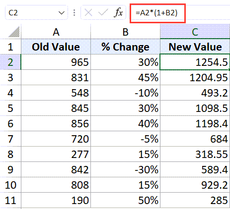
Suppose you have a data set as shown below, where I have some values in column A and the percentage change values in column B.
Below is the formula you can use to calculate the final value that would be after incorporating the percentage change in column B:
=A2*(1+B2)
You need to copy and paste this formula for all the cells in Column C.
In the above formula, I first calculate the overall percentage that needs to be multiplied with the value. to do that, I add the percentage value to 1 (within brackets).
And this final value is then multiplied by the values in column A to get the result.
As you can see, it would work for both percentage increase and percentage decrease.
In case you’re using Excel with Microsoft 365 subscription, you can use the below formula (and you don’t need to worry about copy-pasting the formula:
=A2:A11*(1+B2:B11)
Increase/Decrease an Entire Column with Specific Percentage Value
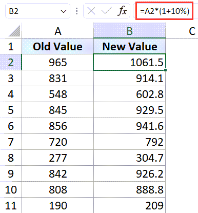
Suppose you have a data set as shown below where I have the old values in column A and I want the new values column to be 10% higher than the old values.
This essentially means that I want to increment all the values in Column A by 10%.
You can use the below formula to do this:
=A2*(1+10%)
The above formula simply multiplies the old value by 110%, which would end up giving you a value that is 10% higher.
Similarly, if you want to decrease the entire column by 10%, you can use the below formula:
=A2*(1-10%)
Remember that you need to copy and paste this formula for the entire column.
In case you have the value (by which you want to increase or decrease the entire column) in a cell, you can use the cell reference instead of hardcoding it into the formula.
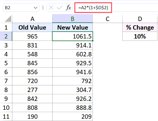
For example, if I have the percentage value in cell D2, I can use the below formula to get the new value after the percentage change:
=A2*(1+$D$2)
The benefit of having the percentage change value in a separate cell is that in case you have to change the calculation by changing this value, you just need to do that in one cell. Since all the formulas are linked to the cell, the formulas would automatically update.
Percentage Change in Excel with Zero
While calculating percentage change in excel is quite easy, you will likely face some challenges when there is a zero involved in the calculation.
For example, if your old value is zero and your new value is 100, what do you think is the percentage increase.
If you use the formulas we have used so far, you will have the below formula:
=(100-0)/0
But you can’t divide a number by zero in math. so if you try and do this, Excel will give you a division error (#DIV/0!)
This is not an Excel problem, rather it’s a math problem.
In such cases, a commonly accepted solution is to consider the percentage change as 100% (as the new value has grown by 100% starting from zero).
Now, what if you had the opposite.
What if you have a value that goes from 100 to 0, and you want to calculate the percentage change.
Thankfully, in this case, you can.
The formula would be:
=(100-0)/100
This will give you 100%, which is the correct answer.
So to put it in simple terms, if you calculating percentage change and there is a 0 involved (be it as the new value or the old value), the change would be 100%
Percentage Change With Negative Numbers
If you have negative numbers involved and you want to calculate the percentage change, things get a bit tricky.
With negative numbers, there could be the following two cases:
- Both the values are negative
- One of the values is negative and the Other one is Positive
Let’s go through this one by one!
Both the Values are Negative
Suppose you have a dataset as shown below where both the values are negative.
I want to find out what’s the change in percentage when values change from -10 to -50
The good news is that if both the values are negative, you can simply go ahead and use the same logic and formula you use with positive numbers.
So below is the formula that will give the right result:
=(A2-B2)/A2
In case both the numbers have the same sign (positive or negative), the math takes care of it.
One Value is Positive and One is Negative
In this scenario, there are two possibilities:
- Old value is positive and new value is negative
- Old value is negative and new value is positive
Let’s look at the first scenario!
Old Value is Positive and New Value is Negative
If the old value is positive, thankfully the math works and you can use the regular percentage formula in Excel.
Suppose you have the dataset as shown below and you want to calculate the percentage change between these values:
The below formula will work:
=(B2-A2)/A2
As you can see, since the new value is negative, this means that there is a decline from the old value, so the result would be a negative percentage change.
So all’s good here!
Now let’s look at the other scenario.
Old Value is Negative and New Value is Positive
This one needs one minor change.
Suppose you’re calculating the change where the old value is -10 and the new value is 10.
If we use the same formulas as before, we will get -200% (which is incorrect as the value change has been positive).
This happens since the denominator in our example is negative. So while the value change is positive, the denominator makes the final result a negative percentage change.
Here is the fix – make the denominator positive.
And here is the new formula you can use in case you have negative values involved:
=(B2-A2)/ABS(A2)
The ABS function gives the absolute value, so negative values are automatically changes to positive.
So these are some methods that you can use to calculate percentage change in Excel. I have also covered the scenarios where you need to calculate percent change when one of the values could be 0 or negative.
I hope you found this tutorial useful!
Other Excel tutorials you may also like:
- How To Subtract In Excel (Subtract Cells, Column, Dates/Time)
- How to Multiply in Excel Using Paste Special
- How to Stop Excel from Rounding Numbers (Decimals/Fractions)
- How to Add Decimal Places in Excel (Automatically)
- How to Convert Serial Numbers to Dates in Excel
- How to Calculate PERCENTILE in Excel
Product IDs, serial numbers and other reference numbers require a unique identifier to avoid confusion when referencing a product or specific data point. Although you can manually enter unique numbers for each item, doing so is tedious and time intensive for long lists. Instead, continuously increment a number in Microsoft Excel to produce these unique identifiers.
Formula Method
-
The most obvious way to increment a number in Excel is to add a value to it. Start with any value in cell A1, and enter «=A1+1» in cell A2 to increment the starting value by one. Copy the formula in A2 down the rest of the column to continuously increment the preceding number. This creates a long list of unique identifiers. You may use any number to increment the value, such as altering the formula to «=A1+567,» to create a less obvious pattern.
Increment Feature
-
Microsoft Excel inherently offers a numbering system to automatically create a series of incremented numbers. Enter any starting value in cell A1. Enter the next value in cell A2 to establish a pattern. Select those two cells and drag the bottom fill handle down the column to create a series of incremental numbers. As an example, entering 12 and 24 in cells A1 and A2 would create the series 12, 24, 36, 48, 60 when copied down to cell A5.
Sorting Incremental Numbers
-
If you need to sort data, opt for Excel’s incremental feature. The formula method works great. However, if you change the order of the cells, the formulas change as well. In contrast, Excel’s increment feature avoids formulas and enters the actual incremented value in the each cell. These numbers do not change, even if you reorder the list.
Paste Values
-
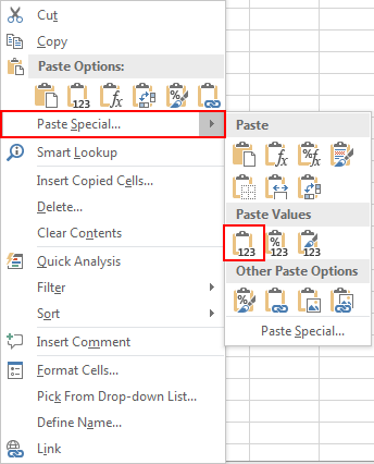
If you don’t want formula-incremented values to change, replace the formulas with the values they create. Select the cells you want to make constant and copy them. Right-click the selected cells and press «V» on your keyboard to replace the formulas with the actual, constant values.
Explanation
In this example, the goal is to increase the prices shown in column C by the percentages shown in column D. For example, given the original price of $70.00, and an increase of 10%, the result should be $77.00. The general formula for this calculation, where «x» is the new price, is:
x=old*(1+percentage)
x=70*(1+10%)
x=70*1.10
x=77.00
Converting this to an Excel formula with cell references, the formula in E5 becomes:
=C5*(1+D5)
=70*(1+0.1)
=70*1.10
=77.00
As the formula is copied down, the formula returns a new price for each item in the table, based on the percentages shown in column D.
Negative percentages
Negative percentages will have the effect of decreasing the original price. For example, with -10% in cell D5 (-0.10), the formula evaluates like this:
=C5*(1+D5)
=70*(1+-0.1)
=70*0.9
=63.00
This example explains the general formula for increasing a number by a given percentage.
Formatting percentages in Excel
In mathematics, a percentage is a number expressed as a fraction of 100. For example, 95% is read as «Ninety-five percent» and is equivalent to 95/100 or 0.95. Accordingly, the values in column D are decimal values, with the Percentage number format applied.
Formula for auto increased serial number in Excel
For auto increase in serial is very easy in excel. It can be done by several ways but in this blog we want it by formula.
Let’s suppose we have 1 in cell A2 and we want to increase serial number in linear method one by one, we can apply =A2+1 in cell A3, copy the formula and paste in below cells up to cell A11. You will get increase number series from 1 to 10.
Another challenge —
Do you face challenges in increasing number basis data in right side adjacent cell and increase the number leaving blank cells? If you know it already, you are welcome to skip it and for the learners let’s learn it with an example.
We have table where before 1st column, we would like to insert formula to increase serial numbers.

Desired result — I want the result according to image «Desired result»

and let’s suppose exists in range G7:G12 and then apply below formula from G9 since G8 contains 1 already as base value.
The formula is —
«=IF(G9=»»,»»,COUNTA(G$8:g9))»
Copy the formula and paste in below cells up to G12.
It will help you in getting desired result.
Thank You!
Best Excel training institute in Noida provides Basic Excel, Advance Excel and VBA offline and online classes.
If you want to learn Excel & VBA courses to be excel expert, connect us on:
ExcelHour
9599408486 / 8929231250
Website: https://www.excelhour.in/
Subscribe to our newsletter
Get the latest posts delivered right to your inbox.
Corporate Trainer at ExcelHour. I have devoted over 9 years to various industries for learning multiple data challenges and trained Excel and VBA courses to the corporate along with offline training.
Great! You’ve successfully subscribed.
Great! Next, complete checkout for full access.
Welcome back! You’ve successfully signed in.
Success! Your account is fully activated, you now have access to all content.
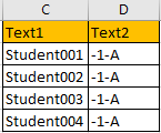
Sometimes we want to fill 1,2,3,4,5… into each cell in a column, for implement this we can enter 1 in the first cell and then drag fill handle down to fill the following cells. But if there are some texts exist with number in cell for example Student001-1-A, we drag down the fill handle, the other cells are only copied the original value, number 001 will not be increased automatically. So, we need to find a simple way that to make number with texts continuous in cells. This article will provide you a simple solution to create increment number with text in cells easily.
Precondition:
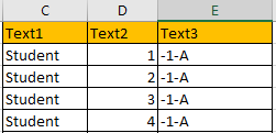
See screenshot below. For student, we use 001,002,003…to identify them, we can type text like ‘Student001-1-A’ one by one manually, but if there are 100 or 1000 students, it will spend a long time to finish this task. So we need simple ways to solve this issue.
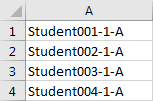
Table of Contents
- Method 1: Create Increment Number with Texts by ‘&’ in Excel
- Method 2: Create Increment Number Within Texts by Formula in Excel
- Related Functions
As we can see the texts are combined as ‘Student00x-1-A’, so we can separate them firstly, then create increment number in one column, and at last combine all texts again. Please see below steps for details.
Step 1: Separate texts in column A to two parts.
(Make sure -1-A is saved in Text format, otherwise error will be displayed)
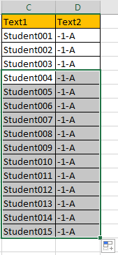
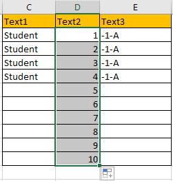
Step 2: Select the range covers column C and column D, drag fill handle down to create increment numbers in column C, and text in column D is copied and pasted.
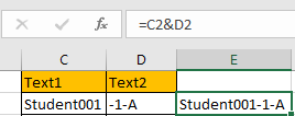
Step 3: In cell E2 enter the formula =C2&D2.
Step 4: Drag down the fill handle in column E till reaching the last data.
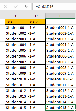
Step 5: Just copy column E, in column A, right click select Paste Special->Paste Values (the first choice).
Then increment numbers within texts are created properly.
Method 2: Create Increment Number Within Texts by Formula in Excel
We can see that in texts ‘Student001-1-A’, except ‘001’ part, other parts are unchanged. So we can extract this part, and then create increment number based on it, and then use formula to combine all parts together.
Step 1: Separate texts ‘Student001-1-A’ to three parts. In column C save ‘Student’, column D save ‘1’, column E save ‘-1-A’.
Step 2: On D2, drag fill handle down to create increment numbers.
Step 3: In F2 enter the formula =$C$2&TEXT(D2,”000″)&$E$2.
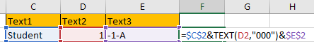
Step 4: Click Enter to check result.
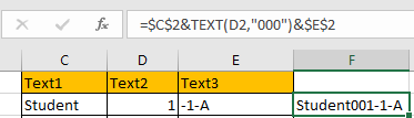
Step 5: Drag the fill handle down to fill cells till the last data.
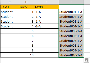
Then you can refer to above method step#5 to copy and paste data properly.
- Excel Text function
The Excel TEXT function converts a numeric value into text string with a specified format. The TEXT function is a build-in function in Microsoft Excel and it is categorized as a Text Function. The syntax of the TEXT function is as below: = TEXT (value, Format code)…
When you view an Excel spreadsheet, you may not even notice an incremented column of numbers running down the left side of the grid. These numbers delineate the rows of the spreadsheet, but you may find that your own work requires incrementing as well, such as when listing different product codes, records or other business finances. While you could simply start at a number and then type every single number after it, you don’t have to. Excel will automatically increment for you; you just have to tell the software what and where.
Step 1
Launch Excel. Type the number to begin the incrementing into the grid, such as “1.”
Step 2
Press the “Enter” key to drop to the cell below and type the next number, such as “2.”
Step 3
Highlight the two cells. Note that when you highlight in Excel, the highlighted cells have a thick black border with a small black box in the bottom-right corner.
Step 4
Hover the cursor over that black box until the cursor turns into a plus symbol. Click and drag that black box straight down, until the border includes the number of increments required. For example, to increment to 30, drag the border until it is aligned with the 30th line of the grid.
Step 5
Click anywhere on the grid to release the border and the increment appears.
References
Resources
Tips
- You need to type at least two numbers for Excel to know you want to increment. Otherwise, if you just type one number and drag the black box, Excel will populate all of the selected cells with that same number.
- You do not have to type two following numbers to increment. Excel can also increment in multiples. For example, if you type a “4” and an “8,” Excel will increment 12, 16, 20, 24 and so on.
Writer Bio
Fionia LeChat is a technical writer whose major skill sets include the MS Office Suite (Word, PowerPoint, Excel, Publisher), Photoshop, Paint, desktop publishing, design and graphics. LeChat has a Master of Science in technical writing, a Master of Arts in public relations and communications and a Bachelor of Arts in writing/English.