In excel workbook you can do this - Word и Excel - помощь в работе с программами

Selecting the header cells, clicking the Home tab, clicking Merge & Center, and then clicking either Merge & Center or Merge Cells will delete any text that is not in the upper-left cell of the selected range.

If you want to split merged cells into their individual cells, you can always unmerge them.

To merge cells

1. Select the cells you want to merge.

2. On the Home tab, in the Alignment group, click the Merge & Center arrow (not the button), and then click Merge Cells.

To merge and center cells

1. Select the cells you want to merge.

2. Click the Merge & Center arrow (not the button), and then click Merge & Center.

To merge cells in multiple rows by using Merge Across

1. Select the cells you want to merge.

2. Click the Merge & Center arrow (not the button), and then click Merge Across.

To split merged cells into individual cells

1. Select the cells you want to unmerge.

2. Click the Merge & Center arrow (not the button), and then click Unmerge Cells.

Customize the Excel 2016 app window

How you use Excel 2016 depends on your personal working style and the type of data collections you manage. The Excel product team interviews customers, observes how differing organizations use the app, and sets up the user interface so that many users won’t need to change it to work effectively. If you do want to change the Excel app window, including the user interface, you can. You can change how Excel displays your worksheets; zoom in on worksheet data; add frequently used commands to the Quick Access Toolbar; hide, display, and reorder ribbon tabs; and create custom tabs to make groups of commands readily accessible.

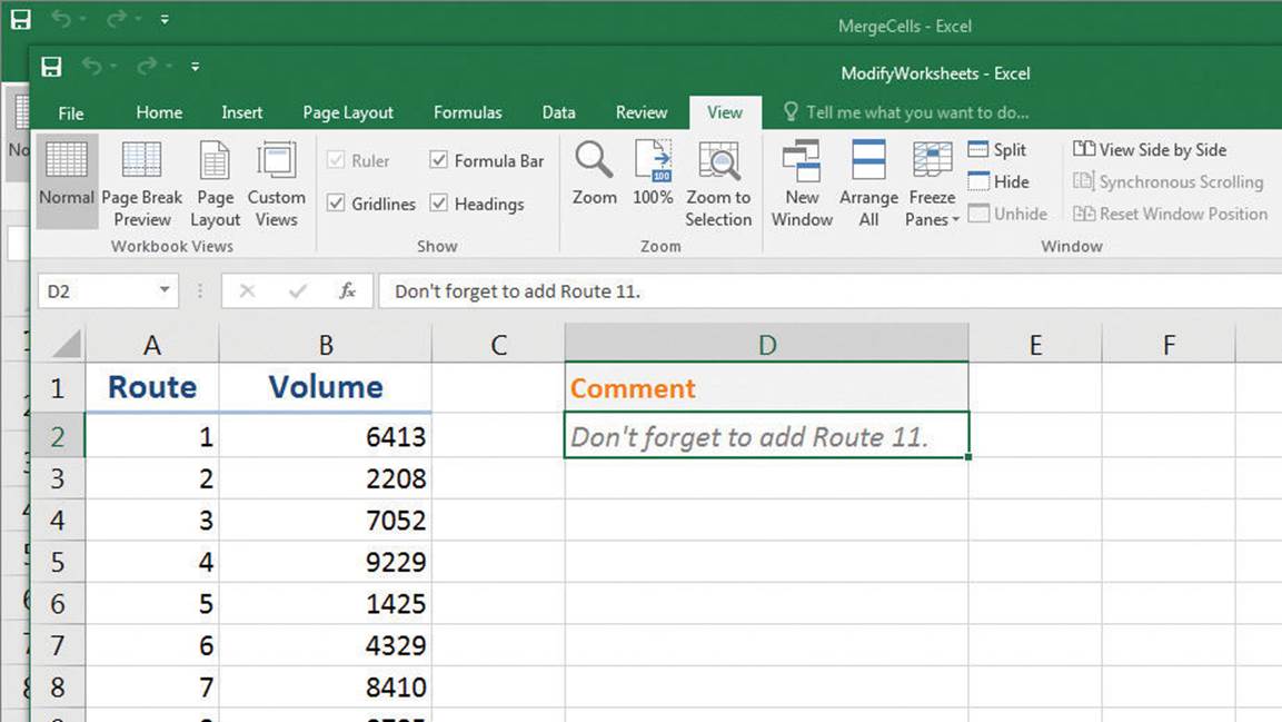
Zoom in on a worksheet

One way to make Excel easier to work with is to change the app’s zoom level. Just as you can “zoom in” with a camera to increase the size of an object in the camera’s viewer, you can use the zoom setting to change the size of objects within the Excel 2016 app window. You can change the zoom level from the ribbon or by using the Zoom control in the lower-right corner of the Excel 2016 window.

Change worksheet magnification by using the Zoom control

The minimum zoom level in Excel 2016 is 10 percent; the maximum is 400 percent.

To zoom in on a worksheet

1. Using the Zoom control in the lower-right corner of the app window, click the Zoom In button (which looks like a plus sign).

To zoom out on a worksheet

1. Using the Zoom control in the lower-right corner of the app window, click the Zoom Out button (which looks like a minus sign).

To set the zoom level to 100 percent

1. On the View tab of the ribbon, in the Zoom group, click the 100% button.

To set a specific zoom level

1. In the Zoom group, click the Zoom button.

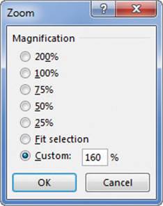
Set a magnification level by using the Zoom dialog box

2. In the Zoom dialog box, enter a value in the Custom box.

3. Click OK.

To zoom in on specific worksheet highlights

1. Select the cells you want to zoom in on.

2. In the Zoom group, click the Zoom to Selection button.

Arrange multiple workbook windows

As you work with Excel, you will probably need to have more than one workbook open at a time. For example, you could open a workbook that contains customer contact information and copy it into another workbook to be used as the source data for a mass mailing you create in Word 2016. When you have multiple workbooks open simultaneously, you can switch between them or arrange your workbooks on the desktop so that most of the active workbook is shown prominently but the others are easily accessible.

Arrange multiple Excel windows to make them easier to access

Many Excel 2016 workbooks contain formulas on one worksheet that derive their value from data on another worksheet, which means you need to change between two worksheets every time you want to see how modifying your data changes the formula’s result. However, an easier way to approach this is to display two copies of the same workbook simultaneously, displaying the worksheet that contains the data in the original window and displaying the worksheet with the formula in the new window. When you change the data in either copy of the workbook, Excel updates the other copy.

If the original workbook’s name is Merge Cells, Excel 2016 displays the name Merge Cells:1 on the original workbook’s title bar and Merge Cells:2 on the second workbook’s title bar.

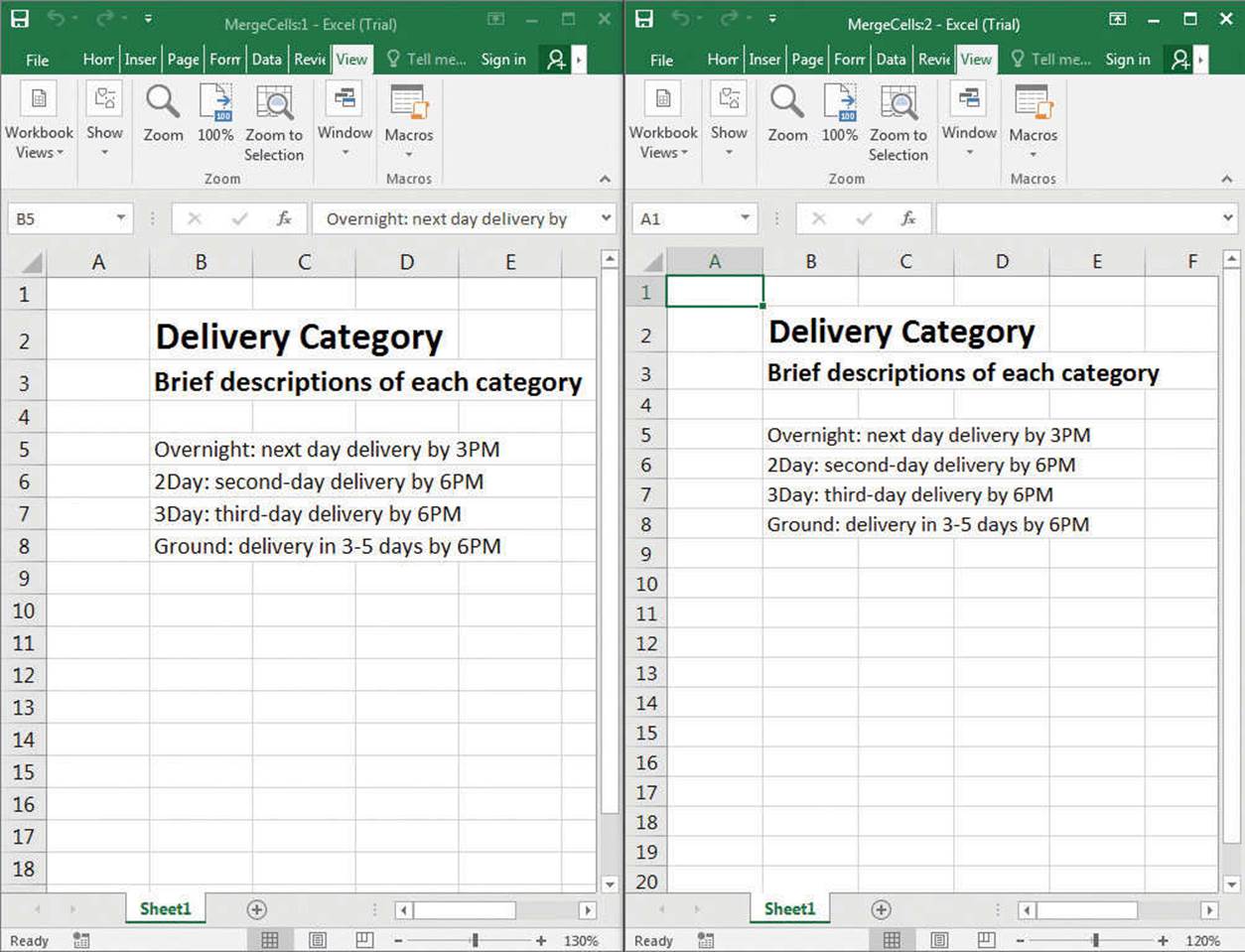
Display two copies of the same workbook side by side

To switch to another open workbook

1. On the View tab, in the Window group, click Switch Windows.

2. In the Switch Windows list, click the workbook you want to display.

To display two copies of the same workbook

1. In the Window group, click New Window.

To change how Excel displays multiple open workbooks

1. In the Window group, click Arrange All.

2. In the Arrange Windows dialog box, click the windows arrangement you want.

3. If necessary, select the Windows of active workbook check box.

4. Click OK.

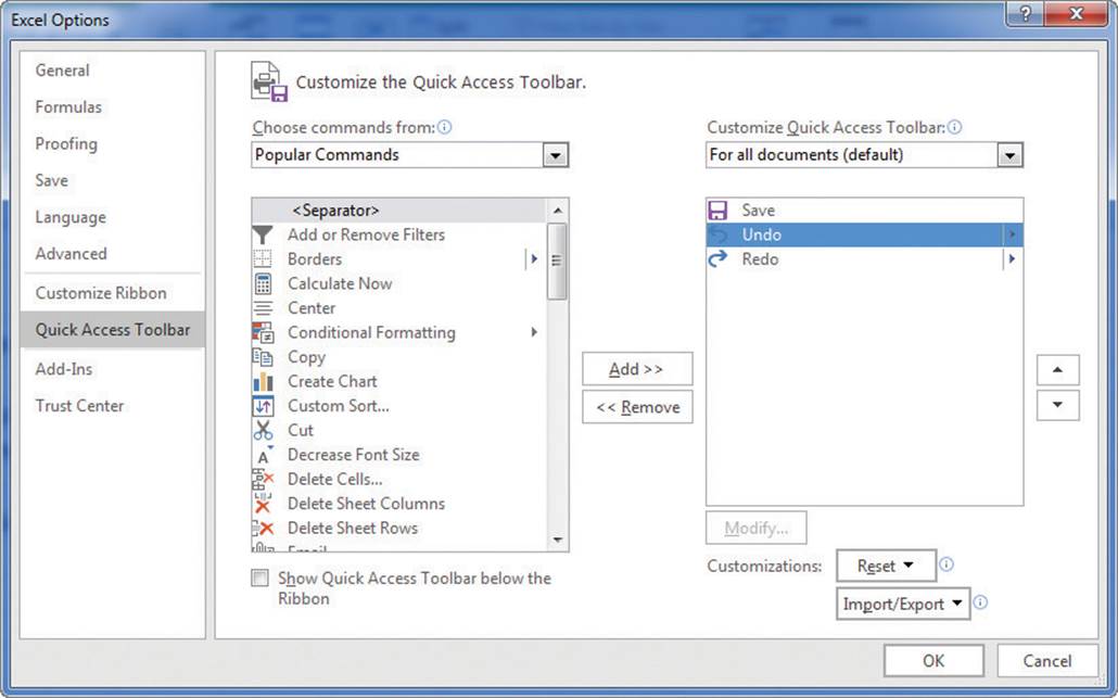
Add buttons to the Quick Access Toolbar

As you continue to work with Excel 2016, you might discover that you use certain commands much more frequently than others. If your workbooks draw data from external sources, for example, you might find yourself using certain ribbon buttons much more often than the app’s designers might have expected. You can make any button accessible with one click by adding the button to the Quick Access Toolbar, located just above the ribbon in the upper-left corner of the Excel app window. You’ll find the tools you need to change the buttons on the Quick Access Toolbar in the Excel Options dialog box.

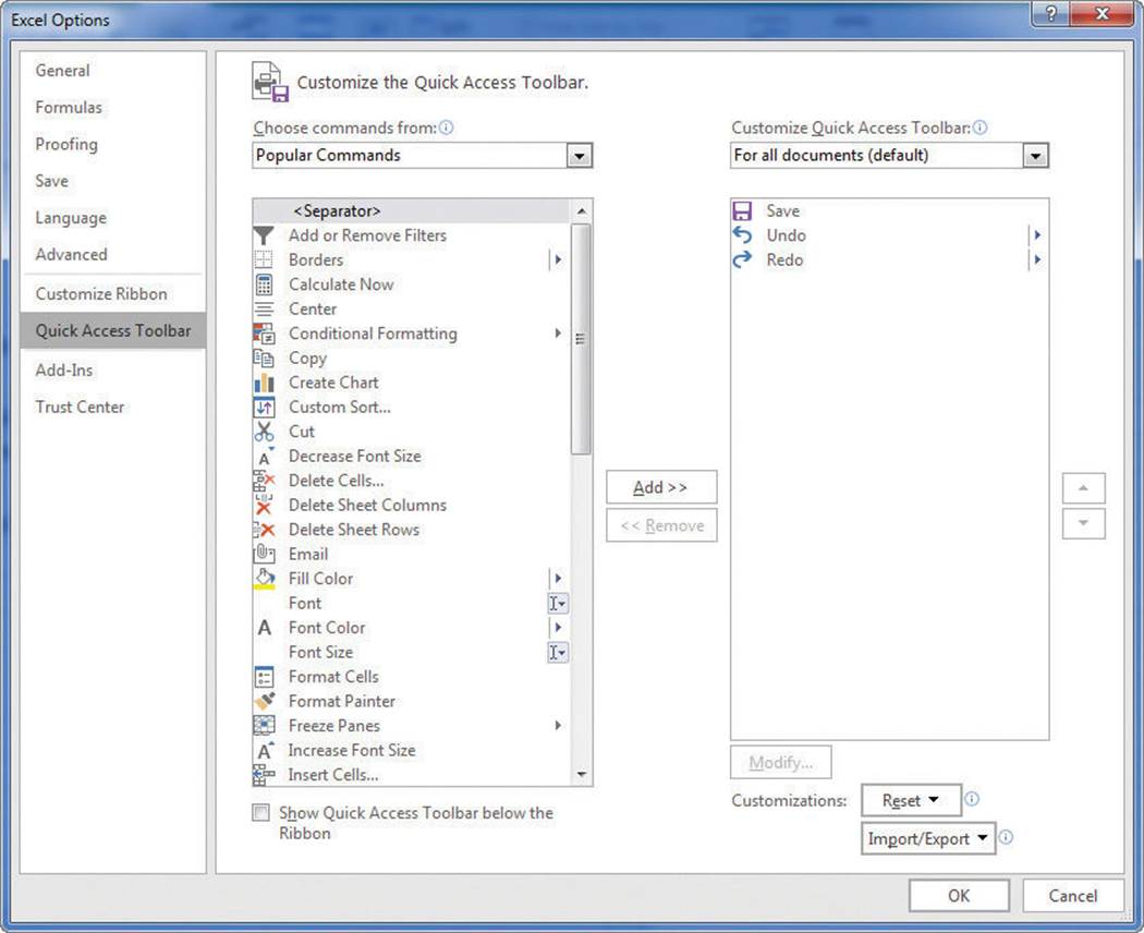
Control which buttons appear on the Quick Access Toolbar

You can add buttons to the Quick Access Toolbar, change their positions, and remove them when you no longer need them. Later, if you want to return the Quick Access Toolbar to its original state, you can reset just the Quick Access Toolbar or the entire ribbon interface.

You can also choose whether your Quick Access Toolbar changes affect all your workbooks or just the active workbook. If you’d like to export your Quick Access Toolbar customizations to a file that can be used to apply those changes to another Excel 2016 installation, you can do so quickly.

To add a button to the Quick Access Toolbar

1. Display the Backstage view, and then click Options.

2. In the Excel Options dialog box, click Quick Access Toolbar.

3. If necessary, click the Customize Quick Access Toolbar arrow and select whether to apply the change to all documents or just the current document.

4. If necessary, click the Choose commands from arrow and click the category of commands from which you want to choose.

5. Click the command to add to the Quick Access Toolbar.

6. Click Add.

7. Click OK.

To change the order of buttons on the Quick Access Toolbar

1. Open the Excel Options dialog box, and then click Quick Access Toolbar.

2. In the right pane, which contains the buttons on the Quick Access Toolbar, click the button you want to move.

Change the order of buttons on the Quick Access Toolbar

3. Click the Move Up button (the upward-pointing triangle on the far right) to move the button higher in the list and to the left on the Quick Access Toolbar.

Click the Move Down button (the downward-pointing triangle on the far right) to move the button lower in the list and to the right on the Quick Access Toolbar.

4. Click OK.

To delete a button from the Quick Access Toolbar

1. Open the Excel Options dialog box, and then click Quick Access Toolbar.

2. In the right pane, click the button you want to delete.

3. Click Remove.

To export your Quick Access Toolbar settings to a file

1. Display the Quick Access Toolbar page of the Excel Options dialog box.

2. Click Import/Export, and then click Export all customizations.

3. In the File Save dialog box, in the File name box, enter a name for the settings file.

4. Click Save.

To reset the Quick Access Toolbar to its original configuration

1. Display the Quick Access Toolbar page of the Excel Options dialog box.

2. Click Reset.

3. Click Reset only Quick Access Toolbar.

4. Click OK.

Customize the ribbon

Excel 2016 enhances your ability to customize the entire ribbon: you can hide and display ribbon tabs, reorder tabs displayed on the ribbon, customize existing tabs (including tool tabs, which appear when specific items are selected), and create custom tabs. You’ll find the tools to customize the ribbon in the Excel Options dialog box.

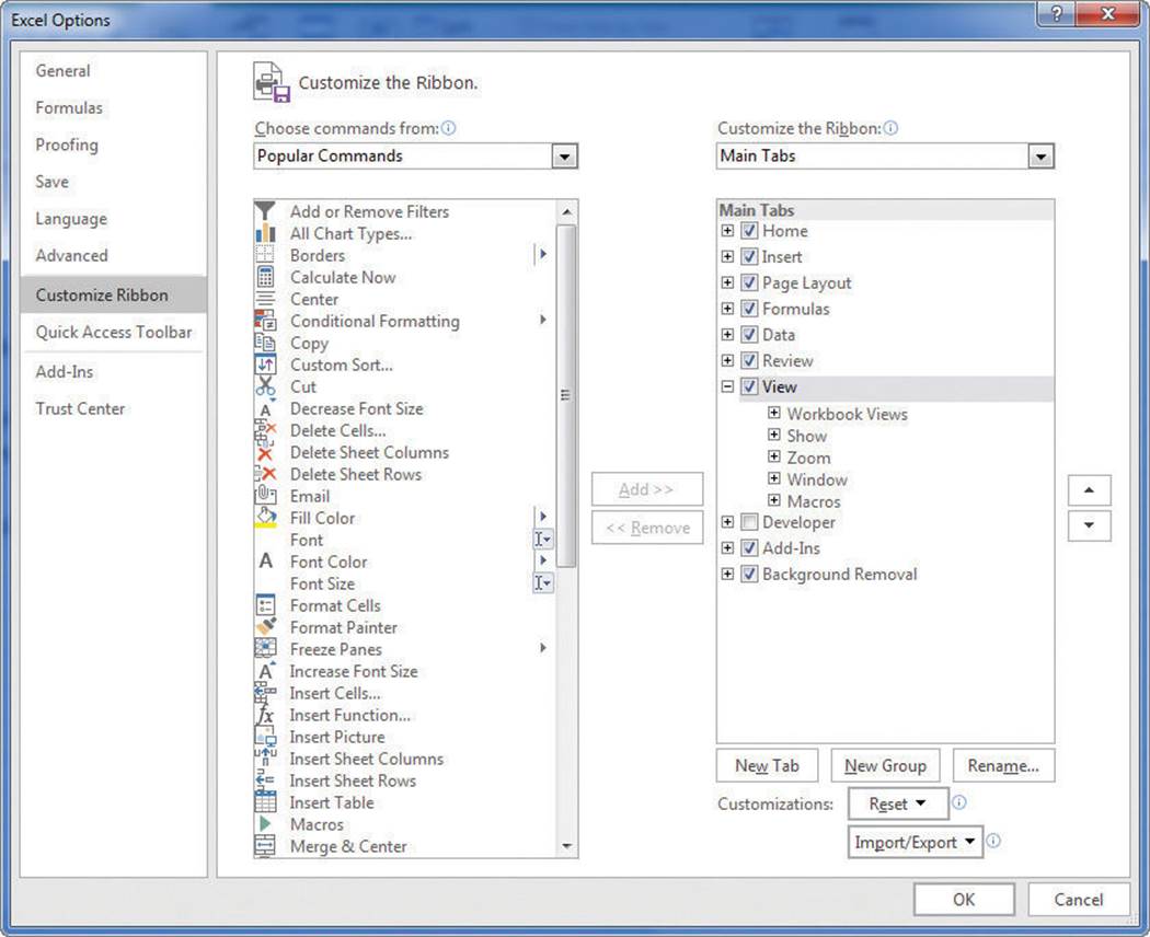
Control which items appear on the ribbon by using the Excel Options dialog box

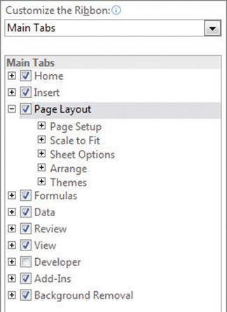
From the Customize Ribbon page of the Excel Options dialog box, you can select which tabs appear on the ribbon and in what order. Each ribbon tab’s name has a check box next to it. If a tab’s check box is selected, that tab appears on the ribbon.

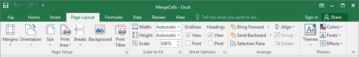
Just as you can change the order of the tabs on the ribbon, with Excel 2016, you can change the order in which groups of commands appear on a tab. For example, the Page Layout tab contains five groups: Themes, Page Setup, Scale To Fit, Sheet Options, and Arrange. If you use the Themes group less frequently than the other groups, you could move the group to the right end of the tab.

Change the order of items on built-in ribbon tabs

You can also remove groups from a ribbon tab. If you remove a group from a built-in tab and later decide you want to restore it, you can put it back without too much worry.

The built-in ribbon tabs are designed efficiently, so adding new command groups might crowd the other items on the tab and make those controls harder to find. Rather than adding controls to an existing ribbon tab, you can create a custom tab and then add groups and commands to it. The default New Tab (Custom) name doesn’t tell you anything about the commands on your new ribbon tab, so you can rename it to reflect its contents.

You can export your ribbon customizations to a file that can be used to apply those changes to another Excel 2016 installation. When you’re ready to apply saved customizations to Excel, import the file and apply it. And, as with the Quick Access Toolbar, you can always reset the ribbon to its original state.

The ribbon is designed to use space efficiently, but you can hide it and other user interface elements such as the formula bar and row and column headings if you want to increase the amount of space available inside the app window.

Tip

Press Ctrl+F1 to hide and unhide the ribbon.

To display a ribbon tab

1. Display the Backstage view, and then click Options.

2. In the Excel Options dialog box, click Customize Ribbon.

3. In the tab list on the right side of the dialog box, select the check box next to the tab’s name.

Select the check box next to the tab you want to appear on the ribbon

4. Click OK.

To hide a ribbon tab

1. In the Excel Options dialog box, click Customize Ribbon.

2. In the tab list on the right side of the dialog box, clear the check box next to the tab’s name.

3. Click OK.

To reorder ribbon elements

1. In the Excel Options dialog box, click Customize Ribbon.

2. In the tab list on the right side of the dialog box, click the element you want to move.

3. Click the Move Up button (the upward-pointing triangle on the far right) to move the button or group higher in the list and to the left on the ribbon tab.

Click the Move Down button (the downward-pointing triangle on the far right) to move the button or group lower in the list and to the right on the ribbon tab.

4. Click OK.

To create a custom ribbon tab

1. On the Customize Ribbon page of the Excel Options dialog box, click New Tab.

To create a custom group on a ribbon tab

1. On the Customize Ribbon page of the Excel Options dialog box, click the ribbon tab where you want to create the custom group.

2. Click New Group.

To add a button to the ribbon

1. On the Customize Ribbon page of the Excel Options dialog box, click the ribbon tab or group to which you want to add a button.

2. If necessary, click the Customize the Ribbon arrow and select Main Tabs or Tool Tabs.

Tip

The tool tabs are the contextual tabs that appear when you work with workbook elements such as shapes, images, or PivotTables.

3. If necessary, click the Choose commands from arrow and click the category of commands from which you want to choose.

4. Click the command to add to the ribbon.

5. Click Add.

6. Click OK.

To rename a ribbon element

1. On the Customize Ribbon page of the Excel Options dialog box, click the ribbon tab or group you want to rename.

2. Click Rename.

3. In the Rename dialog box, enter a new name for the ribbon element.

4. Click OK.

To remove an element from the ribbon

1. On the Customize Ribbon page of the Excel Options dialog box, click the ribbon tab or group you want to remove.

2. Click Remove.

To export your ribbon customizations to a file

1. On the Customize Ribbon page of the Excel Options dialog box, click Import/Export, and then click Export all customizations.

2. In the File Save dialog box, in the File name box, enter a name for the settings file.

3. Click Save.

To import ribbon customizations from a file

1. On the Customize Ribbon page of the Excel Options dialog box, click Import/Export, and then click Import customization file.

Import ribbon settings saved from another Office installation

2. In the File Open dialog box, click the configuration file.

3. Click Open.

To reset the ribbon to its original configuration

1. On the Customize Ribbon page of the Excel Options dialog box, click Reset, and then click Reset all customizations.

2. In the dialog box that appears, click Yes.

To hide or unhide the ribbon

1. Press Ctrl+F1.

To hide or unhide the formula bar

1. On the View tab, in the Show group, select or clear the Formula Bar check box.

To hide or unhide the row and column headings

1. In the Show group, select or clear the Headings check box.

To hide or unhide gridlines

1. In the Show group, select or clear the Gridlines check box.

Skills review

In this chapter, you learned how to:

Explore the editions of Excel 2016

Become familiar with new features in Excel 2016

Create workbooks

Modify workbooks

Modify worksheets

Merge and unmerge cells

Customize the Excel 2016 app window

Practice tasks

The practice files for these tasks are located in the Excel2016SBSCh01 folder. You can save the results of the tasks in the same folder.

Create workbooks

Open the CreateWorkbooks workbook in Excel, and then perform the following tasks:

1. Close the CreateWorkbooks file, and then create a new, blank workbook.

2. Save the new workbook as Exceptions2015.

3. Add the following tags to the file’s properties: exceptions, regional, and percentage.

4. Add a tag to the Category property called performance.

5. Create a custom property called Performance, leave the value of the Type field as Text, and assign the new property the value Exceptions.

6. Save your work.

Modify workbooks

Open the ModifyWorkbooks workbook in Excel, and then perform the following tasks:

1. Create a new worksheet named 2016.

2. Rename the Sheet1 worksheet to 2015 and change its tab color to green.

3. Delete the ScratchPad worksheet.

4. Copy the 2015 worksheet to a new workbook, and then save the new workbook under the name Archive2015.

5. In the ModifyWorkbooks, workbook, hide the 2015 worksheet.

Modify worksheets

Open the ModifyWorksheets workbook in Excel, and then perform the following tasks:

1. On the May 12 worksheet, insert a new column A and a new row 1.

2. After you insert the new row 1, click the Insert Options action button, and then click Clear Formatting.

3. Hide column E.

4. On the May 13 worksheet, delete cell B6, shifting the remaining cells up.

5. Click cell C6, and then insert a cell, shifting the other cells down. Enter the value 4499 in the new cell C6.

6. Select cells E13:F13 and move them to cells B13:C13.

Merge and unmerge cells

Open the MergeCells workbook in Excel, and then perform the following tasks:

1. Merge cells B2:D2.

2. Merge and center cells B3:F3.

3. Merge the cell range B5:E8 by using Merge Across.

4. Unmerge cell B2.

Customize the Excel 2016 app window

Open the CustomizeRibbonTabs workbook in Excel, and then perform the following tasks:

1. Add the Spelling button to the Quick Access Toolbar.

2. Move the Review ribbon tab so it is positioned between the Insert and Page Layout tabs.

3. Create a new ribbon tab named My Commands.

4. Rename the New Group (Custom) group to Formatting.

5. In the list on the left side of the dialog box, display the Main Tabs.

6. From the buttons on the Home tab, add the Styles group to the My Commands ribbon tab you created earlier.

7. Again using the buttons available on the Home tab, add the Number group to the Formatting group on your custom ribbon tab.

8. Save your ribbon changes and click the My Commands tab on the ribbon.

Источник

Who said Excel takes lot of time / steps do something? Here is a list of 15 incredibly fun things you can do to your spreadsheets and each takes no more than 5 seconds to do.

Happy Friday 🙂

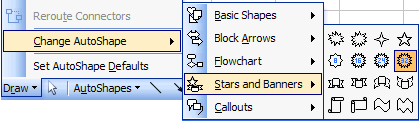
1. Change the shape / color of cell comments

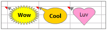
Just select the cell comment, go to draw menu in bottom left corner of the screen, and choose change auto shape option, select a 32 pointed star or heart symbol or a smiley face, just wow everyone 🙂

2. Filter unique items from a list

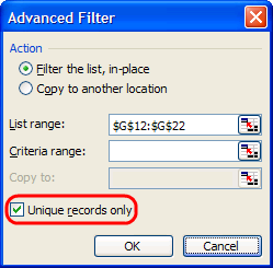
Select the data, go to data > filter > advanced filter and check the “unique items” option.

3. Sort from Left to Right

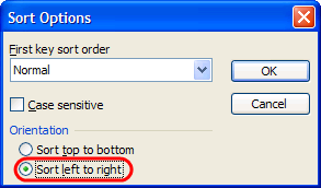
What if your data flows from left to right instead of top to bottom. Just change the sort orientation from “sort options” in the data > sort menu.

4. Hide the grid lines from your sheets

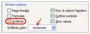
Go to Options dialog in tools menu, uncheck the “grid lines” option to remove gridlines from your worksheets. You can also change the color of grid line from here (not recommended)

5. Add rounded border to your charts, make them look smooth

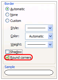
Just right click on the chart, select format chart option, in the dialog, check the “rounded borders”. You can even add a shadow effect from here.

6. Fetch live stock quotes / company research with one click

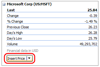
Just enter the stock symbol (MSFT, GOOG, AAPL etc.) in a cell, alt+click on the cell to launch “research pane”, select stock quotes to see MSN Money quotes for the selected symbol. You can fetch company profiles in the same way. Learn more.

7. Repeat rows on top when printing, show table headers on every page

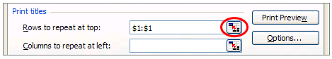
When you are on the sheet view, just hit menu > file > page setup, go to the last tab, specify “rows to repeat”. You can “repeat columns while printing” as well from the same menu.

8. Remove conditional formatting / all formatting with one click

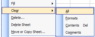
Just go to Menu > Edit > Clear > All to remove all the formatting from selected cell / range.

9. Auto sum cells with one click

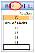
Select a bunch of cells and click on the Sigma symbol on the standard tool bar. Alternatively you can use Alt+= keyboard shortcut.

10. Find width of a column with formula, really!

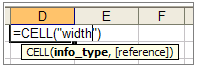
Just use =cell("width") to find the width of the column to which that formula cell belongs. Width is returned as the nearest integer.

11. Find total working days between any two dates, including holidays

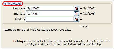
If you work on project plans, gantt charts alot, this can be totally handy. Just type =networkdays(start date, end date, list of holidays) to fetch the number of working days. In the above sample you can see the number of working days between New years day and September first of this year (labor day).

12. Freeze Rows / Columns in your sheet, Show important info even when scrolling

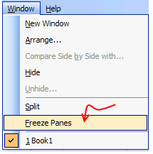
Select the cell diagonally beneath the row / columns you want to freeze (for eg. if you wan to freeze row 1&2 and columns A&B, click in C3), go to menu > window and click on freeze panes.

13. Split sheets in to two, compare side by side to be more productive

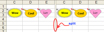
Just click on this little vertical bar on the bottom right corner of the sheet (see below) and drag it to create a vertical split. You can do the same way for a horizontal split as well 🙂

14. Change the color of various sheet name tabs

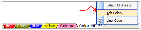
Right click on sheet and select “Tab color” option to change the worksheet tab colors. Group them with similar colors if you have lot of sheets, it looks nice.

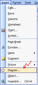
15. Insert a quick organization chart

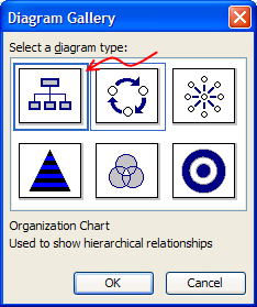
Click on menu > insert > diagram to open the above dialog, just select the organization chart option, enter node values and you have a pretty organization chart. Alternatively learn how to create org charts in excel.

So what do you say now? Isn’t Excel Exciting? 😀

Share this tip with your colleagues

Excel and Power BI tips - Chandoo.org Newsletter

Get FREE Excel + Power BI Tips

Simple, fun and useful emails, once per week.

Learn & be awesome.

121 Comments
Ask a question or say something…
Tagged under

cool, formatting, freeze panes, fun, how to, ideas, Learn Excel, microsoft, Microsoft Excel Formulas, spreadsheet, technology, tips, tricks
Category:

All Time Hits, Featured, hacks, ideas, Learn Excel

Welcome to Chandoo.org

Thank you so much for visiting. My aim is to make you awesome in Excel & Power BI. I do this by sharing videos, tips, examples and downloads on this website. There are more than 1,000 pages with all things Excel, Power BI, Dashboards & VBA here. Go ahead and spend few minutes to be AWESOME.

Read my story • FREE Excel tips book

Excel School made me great at work.

 5/5

Excel formula list - 100+ examples and howto guide for you

From simple to complex, there is a formula for every occasion. Check out the list now.

Calendars, invoices, trackers and much more. All free, fun and fantastic.

Power Query, Data model, DAX, Filters, Slicers, Conditional formats and beautiful charts. It’s all here.

Still on fence about Power BI? In this getting started guide, learn what is Power BI, how to get it and how to create your first report from scratch.

Related Tips

121 Responses to “Excel can be Exciting – 15 fun things you can do with your spreadsheet in less than 5 seconds”

Great tips! Another good one is highlighting a bunch of cells and changing the autosum visual at the bottom right to be Average or Count instead of auto sum.
[…] from a list, sorting data from left to right, freezing panes, and coloring your worksheet tabs. Excel can be Exciting : 15 Fun things to do with Microsoft Excel [Pointy Haired Dilbert — […]
[…] from a list, sorting data from left to right, freezing panes, and coloring your worksheet tabs. Excel can be Exciting : 15 Fun things to do with Microsoft Excel [Pointy Haired Dilbert — […]
Adam says:

one note on the «unique items» tip — this only works with numerical data — if you’re looking to weed out unique text entries, no dice — I work in Excel a lot with names and proprietary tags and would love a way to select a unique text entry — any suggestions?
- badOedipus says:
  
  You can filter duplicate text entries as described above if you use the advanced filter option, however it will not allow you to do an additional filter on an adjacent column afterwards without duplicating the data first.
  The method detailed below will allow you to filter our duplicate entries based on a conditional format.
  
  Select the range from which you wish to filter out duplicate text entries
  Click on Conditional Formatting > New Rule… > Use a formula to determine which cells to format
  type the following formula in the text box: =AND(COUNTIF(«RangeAddress«, «FirstCellAddress«)>1, MATCH(«FirstCellAddress«,»RangeAddress«, 0)<> ROW()) making sure to substitute accordingly. Note: RangeAddress should be absolute(«$A$1:$A$20»), and FirstCellAddress should be relative («A1»).
  Set the format to fill the cells with a color, depending on the application I use either a faint off-white to down play the color or a bright yellow to really make it pop — the choice is yours.
  Ta-da your duplicates are now colored. You can now filter by color if you use 2010 to see only duplicates or only unique records (unique being only one record per value). Pre-2010 you can sort by color to get them at the top/bottom of your list.
- Adrian says:
  
  Maybe if you use Access.
  - Vincent says:
    
    First post on chandoo.org, wahoooo!
    Anyways, after reading the above comments I just realized there’s a similar way to flag duplicate values with a formula, and one that works for strings as well as numbers. If you’re working in column A with a header row then your IDs will be in cells A2:A___. The following formula can be entered in B2 and filled downward to return FALSE when the ID is a repeated value, i.e. it is not the first instance of that value:
    «=MATCH(A2,$A$2:$A$__,0)=(ROW(A2)-ROW($A$1))».
    - Martin says:
      
      Re: =MATCH(A2,$A$2:$A$__,0)=(ROW(A2)-ROW($A$1))
      
      That’s a brilliant formula — I shall use that.
      
      Many thanks for sharing!
- Jason C says:
  
  Just highlight duplicates and then filter out the highlighted cells.
Mazy says:

OK, my hint, I think this excel function have never been documented or referred even in manuals:)

If you want to insert a part of a worksheet as picture (e.g. you want to include a small chart to a preformatted excel document), do the following:

DRAW anything, a square, circle, etc.
SELECT the cells you want to insert as a picture
SELECT the object you made (square,etc.)
PASTE

Voila:)
PK says:

I can’t get the comment to change. It just wants to draw a new autoshape.
- Tom says:
  
  To change the shape of the comment In Excel 2010 — I had to Customize the Ribbon [FILE, OPTIONS] and add a «Format» tab to the Main Tabs to allow the Format tab to be available all the time. Now I can Edit the shape.
@Adam.. It works for text data for me, which version of excel you are using, all these tips are tested in Excel 2003.

@PK … when you select comment to edit (shift+f2) click on the border of the comment, then go to bottom left corner in the screen and select draw > change auto shape. Should work in excel 2003 and above. Let me know if you see some problems 🙂
- Renate Callahan says:
  
  nope, it still doesn’t work. There is no draw -> change auto shape available for me. The left bottom corner of the screen just shows ‘Ready’ and if I right click on it it shows a lot of other things to activate, none of it is Draw or Auto options. I use Excel 2007
MM says:

You’ve missed an important step in your first tip. The Drawing toolbar must be active for this to work. Mine is not on by default, so I have to take the extra set to turn it on.
Jason says:

Very nice, thanks!

Could you clarify «You can also change the color of grid line from here (not recommended)» What is the recommended method.
The graphic designer-side of my job hates Excel, but the business owner side of me finds it to be essential. These tips help bring both sides (designer / business owner) closer together. Thanks!
@MM.. you are right, I have assumed the draw toolbar is on… thanks for pointing it out.

@Jason… “You can also change the color of grid line from here (not recommended)”, I said that to convey changing grid line colors is not recommended, as it can scare people or otherwise make your sheet look extremely busy… but you can change the color if you wish.. 😀
I use the NETWORKDAYS function all the time and it just blows people away.
Dude,
networkdays is my fav.

🙂
Nice post.

-Nikhil
My favorite excel command Ctrl and ~
displays all formulas
Thanks you pointy haired Dilbert, this is definitely a great list, like always bookmarked for future uses 😀
greats tips
i like command for displaying all formulas
thanks
Wade says:

Great tips!
However, #14 You need to right-click on the tab not the sheet.
#10 You can just left click and hold on the right most line of the column letter. Also, another tip a lot of users don’t know is that you can change a section of columns you want to one width by highlighting a column with the width you prefer and left-click-hold on the bottom right corner of that column letter and drag it through as many columns as you need.
Excel can be Exciting : 15 Fun things to do with Microsoft Excel | Pointy Haired Dilbert — Chandoo.o…

Who said Excel takes lot of time steps do something Here is a list of 15 incredibly fun things you can do to your spreadsheets and each takes no more than 5…
hey says:

Great history class. Should have gone for Excel 97 while you were at it 😉
0751firewire says:

Hey, HEY

Don’t be rude. It’s a waste of everyone’s time — including yours. Totally unnecessary.

******
Thanks for this post! I really enjoyed reading these tips. I will bookmark this post and will also subscribe to your weekly newsletter!

Thanks so much.
@Wade: you are right, you have to click on sheet name and not on sheet

and #10 was meant to show another way to find column width, but yeah, I always use the left click hold technique to see if the width is enough for me. Thanks for sharing it with everyone 🙂

@0751firewire: thanks 🙂

@everyone… I am happy so many of you liked this post and enjoyed these small but very useful stuff hidden away in the Excel.
- LEO DA VINCI says:
  
  Dear Chandoo,
  I have discovered you only 3 days back . I want a help from you . I am using a software which makes a grid file of lat,long and elevn. data (x,y,z) on 25m into 25m mesh size . I feel that this grid file which is made from a xcel csv sheet containing random x,y,z points can be made on xcel sheet itself. Can i do that ? example of a source data shown below
  
  x y z
  100 50 12.5
  200 40 14.0
  220 75 12.0
  202 60 15.0
  - @Leo Da Vinci
    You can either import and existing CSV file or setup the file directly in Excel as a workbook
  - whatever says:
    
    You can not make a grid gragh on xeel because it has boxes you would have too get speacial advanced software like the sciencestes do:
    
    i know more that somebody from the GEEK squad!!
    - @Whatever
      Can you post a sample of a Grid Graph or a link where we can see what your referring to?
[…] Excel can be Exciting : 15 Fun things to do with Microsoft Excel | Pointy Haired Dilbert — Chandoo.o… […]
Tip #13: In case anyone is an excel newbie like me, to remove the new vertical bar, just double click on the bar.
- Rufus says:
  
  Thanks fir the tip re vertical bar.
  I am a baby Excel beginner at 86!!!!!
Roger says:

Unique text entries can be found easily — use COUNTIF function for each row. You can use autofilter to delete anything with result > 1.
LD says:

To the person joking about Excel 97 — that version of Office is still the standard at my workplace. No joke.
[…] Excel can be Exciting : 15 Fun things to do with Microsoft Excel | Pointy Haired Dilbert — Chandoo.o… […]
shivshankar says:

Adv
[…] Find total working days between any two dates, including holidays […]
Arti says:

I tried second tip to remove the duplicate entries from the row by copying it in another location but its not working if I use data in A’ th column as

A1 aa
A2 aa
A3 bb

and I am trying to copy the unique records to column B.
The above scenario is not working if duplicate entries are present in A1 and A2.
It will work if duplicate entries are present below first record.
Robert says:

@Arti

Autofilter as well as advanced filter needs titles of the columns in the first row. If you have only the three items in your list, Excel assumes, the first «aa» is the title (field name) of your list, not an entry in the list itself. As a result, Excel writes into column B again the first aa as the title and the second aa and bb as the 2 entires.

Simply insert a row above your list and give your list a name in cell A1. Then it should work.
[…] more than 5 seconds to do. Happy Friday 1. Change the shape / color of cell comments Just select thhttp://chandoo.org/wp/2008/08/01/15-fun-things-with-excel/MI-INFO Tutorials — Excel BasicsFor large worksheets that span more than one screen of […]
[…] Excel can be Exciting : 15 Fun things to do with Microsoft Excel […]
[…] on September 13, 2008 Few weeks back, I came across a post about some useful tips in MS Excel — Excel can be exciting . So, I thought I’ll collate some of the helpful tips and tricks that I’ve come across while […]
[…] 15 Fun things you can do with Excel […]
Melli says:

Nr. 5
-> does not work. And I have Excel 2003!
@Melli .. Welcome to PHD…

Are you sure rounded borders are not working. I have made this example in Excel 2003 and they are working alright for me. You have to select the entire chart to change borders to rounded, not the plot area alone.
[…] Excel can be Exciting : 15 Fun things to do with Microsoft Excel | Pointy Haired Dilbert — Chandoo.o… (tags: work windows useful tutorials tutorial tricks toread tools) […]
[…] But often we leave the last steps for manual processing. The article addresses one such problem (extracting unique cells from a range) and tells us how we can automate the whole […]
homepage templates…

I just wanted to share this nice address, where you can get wordpress themes for free. I use one of the designs for my own blog and it was really easy to install. Just activating it in admin and the job was done. :-)…
I did not know excel is this much fun.
Ketan says:

@ Adam & Chandoo…
For removing / filtering the duplicate entry / unique data…one can use the readymade menu from JMT utilities….very useful…
[…] Using Advanced Data Filter […]
[…] Excel can be Exciting — 15 fun things you can do with excel […]
rayna says:

Thx so much PHD…tusi gr8 ho ji…:)
[…] > and un-check grid lines option. (Excel 2007: office button > excel option > advanced)… Get Full Tip 50. To hide a worksheet, go to menu > format > sheet > hide… Get Full Tip 51. To align […]
[…] Beautiful City Photography» and «10 Companies Hiring for Work from Home». (They’ve also included «15 fun things to do with Microsoft Excel», which may be the most terrifying title in blogging […]
[…] Learn Excel Formulas in Plain English | Executive Dashboards in Excel — 4 Part Tutorial | 15 Excel Fun Tips […]
[…] Related: How to change the shape of cell comments from rectangle to any other shape […]
[…] Learn how to color excel worksheet tabs. […]
[…] on excel comments: change the shape of excel comment box | pimp your comment boxes | extract comments using […]
Francis says:

i cannot find CHANGE AUTO SHAPE option in Excel 2007 to design my comment box. Please help?
- @Francis… Excel 2007 has made it little difficult to change comment shapes, but it is still possible. First add a regular shape (like rectangle) to the worksheet. Now select it. This will show a new ribbon called «format». From here, you can find the change shape tool. Add this tool to Quick Access Bar.
  
  Now Select the comment cell and edit comment. At this point, use the change shape tool from QAT to change the shape of comment.
  - Renate Callahan says:
    
    all right!! Thanks, this answers my question posted above. Yes, now it does work and it looks great! 🙂
Ken Buffong says:

Its really made easy.
Paul says:

Its a bit of a faff in 2007, not sure if its just my work computer than won’t let me change the default shape for comment boxes… But for this one workbook i’ve added a simple:

ActiveCell.Comment.Shape.Select
Selection.ShapeRange.AutoShapeType = msoShapeVerticalScroll

Or you can change msoShapeVeriticalScroll to any shape you like…
VENKATRAMAN V S says:

Dear All

Thank you all very much. You guys have taught me a lot of new things in Excel. Keep continuing the good work.
nazia says:

thanx so much…it really is of gr8 gr8 help to me…… :))
The color sheet tab option has disappeared. Was there and working fine but now when I right click there isn’t an option to change the color of my sheets. How can I get this option back?
- @Deanna.. you can reach this from Format button on home ribbon. Key board short code — ALT + HOT (just press h,o and t one after another).
Sanjay says:

Hello,

Can I know the name of the last person who saved the file last.

In a team of 10 members working on a shared excel file, this information will help me to know the name of the person who modified the file.
Shouvik says:

@Sanjay: Open the workbook — Click on File -> Properties -> Click on the Statistics Tab for the information you are looking for.
mer says:

Wish I could see those images, because they’re now blocked by photobucket. Next time use imgur, or host it on your own server.
mimi says:

Brilliant!
Helped me teach my pupils loads in I.C.T today!
LOL
irha says:

you don’t have references 🙁
Hussein says:

I liked a lot this web site

thanks
Rahul aggarwal says:

@chandoo ji
can we change default comment cell box shape in excel 2007or 2010?
saravanan says:

Hi Friends

Can we Increase the Column width >500 in excel 2003.

Pls help…
losraiders says:

I really like tip #1 but I’m how can you do it if you’re using Excel 2007. I don’t see the drawing toolbar…I believe it’s gone in 2007 but not certain. I did see the autoshape when I select the commnent and right click but nothing happens when I select it.
- This is possible in Excel 2007 (and 2010) too. Follow below steps:
  1. Add any drawing shape.
  2. Select it and go to format ribbon
  3. Right click on Edit shape and add it to «Quick Access toolbar»
  4. Now, remove the shape
  5. Select comment cell.
  6. Edit comment.
  7. Use quick access toolbar to change the shape to anything you want.
  - Sudhir says:
    
    This is awesome Chandoo ! Tip#1 I was most impressed. #6 I was not able to replicate — if you meant Alt + (Mouse left) click, it did not work. But manually triggered the reference — but was unable again to make it available as embedded «auto look up» in the sheet itself.
steve says:

wow! this site is awesome
Some tricks are not working with Excel 2003

But others are too cool thanx
[…] and un-check grid lines option. (Excel 2007: office button > excel option > advanced)… Get Full Tip 50. To hide a worksheet, go to menu > format > sheet > hide… Get Full Tip 51. To […]
[…] Using too many tab colors on your excel workbooks [how to do this] […]
Can anyone help. I want to be able to hide a row for exampe row A if the Cell A1 is empty after i have sorted the rows.
I can write the macro to sort the list then I am stuck.

Any HELP OUT THERE.

Regards ken
why isnt my thing working
=NETWORKDAYS(«11/11/2011″,»12/12/2012»,[holidays])
- D Gamlath says:
  
  It’s not going to work that way. At least not with the parentheses. Try entering the two dates in two cells and referring those cells within your formula 🙂
- Sudhir says:
  
  It will work — a date in formula is entered as follows:
  =NETWORKDAYS(DATE(2011,11,11),DATE(2012,12,12),0)
Marcia Fay Cobb says:

I’m doing an address directory. All I want to do is find out how to delete a blank line or move the second line up to the first line in the cell? Appreciate any help you can give. Thanks.
Shivani says:

How to make comments of different shapes in Excel 2010?
Jignesh says:

we have shared the workbook, so other user can access and feed data at their respective fields, all user can view list of users accessing the shared file,but unfortunately if a user removed from list of user name then that user will be disconnected and whatever changes made will be proved to be useless as file become exclusive.

Could you please anybody help me out how to protect the username list so nobody could removed from the list.
Abdul Azeez says:

how to change font color in cell by using formula
- Sudhir says:
  
  This can be done using conditional formatting. Is there a specific thing that you are looking at ?
Nadalvski says:

Hi Chandoo,
I bumped into your site two days ago and am hooked to it.
Very helpful and elaborate articles.
Thanks.
[…] Check out why here. […]
Prakash says:

Can anyone help me to do the following:
Is there any option to copy all the procedures done for a set of values to other set of value which we will input in later stages.
In other words: Imagine I have a list of values(first set) for which I need to do some mathematical and logical operations and I will get the final required output.

Also if I have one more set of values(second set) for which I need to do the same procedure to get required output.
So my question is : Is there any way to get the final output directly for set-2 values based on the steps(procedures) done for set-1 so that it will reduce lot of work.

Please help me.
Thank you all.
- @Prakash
  
  Can you ask the question in the forums
  http://chandoo.org/forum/
  Please also attach a sample file with an example of what results you want
nmsdfmn says:

whey it is appearing
Kris says:

I think you should mention that this feature available from WHAT Version otherwise users go crazy!
extreme x says:

Oh very cool stuff! Thanks
Rushabh Gala says:

This is really a good article even I read some comments which were really useful.
Chirag Parmar says:

That was cool Sir. Thanks for sharing these tricks with us.
Dustin says:

Help!! I just pulled data out of a different software and pasted values only in excel. Anything with a character other than a number is shifted to the left of the cell. Anything with only numbers is shifted to the right of the cell.

The VLOOKUP is only working on the ones shifted to the right. The formatting on the home tab is all the same. Why is it working on some but not the others? Is there underlying format that can be erased??
- Dustin says:
  
  The VLOOKUP is only working on the ones shifted to the left.********
  
  (Only works for cells that have characters other than numbers, in addition to numbers)
thanks for your tips and tutorials excel for children… i like
sandeep kothari says:

Hat tip to you, OSUM Chandoo!
Sandy says:

I’m adding birthdates to a column. I need to know how to differentiate a birthdate in the 19 hundreds (19XX) from a birthdate in the 2 thousands (20XX).

I appreciate any help!!! Thank you
Chad Estes says:

Assuming your birth date column is G and is a date datatype:

=if(YEAR(G1) < 2000, «Born in 20th Century», «Born in 21st Century»)
Sagar says:

Is there any way that, I can overlap and compare between two worksheets. This is required in case to auto highlight edited data between the copies. Please help….
Nice post . Step -> 7. Repeat rows on top when printing, show table headers on every page — will be useful . Thank you.
Bhanu Prasad K S says:

Hi Chandoo,

Firstly, I wanted to say a big thank you for whatever you are doing for people like me who need knowledge of excel and power BI.

I wanted to know how we can highlight cells which have dates between the given range.
for example, i want to highlight cell which have dates between Jan 1, 2022 and June 30, 2022.

Источник

Содержание

VBA – Create New Workbook (Workbooks.Add)
Create New Workbook
Create New Workbook & Assign to Object
Create New Workbook & Save
Create New Workbook & Add Sheets
VBA Coding Made Easy
VBA Code Examples Add-in
Workbooks.Add method (Excel)
Syntax
Parameters
Return value
Remarks
Support and feedback
Метод Workbooks.Add (Excel)
Синтаксис
Параметры
Возвращаемое значение
Замечания
Поддержка и обратная связь
Create new workbook using VBA
Create new workbook with no template specified
Create a new workbook from a template file
Create new workbook containing only one worksheet or chart
Excel VBA Create New Workbook: 16 Easy-To-Follow Macro Examples
Workbooks.Add Method
Template Parameter Of Workbooks.Add
Other Useful VBA Constructs To Create A New Workbook
Workbooks.Open Method
Application.SheetsInNewWorkbook Property
Sheets.Add, Worksheets.Add, Charts.Add, DialogSheets.Add, Excel4MacroSheets.Add And Excel4IntlMacroSheets.Add Methods
Sheets.Add Method
Worksheets.Add, Charts.Add, DialogSheets.Add, Excel4MacroSheets.Add And Excel4IntlMacroSheets.Add Methods
Workbook.SaveAs Method
Copy Method
Sheet.Copy And Sheets.Copy Method
Worksheet.Copy, Worksheets.Copy, Chart.Copy, Charts.Copy, DialogSheet.Copy, DialogSheets.Copy, Excel4MacroSheet.Copy, Excel4MacroSheets.Copy, Excel4IntlMacroSheet.Copy And Excel4IntlMacroSheets.Copy Methods
Move Method
Sheet.Move And Sheets.Move Methods
Worksheet.Move, Worksheets.Move, Chart.Move, Charts.Move, DialogSheet.Move, DialogSheets.Move, Excel4MacroSheet.Move, Excel4MacroSheets.Move, Excel4IntlMacroSheet.Move And Excel4IntlMacroSheets.Move Methods
Array Function
VBA Constructs To Copy And Paste Ranges
Macro Code Examples To Create New Excel Workbook With VBA
Macro Example #1: Excel VBA Create New Workbook With Default Number Of Sheets
Macro Examples #2 And #3: Excel VBA Create New Workbook Using Template
Macro Example #4: Excel VBA Create New Workbook With A Chart Sheet
Macro Examples #5 And #6: Excel VBA Create New Workbook With Several Worksheets
Macro Example #7: Excel VBA Create New Workbook With A Worksheet And A Chart Sheet
Macro Example #8: Excel VBA Create New Workbook With Name
Macro Examples #9, #10 And #11: Excel VBA Copy One Or Several Worksheets To New Workbook
Macro Examples #12, #13 And #14: Excel VBA Move One Or Several Worksheets To New Workbook
Macro Examples #15 And #16: Excel VBA Copy Range To New Workbook
Conclusion

VBA – Create New Workbook (Workbooks.Add)

In this Article

This tutorial will demonstrate different methods to create a new workbook using VBA.

Create New Workbook

To create a new workbook simply use Workbooks.Add:

The newly added Workbook is now the ActiveWorkbook.

You can see this using this code:

Create New Workbook & Assign to Object

You can use the ActiveWorkbook object to refer to the new Workbook. Using this, you can assign the new Workbook to an Object Variable:

But, it’s better / easier to assign the Workbook immediately to a variable when the Workbook is created:

Now you can reference the new Workbook by it’s variable name.

Create New Workbook & Save

You can also create a new Workbook and immediately save it:

This will save the Workbook as an .xlsx file to your default folder (ex. My Documents). Instead, you can customize the SaveAs with our guide to saving Workbooks.

Now you can refer to the Workbook by it’s name:

This code will Activate “NewWB.xlsx”.

Create New Workbook & Add Sheets

After creating a Workbook you can edit it. Here is just one example to add two sheets to the new Workbook (assuming it’s the ActiveWorkbook):

VBA Coding Made Easy

Stop searching for VBA code online. Learn more about AutoMacro — A VBA Code Builder that allows beginners to code procedures from scratch with minimal coding knowledge and with many time-saving features for all users!

VBA Code Examples Add-in

Easily access all of the code examples found on our site.

Simply navigate to the menu, click, and the code will be inserted directly into your module. .xlam add-in.

Источник

Workbooks.Add method (Excel)

Creates a new workbook. The new workbook becomes the active workbook.

Syntax

expression.Add (Template)

expression A variable that represents a Workbooks object.

Parameters

Name	Required/Optional	Data type	Description
Template	Optional	Variant	Determines how the new workbook is created. If this argument is a string specifying the name of an existing Microsoft Excel file, the new workbook is created with the specified file as a template.

If this argument is a constant, the new workbook contains a single sheet of the specified type. Can be one of the following XlWBATemplate constants: xlWBATChart, xlWBATExcel4IntlMacroSheet, xlWBATExcel4MacroSheet, or xlWBATWorksheet.

If this argument is omitted, Microsoft Excel creates a new workbook with a number of blank sheets (the number of sheets is set by the SheetsInNewWorkbook property).

Return value

A Workbook object that represents the new workbook.

If the Template argument specifies a file, the file name can include a path.

Support and feedback

Have questions or feedback about Office VBA or this documentation? Please see Office VBA support and feedback for guidance about the ways you can receive support and provide feedback.

Источник

Метод Workbooks.Add (Excel)

Создает новую книгу. Новая книга становится активной.

Синтаксис

expression. Добавить (шаблон)

Выражение Переменная, представляющая объект Workbooks .

Параметры

Имя	Обязательный или необязательный	Тип данных	Описание
шаблон.	Необязательный	Variant	Определяет способ создания новой книги. Если этот аргумент является строкой, указывающей имя существующего файла Microsoft Excel, создается новая книга с указанным файлом в виде шаблона.

Если этот аргумент является константой, новая книга содержит один лист указанного типа. Может быть одной из следующих констант XlWBATemplate : xlWBATChart, xlWBATExcel4IntlMacroSheet, xlWBATExcel4MacroSheet или xlWBATWorksheet.

Если этот аргумент опущен, Microsoft Excel создает новую книгу с количеством пустых листов (количество листов задается свойством SheetsInNewWorkbook ).

Возвращаемое значение

Объект Workbook , представляющий новую книгу.

Замечания

Если аргумент Template указывает файл, имя файла может содержать путь.

Поддержка и обратная связь

Есть вопросы или отзывы, касающиеся Office VBA или этой статьи? Руководство по другим способам получения поддержки и отправки отзывов см. в статье Поддержка Office VBA и обратная связь.

Источник

Create new workbook using VBA

Creating new workbooks is done using the Workbooks.Add method which optionally is called with a Template argument which can stand for different things as dsiscussed below. The method returns a Workbook object. The new workbook becomes the active workbook.

Create new workbook with no template specified

Creating a new workbook can be as simple as the code below:

The new workbook’s name ( wb.Name ) will be ‘Book(x)’ where (x) will be a sequential number (1,2. ). The new workbook contains a number of blank sheets, the number of sheets is determined by the Application.SheetsInNewWorkbook property.

Create a new workbook from a template file

The new workbook can also be created with a specified file as a template:

The new workbook is a full copy of the file which served as template — including VBA code if any. The new workbook however does not yet exist in the file system.

The new workbook’s name will be after the template with a sequential number added, e.g. here ‘myfile1’.

Note
Though the argument name here is Template, any file that can be opened in Excel is allowed — it need not be an Excel template type (.xltx or similar) An alternative way to create a new file is using Workbooks.Open and specifying a real Excel template type file in the Filename argument and Editable:=False. This allows for some extra arguments such as UpdateLinks.

Create new workbook containing only one worksheet or chart

The code below shows hot to create workbook with just one worksheet.

If you want additional worksheets, you can simply add them:

To do the same to get a workbook with one chart sheet replace xlWBATWorksheet by xlWBATChart .

Below image shows how you can use Code VBA to add the required fragment of code to your program. Note that the hover over the menu item shows the method code that will be inserted.

Источник

Excel VBA Create New Workbook: 16 Easy-To-Follow Macro Examples

One of the most basic and common operations in Excel is creating a new workbook. You’ve probably created a countless number of new workbooks yourself.

If you’re automating some of your Excel work by using Visual Basic for Applications, the ability to create new workbooks can be of immense help. You may want, for example, do any of the following:

Create a new workbook based on a particular template.

Create a workbook with a certain amount and type of sheets.

Copy or move one or several worksheets to a new workbook.

Copy a range of cells to a new workbook.

If that’s the case, then this Excel VBA Tutorial should help you. In this blog post, I focus on how you can easily create new Excel workbooks with VBA.

In the first section of this Tutorial, I introduce some of the most relevant VBA constructs (with a focus on the Workbooks.Add method) that can help you to quickly craft a macro that creates a new workbook. In the second section, I provide a step-by-step explanation of 16 practical macro code examples that you can easily adjust and start using today.

Use the following Table of Contents to navigate to the section that interests you the most.

Table of Contents

This Excel VBA Create New Workbook Tutorial is accompanied by an Excel workbook containing the data and macros I use in the examples below. You can get immediate free access to this example workbook by subscribing to the Power Spreadsheets Newsletter.

Let’s start by taking a look the VBA constructs that you’ll be using most of the time for purposes of creating new workbooks, the…

Workbooks.Add Method

You use the Workbooks.Add method to create a new Excel workbook.

The newly created workbook becomes the new active workbook. Therefore, the value that Workbooks.Add returns is a Workbook object representing that newly created workbook.

The syntax of Workbooks.Add is as follows:

For these purposes, the following definitions are applicable:

expression:

Template: Optional parameter. It allows you to specify how Excel creates the new workbook.

As a consequence of the above, I simplify the syntax above as follows:

Let’s take a closer look at the…

Template Parameter Of Workbooks.Add

Template is the only (optional) argument of Workbooks.Add.

You can use this parameter for purposes of specifying certain characteristics of the newly created workbook. More precisely, Template allows you to determine which of the following option Excel applies when creating the workbook:

with the default number of blank sheets

Create a new workbook with a single sheet of a certain type. As I explain below, you can choose this option by using the xlWBATemplate constants.

Use a particular file as a template. You determine the template Excel uses by specifying the name of the relevant file.

If you want to create a new workbook based on an Excel template, you can use the Workbooks.Open method and set the Editable parameter to False. I introduce the Workbooks.Open method further below.

As a consequence of the above, whenever you’re using the Workbooks.Add VBA method, you have the following choices regarding how the new workbook is created:

Omit the Template Parameter:

Is determined by the Application.SheetsInNewWorkbook property. I provide further information about this property further below.

Appears (and you can modify it from) within the General tab of the Excel Options dialog.

Specify an existing Excel file as a string: The file you specify is used as a template for the new workbook.

When specifying the template that Excel uses, include the full path of the file.

Specify an xlWBATemplate constant: The workbook is created with a single sheet of the type you specify. The following are the 4 constants of the xlWBATemplate enumeration:

xlWBATWorksheet (-4167):

xlWBATChart (-4109): Chart sheet.

xlWBATExcel4MacroSheet (3): Version 4 international macro.

xlWBATExcel4IntlMacroSheet (4): Version 4 macro.

Other Useful VBA Constructs To Create A New Workbook

Workbooks.Open Method

The Workbooks.Open method is the VBA construct you generally use to open workbooks while working with Visual Basic for Applications.

I provide a thorough explanation of Workbooks.Open and its parameters (including Editable) in this VBA tutorial about opening a workbook. Please check out that blog post if you’re interested in learning more about this particular method.

For purposes of this tutorial, it’s enough for you to know how to use the Open method to create a new workbook based on an Excel template.

Therefore, even though Workbooks.Open has 15 different parameters, I only use 2 of them here:

Considering the above, the following is a very basic syntax of the Workbooks.Open method geared to create a new workbook based on a template:

expression.Open FileName:=yourTemplateName, Editable:=False

For these purposes, the following definitions apply:

expression:

FileName:=yourTemplateName: Filename parameter. “yourTemplateName” is the filename of the Excel template you want to use.

Editable:=False: Editable parameter set to False. When Editable is False, Excel creates a new workbook based on the template you specify with the FileName parameter.

Considering the above, I further simplify the syntax of Workbooks.Open as follows:

Workbooks.Open FileName:=yourTemplateName, Editable:=False

I don’t cover the other 13 parameters of Workbooks.Open in this blog post. However, you may find some of them useful when creating a new workbook based on a template. If you’re interested in reading more about these parameters, please refer to my tutorial about the topic (to which I link to above).

Application.SheetsInNewWorkbook Property

Application.SheetsInNewWorkbook is the VBA property that determines how many sheets newly created workbooks have. It’s the equivalent of the Include this many sheets setting within the General tab of the Excel Options dialog.

General > Include this many sheets» width=»546″ height=»450″ data-srcset=»https://powerspreadsheets.com/wp-content/uploads/include-this-many-sheets-new-workbook.jpg 546w, https://powerspreadsheets.com/wp-content/uploads/include-this-many-sheets-new-workbook-300×247.jpg 300w» data-src=»https://powerspreadsheets.com/wp-content/uploads/include-this-many-sheets-new-workbook.jpg» data-sizes=»(max-width: 546px) 100vw, 546px» gif;base64,R0lGODlhAQABAAAAACH5BAEKAAEALAAAAAABAAEAAAICTAEAOw==»/>

The SheetsInNewWorkbook property is read/write. Therefore, you can use it to specify the number of sheets that is inserted in a workbook you create with the Workbooks.Add method. I provide a practical macro code example (sample #5) further below.

The basic syntax of Applications.SheetsInNewWorkbook is as follows:

“expression” represents the Excel Application object. Therefore, it’s generally possible to simplify the syntax as follows:

Sheets.Add, Worksheets.Add, Charts.Add, DialogSheets.Add, Excel4MacroSheets.Add And Excel4IntlMacroSheets.Add Methods

The Application.SheetsInNewWorkbook property allows you to modify the number of sheets that Excel inserts in a newly created workbook. However, consider the following:

SheetsInNewWorkbook is a property of the Excel Application object. Therefore, any setting modifications you make with VBA apply in general to other newly created workbooks.

The functionality provided by SheetsInNewWorkbook is relatively limited. In fact, you can only specify the number of sheets that the newly created workbook has.

You can usually handle item #1 above by ensuring that your VBA Sub procedures return SheetsInNewWorkbook to the same setting that applied prior to the macro being executed. Macro example #5 below shows an example of how you can do this.

However, there’s a VBA method that you can use as an alternative to Application.SheetsInNewWorkbook:

More precisely, the following versions of the Add method:

I explain these methods in the following sections. Let’s start with the…

Sheets.Add Method

The Sheets.Add method allows you to create any of the following sheets:

After the sheet is created, Sheets.Add activates the new sheet.

The basic syntax of the Sheets.Add method is as follows:

expression.Add(Before, After, Count, Type)

The following are the applicable definitions:

expression:

Before: Optional argument. The (existing) sheet before which you want to add the newly created sheet.

After: Optional parameter. The (existing) sheet after which you want the new sheet to be inserted.

Count: Optional parameter. Allows you to specify the number of sheets that VBA adds.

The default value of Count (applies if you omit the argument) is 1.

Type: Optional parameter. You use Type to specify the type of sheet that Excel adds. You can either (i) specify the path and name of the template you want to use, or (ii) use the following values from within the xlSheetType enumeration:

xlWorksheet (-4167):

xlWorksheet is the default value. Therefore, this is the type of sheet that Excel adds if you omit the Type parameter.

xlDialogSheet (-4116): Dialog sheet.

xlChart (-4109): Chart sheet.

xlExcel4MacroSheet (3): Excel version 4 macro sheet.

xlExcel4IntlMacroSheet (4): Excel version 4 international macro sheet.

The default location of the newly created sheet is before the active sheet. Therefore, this applies if you omit both the Before and After parameters above.

Considering the comments above, I simplify the syntax of the Add method as follows:

Worksheets.Add, Charts.Add, DialogSheets.Add, Excel4MacroSheets.Add And Excel4IntlMacroSheets.Add Methods

The following methods are, to a certain extent, substantially similar to the Sheets.Add method above.

The main difference between all of these methods, is the collection they work with. More precisely:

Sheets.Add works with the Sheets object. This is the collection of all sheets within the relevant workbook.

Worksheets.Add works with the Worksheets object. That is, the collection of all worksheets within the appropriate workbook.

Charts.Add makes reference to the Charts collection. This is the collection of all chart sheets.

DialogSheets.Add works with the collection of dialog sheets.

Excel4MacroSheets.Add makes reference to the collection of Excel 4.0 macro sheets in the workbook.

Excel4IntlMacroSheets.Add works with the collection of Excel 4.0 international macro sheets.

The basic syntax of all the methods is substantially the same as the one I describe above for Sheets.Add. In other words, as follows:

Worksheets.Add(Before, After, Count, Type)

DialogSheets.Add(Before, After, Count, Type)

Excel4MacroSheets.Add(Before, After, Count, Type)

Excel4IntlMacroSheets.Add(Before, After, Count, Type)

From a broad perspective, most of the parameters of the Add method act in a similar manner regardless of the object you refer to. Therefore, the comments I make above regarding the Before, After and Count arguments of the Sheets.Add method also apply to this section.

When it comes to the Type parameter, there are some differences. Keep in mind, in particular, the following:

Worksheets.Add:

Charts.Add: In this case, the default (and only acceptable) value is xlChart. In other words, the method fails with xlWorksheet, xlExcel4MacroSheet, xlExcel4IntlMacroSheet and xlDialogsheet.

DialogSheets.Add: The default value is xlDialogSheet. This is also the only acceptable value. The method doesn’t work with xlWorksheet, xlChart, xlExcel4MacroSheet or xlExcel4IntlMacroSheet.

Excel4MacroSheets.Add: Default value is xlExcel4MacroSheet. The method fails if you try to use xlChart.

Excel4IntlMacroSheets.Add: The default value of Type is xlExcel4IntlMacroSheet. Similar to the Excel4MacroSheets.Add method, it fails with xlChart.

Workbook.SaveAs Method

From a general perspective, the Workbooks.SaveAs method allows you to save a workbook file.

As I explain in this tutorial, you can use the SaveAs method to create a new workbook with a particular filename.

I provide a very detailed explanation about Workbook.SaveAs method in my blog post about saving Excel workbooks with VBA, which you can find in the Archives. Please refer to that post in order to learn more about this method and all the possibilities it provides.

For purposes of this blog post, I use the following simplified syntax of Workbook.SaveAs:

For our purposes, “workbookName” is the name of the workbook you’re creating.

The SaveAs method has 12 different parameters. Filename is only one of them. Other useful parameters that you can use when creating a new workbook with VBA include the following:

FileFormat:

Password: Protection password of the new workbook.

Please read my blog post about this topic (I link to the Archives above) to learn more about these other arguments.

Copy Method

Further above, I introduce the following versions of the Add method:

Those methods are, at their basic level, substantially similar.

The same thing occurs with the Copy method. For purposes of this VBA tutorial, I focus on the Copy method applied to the following objects:

Sheet (Sheet.Copy) or Sheets collection (Sheets.Copy).

Worksheet (Worksheet.Copy) or Worksheets collection (Worksheets.Copy).

Chart (Chart.Copy) or Charts collection (Charts.Copy).

Dialog Sheet (DialogSheet.Copy) or Dialog Sheets collection (DialogSheets.Copy).

Excel 4.0 macro sheet (Excel4MacroSheet.Copy) or Excel 4.0 macro sheets collection (Excel4MacroSheets.Copy).

Excel 4.0 international macro sheet (Excel4IntlMacroSheet.Copy) or Excel 4.0 international macro sheets collection (Excel4IntlMacroSheets.Copy).

I cover all of these in the following sections:

Sheet.Copy And Sheets.Copy Method

The Sheet.Copy and Sheets.Copy methods allow you to copy a sheet or a collection of sheets to another location.

The basic syntax of these methods is as follows:

The following definitions apply:

expression:

Before: Optional parameter. The sheet before which you want to copied sheet(s) to be.

After: Optional argument. The sheet after which you want to copy the sheet(s).

Therefore, I simplify the syntax as follows, depending on whether the macro works with the whole collection (Sheets) or not (Sheet):

Before and After are mutually exclusive arguments. In other words, you can only use one or the other:

If you specify Before, don’t use After.

If you specify After, don’t use Before.

You can omit both Before and After. The consequence of doing this is particularly interesting in the context of creating a new workbook (the topic of this post):

Whenever you use the Sheet.Copy or Sheets.Copy methods without arguments, Excel creates a new workbook with the copied sheet(s). In this case, the syntax is as follows:

Worksheet.Copy, Worksheets.Copy, Chart.Copy, Charts.Copy, DialogSheet.Copy, DialogSheets.Copy, Excel4MacroSheet.Copy, Excel4MacroSheets.Copy, Excel4IntlMacroSheet.Copy And Excel4IntlMacroSheets.Copy Methods

Most of the comments I provide above in connection with the Sheet.Copy and Sheets.Copy methods apply to the following methods:

DialogSheet.Copy or DialogSheets.Copy.

Excel4MacroSheet.Copy or Excel4MacroSheets.Copy.

Excel4IntlMacroSheet.Copy or Excel4intlMacroSheets.Copy.

The basic (simplified) syntax of the methods I cover in this section is as follows:

Excel4IntlMacroSheet.Copy (Before, After)

Move Method

The Move method is, to a certain extent, similar to the Copy method I describe in the previous section.

When you manually copy or move a sheet, you use the Move or Copy dialog box. This dialog box allows you to specify whether you want to create a copy or not.

Create a copy» width=»283″ height=»279″ data-srcset=»https://powerspreadsheets.com/wp-content/uploads/move-or-copy-create-a-copy.jpg 283w, https://powerspreadsheets.com/wp-content/uploads/move-or-copy-create-a-copy-100×100.jpg 100w» data-src=»https://powerspreadsheets.com/wp-content/uploads/move-or-copy-create-a-copy.jpg» data-sizes=»(max-width: 283px) 100vw, 283px» gif;base64,R0lGODlhAQABAAAAACH5BAEKAAEALAAAAAABAAEAAAICTAEAOw==»/>

If you choose to create a copy, you’re using the equivalent of the Copy method. Otherwise, you’re working with the equivalent of the Move method.

Similar to the Copy method, you can apply the Move to the following objects:

Sheet (Sheet.Move) or Sheets collection (Sheets.Move).

Worksheet (Worksheet.Move) or Worksheets collection (Worksheets.Move).

Chart (Chart.Move) or Charts collection (Charts.Move).

Dialog Sheet (DialogSheet.Move) or Dialog Sheets collection (DialogSheets.Move).

Excel 4.0 macro sheet (Excel4MacroSheet.Move) or Excel 4.0 macro sheets collection (Excel4MacroSheets.Move).

Excel 4.0 international macro sheet (Excel4IntlMacroSheet.Move) or Excel 4.0 international macro sheets collection (Excel4IntlMacroSheets.Move).

I cover all of these methods in the following sections:

Sheet.Move And Sheets.Move Methods

You can use the Sheet.Move or Sheets.Move methods to move sheet(s) to another location.

The basic syntax of Sheet.Move and Sheets.Move is as follows:

The following definitions are applicable:

expression:

Before: Optional parameter. Sheet before which you want to place the moved sheet(s).

After: Optional argument. Sheet after which the moved sheet(s) is(are) located.

Considering the above, I simplify the syntax as follows, depending on whether the macro works with the whole Sheets collection (Sheets.Move) or not (Sheet.Move):

Similar to what occurs with the Copy method (which I describe above), the following comments are applicable:

Before and After are mutually exclusive

If you omit both Before and After, Excel creates a new workbook with the moved sheet(s). Therefore, in this case, you can further simplify the syntax as follows:

When applying the Move method to a whole collection, bear in mind that an Excel workbook generally must keep at least 1 visible sheet. If execution of your macro results in a workbook not having any visible sheets, you usually get a run-time error.

Worksheet.Move, Worksheets.Move, Chart.Move, Charts.Move, DialogSheet.Move, DialogSheets.Move, Excel4MacroSheet.Move, Excel4MacroSheets.Move, Excel4IntlMacroSheet.Move And Excel4IntlMacroSheets.Move Methods

The following methods are substantially similar to Sheet.Move and Sheets.Move (which I describe above). Therefore, my general comments above are also applicable.

DialogSheet.Move and DialogSheets.Move.

Excel4MacroSheet.Move and Excel4MacroSheets.Move.

Excel4IntlMacroSheet.Move and Excel4IntlMacroSheets.Move.

The basic (simplified) syntax of each of these methods is as follows:

Array Function

From a broad perspective, you can define an array by the following characteristics:

An array is a group of elements.

The elements have the same name and type.

The elements are sequentially indexed. Therefore, each element has a unique identifying index number.

I cover the topic of VBA arrays in detail here. Please refer to that tutorial in order to learn more about arrays and how they can help you when working with Visual Basic for Applications.

In the context of this tutorial, arrays help us manipulate several worksheets at once. More precisely, as I show in examples #10 and #13 below, you can use an array to copy or move several worksheets to a new workbook.

The examples below work with the Array Function. Array allows you to obtain a Variant that contains an array. Its basic syntax is as follows:

For these purposes, “argumentList” represents the list of values you want to assign to the array elements. You separate the different arguments using a comma (,).

VBA Constructs To Copy And Paste Ranges

I cover the topic of copying and pasting ranges in this VBA tutorial. Some of the VBA constructs that I explain there are the following:

The Range.Copy method.

The Range.PasteSpecial method.

The Worksheet.Paste method.

The Range.CopyPicture method.

The Range.Value property.

Explaining each of these constructs exceeds the scope of this VBA tutorial. However, in macro examples #15 and #16 below, I provide VBA code examples that use the Range.Copy method to copy a range to a newly created workbook.

You can use the information and examples I provide in the blog post about copying and pasting with VBA (follow the link I provide above) for purposes of easily using the other VBA constructs I mention above.

Macro Code Examples To Create New Excel Workbook With VBA

The following sections provide you with 16 different practical macro examples that you can adjust and use to create a new workbook. All of the macro code samples below rely, mostly, on the VBA constructs I introduce and describe in the first part of this tutorial above.

Macro Example #1: Excel VBA Create New Workbook With Default Number Of Sheets

If you want to create an Excel workbook that has the default number of worksheets, you can use the following VBA statement:

The following macro example (Create_New_Workbook) shows how you can easily implement this statement:

This macro has the following single statement:

This simply makes reference to the Workbooks.Add method. It uses this method for purposes of adding a new workbook to the Workbooks collection. In other words, the statement simply creates a new workbook.

Even though each of the other macro examples (below) targets a different situation, several of them rely on this basic statement (or a close derivative).

When I execute the sample macro above, Excel simply creates a new workbook with (i) the default name (Book1 in this case), and (ii) the default number of blank worksheets (1 in this example).

Macro Examples #2 And #3: Excel VBA Create New Workbook Using Template

The following statement structure allows you to create a new Excel workbook using an existing file as a template:

For these purposes, “Filename” is the name of the Excel file you’re using as template for the new workbook.

The following macro example (Create_New_Workbook_With_Template_1) uses the Workbooks.Add method and the Template parameter. For purposes of this example, I use this 2016 Olympics Dashboard created by Excel Template authority Dinesh Natarajan Mohan from indzara.com.

The result I obtain when executing this macro is a new Excel workbook that uses Dinesh’s beautiful dashboard as a template.

As an alternative to the above, you can create a new workbook based on an Excel template by working with the Workbooks.Open method. The following basic syntax allows you to do this:

Workbooks.Open Filename:=”TemplateFilename”, Editable:=False

Within this structure, “TemplateFilename” makes reference to the template you want to use.

The following sample macro (Create_New_Workbook_With_Template_2) shows how you can easily implement this structure. For this example, I use this Excel Inventory Management Template (a macro-enabled file) created by Excel expert Puneet Gogia at ExcelChamps.com

When I execute this Sub procedure, Excel creates a new workbook using Puneet’s useful template:

Macro Example #4: Excel VBA Create New Workbook With A Chart Sheet

New Excel workbooks usually come with worksheets. However, if you want to create a new workbook with a chart sheet, use the following VBA statement:

The following procedure example (Create_New_Workbook_With_Chart_Sheet) implements this statement:

If I execute this particular macro, Excel creates a new workbook with a single chart sheet:

Macro Examples #5 And #6: Excel VBA Create New Workbook With Several Worksheets

The number of worksheets that Excel includes in a newly created workbook is determined by the Application.SheetsInNewWorkbook property. The following code structure allows you to use this property to create a new workbook that has a different number of worksheets:

For these purposes, “new#” is the number of worksheets you want the newly created workbook to have.

The process followed by this macro to create the new workbook is as follows:

Modify the number of worksheets that newly created workbooks have.

This structure I provide is quite basic. Therefore, it simply modifies the setting that determines how many worksheets are included in a new workbook.

The following sample macro (Create_New_Workbook_Several_Worksheets_1) relies on the structure above to create a new workbook with 3 worksheets. However, it goes one step further and, after creating the workbook, resets the Application.SheetsInNewWorkbook property to its default value.

The process followed by this sample macro to create a new workbook is as follows:

Reads the current setting of the Application.SheetsInNewWorkbook property (Application.SheetsInNewWorkbook).

Stores the setting obtained in step #1 within a variable (currentSheetsSetting = ).

Sets the Application.SheetsInNewWorkbook property to 3 (Application.SheetsInNewWorkbook = 3). Therefore, newly created workbooks have 3 sheets.

Creates a new workbook (Workbooks.Add).

Restores the original setting of Application.SheetsInNewWorkbook (Application.SheetsInNewWorkbook = currentSheetsSetting).

The following image illustrates this process:

The following screenshot shows the workbook that Excel creates when I execute this macro sample. Notice that, as expected, it has 3 sheets.

An alternative to relying on the Application.SheetsInNewWorkbook property is to work with the Sheets.Add, Worksheets.Add, Charts.Add or DialogSheets.Add methods that I explain above. These methods have some advantages (including more flexibility) over relying on the Application.SheetsInNewWorkbook property.

In this case, the basic code syntax you can use to create a new workbook with several sheets is as follows:

For these purposes, “#” is the number of additional sheets you want to add. The workbook created by Workbooks.Add comes (already) with the number of worksheets determined by the Application.SheetsInNewWorkbook property (usually 1).

This macro follows a relatively simple 2-step process:

Creates a new workbook.

Adds a certain number of worksheets (#) to the newly created workbook.

The particular macro structure above works with the Worksheets.Add method. You can, however, also work with the Sheets.Add, Charts.Add or DialogSheets.Add methods by using a similar syntax. For purposes of understanding the differences between each of these methods (and how to use them), please refer to the appropriate section above.

The following macro example (Create_New_Workbook_Several_Worksheets_2) uses the structure above to create a new workbook and (immediately add 2 additional worksheets. The result is a newly created workbook with 3 worksheets.

The following image shows the workbook that Excel creates when I execute this macro. Notice that, just as in the previous example, the newly created workbook has 3 worksheets.

As I mention above, you can use similar macros to work with the Sheets.Add, Charts.Add or DialogSheets.Add methods. The following macro sample provides more ideas of what you can achieve with these methods:

Macro Example #7: Excel VBA Create New Workbook With A Worksheet And A Chart Sheet

If you create a workbook using the Workbooks.Add method, Excel includes the number of sheets determined by the Application.SheetsInNewWorkbook property. You can, however, easily create a workbook that has both a worksheet and a chart sheet using the following basic syntax:

This macro follows a simple 2-step process to create a new workbook with a worksheet and a chart sheet:

Creates a new workbook.

Adds a new chart sheet to the newly created workbook.

The following VBA code example (Create_New_Workbook_Worksheet_Chart_Sheet) implements the structure above without making any changes:

The newly created workbook looks as follows. Notice that, as expected, the workbook has 1 worksheets and 1 chart sheet.

Macro Example #8: Excel VBA Create New Workbook With Name

The Workbooks.Add method by itself creates a new workbook. Generally, the name of the newly created workbook is automatically determined by Excel. The actual name varies slightly depending on how you create the new workbook. However, as a general rule, the filename follows the following structure:

Usually, “Item” is “Book”. In other words, the newly created workbooks are named Book1, Book2, Book3, etc. However, there are some exceptions to this general rule. For example, if you use the Template parameter of the Workbooks.Add method, the default name of the new workbook is determined on the basis of Template’s value as follows:

If Template is xlWBATWorksheet: “Item” is “Sheet”. Therefore, workbooks are named Sheet1, Sheet2, Sheet3, etc.

If Template is xlWBATChart: “Item” is replaced by “Chart”. New workbooks have names such as Chart1, Chart2, Chart3, etc.

If Template is xlWBATExcel4MacroSheet or xlWBATExcel4IntlMacroSheet: “Item” is “Macro”. The names of new workbooks are Macro1, Macro2, Macro3, and so on.

If Template specifies an Excel file: “Item” is replaced by the name of the Excel file you specify. As a consequence, new workbooks have the name of Template followed by the appropriate number (TemplateName1, TemplateName2, TemplateName3, and so on).

Excel applies this same rule if you create a new workbook by using the Workbooks.Open method with an Excel template. I show a practical example of a macro that does this in sample #3 above.

Despite the above, you can easily assign a name to the newly created workbook by saving it. Use the following code syntax to do this:

“workbookName” is the name you want to assign to the newly created workbook.

The process followed by this statement to create a new workbook with name is as follows:

Create a new workbook (Workbooks.Add).

Save the workbook using the appropriate name (.SaveAs Filename:=workbookName).

The following macro example (Create_New_Workbook_With_Name) uses the structure above to create a new workbook named “Excel VBA Create New Workbook With Name”.

The following screenshot shows the results I get when executing this macro. Notice that, as expected, the workbook is indeed named “Excel VBA Create New Workbook With Name”.

Macro Examples #9, #10 And #11: Excel VBA Copy One Or Several Worksheets To New Workbook

The Copy method allows you to copy sheets to a new workbook. In this section, I show how you can use this method copy one or several worksheets to a new workbook.

In the examples below, I work with the Worksheet.Copy method. You can, however, easily adjust the code in order to work with any of the following:

Sheet.Copy or Sheets.Copy.

Chart.Copy or Charts.Copy.

DialogSheet.Copy or DialogSheets.Copy.

Excel4MacroSheet.Copy or Excel4MacroSheet.Copy.

Excel4IntlMacroSheet.Copy or Excel4IntlMacroSheets.Copy.

I explain these methods above.

The following VBA statement allows you to copy a worksheet to a new workbook. In this case, the copied worksheet is the only worksheet in the newly created workbook:

The following macro example (Copy_Sheet_To_New_Workbook) uses the statement form above in order to copy a worksheet (Copy1) to a new workbook.

The following image shows the results I obtain when running the macro. Notice that the newly created workbook, indeed, contains the copied worksheet (Copy1).

If you want to copy several worksheets to a new workbook, the basic statement structure I explain above continues to apply. In order to get several worksheets at once, you can use the Array Function. The following statement structure can serve you as guidance:

Worksheets(Array(Worksheet1, Worksheet2, …, Worksheet#)).Copy

For these purposes, “Worksheet1” through “Worksheet#” are the worksheets you want to copy.

The following macro example (Copy_Several_Sheets_To_New_Workbook) uses the structure above to copy 5 worksheets (Copy1 through Copy5):

The following screenshot shows the workbook Excel creates when I execute this macro. Notice that, as expected, the worksheets I specified in the macro above (Copy1 through Copy5) are included in the new workbook.

Finally, if your purpose is to copy all of the worksheets within a particular workbook, you can apply the Copy method to the Worksheets collection. The following statement allows you to do this:

In this case, the newly created workbook contains all the worksheets within the applicable workbook.

The following macro example (Copy_All_Sheets_To_New_Workbook) implements the statement above.

The following image shows the workbook Excel creates when I execute this macro. The newly created workbook contains copies of all the worksheets within the relevant workbook (Copy1 to Copy5, Move1 to Move5 and Range).

Macro Examples #12, #13 And #14: Excel VBA Move One Or Several Worksheets To New Workbook

You can use the logic behind the macros examples that copy worksheets to a new workbook for purposes of moving worksheets to a new workbook. For these purposes, you use the Move method.

Similar to the previous examples #9 to #11, the following sample procedures work with worksheets. However, using the information I provide in the relevant sections above, you can easily adjust them to work with the following methods:

Sheet.Move or Sheets.Move.

Chart.Move or Charts.Move.

DialogSheet.Move or DialogSheets.Move.

Excel4MacroSheet.Move or Excel4MacroSheet.Move.

Excel4IntlMacroSheet.Move or Excel4IntlMacroSheets.Move.

Use the following statement syntax to move a worksheet to a new workbook. The moved worksheet is the only within the newly created workbook.

The following sample VBA code (Move_Sheet_To_New_Workbook) uses the statement structure above to move a worksheet (Move1) to a new workbook:

The following screenshot shows the newly created workbook. Notice that the workbook contains the moved worksheet (Move1).

If you want to move several worksheets to a new workbook use the Array Function alongside the Move method. The basic structure of the relevant statement is as follows:

Worksheets(Array(Worksheet1, Worksheet2, …, Worksheet#)).Move

The following macro example (Move_Several_Sheets_To_New_Workbook) uses this statement to move several worksheets (Move1 through Move5) to a newly created workbook:

The workbook that Excel creates when I execute this macro looks as follows. Notice that the workbook contains the 5 worksheets (Move1 to Move5) that I specified in the code above.

Finally, if you’re moving all of the worksheets within a particular workbook, use Worksheets.Move method. In other words, simply use the following VBA statement:

The following sample macro (Move_All_Worksheets_To_New_Workbook) implements this statement to move all worksheets to a new workbook:

The following image shows the results I get when executing this macro. All worksheets in the applicable workbook (Copy1 to Copy5, Move1 to Move5 and Range) are moved to a new workbook.

The only remaining sheet in the source workbook is an empty chart sheet.

The existence of this chart sheet in the source workbook allows the workbook to comply with the requirement of having at least 1 visible sheet after all worksheets are moved to a new workbook. If this chart sheet doesn’t exist, execution of the Move_All_Worksheets_To_New_Workbook causes a run-time error.

Macro Examples #15 And #16: Excel VBA Copy Range To New Workbook

As I explain above, there are several ways in which you can copy and paste ranges using VBA. In this section, I provide a code example that relies on the Range.Copy method to copy a range to a newly created workbook. Please refer to the relevant section above for purposes of reading about the other VBA constructs you can use for these purposes.

You can use the following statement syntax for purposes of copying a range to the first (usually single) worksheet of a newly created workbook:

For these purposes, the following definitions apply:

Workbook.Worksheet.SourceRange: Fully-qualified reference to the range you want to copy.

DestinationRange: Range where you want Excel to paste the range.

The following macro example (Copy_Range_To_New_Workbook_1) does the following:

Copies cells B5 to C20 of the worksheet named “Range”. This cells simply contain some randomly generated numbers.

Pastes the cells it copied in step #1 above in cells B5 to C20 of the first worksheet of a newly created workbook.

The following image shows the results I get when running this macro. The range is copied to cells B5 to C20 of the newly created workbook.

The structure I use in the macro example above, however, may not work properly with a few of the VBA constructs that you can use to copy ranges. A more flexible alternative involves assigning the newly created workbook to an object variable. After this has occurred, you can simply refer to the object variable.

The following basic syntax shows how you can (i) create a new workbook, (ii) assign it to an object variable, and (iii) copy a range to that new workbook.

Dim myNewWorkbook As Workbook

Set myNewWorkbook = Workbooks.Add

The following macro code example (Copy_Range_To_New_Workbook_2) uses this structure to achieve the same purpose as the previous example above. In other words, this macro does the following:

Copies cells B5 to C20 of the worksheet named “Range”.

Pastes those copied cells in cells B5 to C20 of the first worksheet of a newly created workbook.

The following screenshot shows the results I obtain when executing the macro. Notice that they’re substantially the same as those obtained with the previous macro example #15.

Conclusion

Creating a new Excel workbook is one of the most essential and common activities in Excel. Knowing how to use Visual Basic for Applications for purposes of creating new workbooks allows you to automate several processes and become an even more efficient Excel user.

After reading this Excel VBA Tutorial, you have enough knowledge to start or continue developing a wide array of VBA applications that create new Excel workbooks.

In the first section of this blog post, you read about several VBA constructs that are commonly used when creating new workbooks. In that section, you focused on the Workbooks.Add method. This is the most basic and commonly used construct used within macros that create new workbooks.

In that first section, you also read about other VBA constructs that you can use to either (i) add functionality and flexibility to the procedures that create new workbooks or, (ii) create new workbooks without specifically using the Workbooks.Add method.

In the second section of this tutorial, you saw 16 different practical macro examples that you can easily adjust and start using to create new workbooks. Those examples of VBA code cover and target a wide variety of situations. The following are some of the things that these macro examples enable you to do:

Create a new workbook.

Use a template to create a new workbook.

Create workbooks with different types of sheets.

Create workbooks with a different number of sheets.

Create a new workbook with a particular name.

Create or move sheets to a new workbook.

Copy a range of cells to a new workbook.

Источник

1. Change the shape / color of cell comments

2. Filter unique items from a list

3. Sort from Left to Right

4. Hide the grid lines from your sheets

5. Add rounded border to your charts, make them look smooth

6. Fetch live stock quotes / company research with one click

7. Repeat rows on top when printing, show table headers on every page

8. Remove conditional formatting / all formatting with one click

9. Auto sum cells with one click

10. Find width of a column with formula, really!

11. Find total working days between any two dates, including holidays

12. Freeze Rows / Columns in your sheet, Show important info even when scrolling

13. Split sheets in to two, compare side by side to be more productive

14. Change the color of various sheet name tabs

15. Insert a quick organization chart

Get FREE Excel + Power BI Tips

Welcome to Chandoo.org

Related Tips

121 Responses to “Excel can be Exciting – 15 fun things you can do with your spreadsheet in less than 5 seconds”

Leave a Reply

VBA – Create New Workbook (Workbooks.Add)

Create New Workbook

Create New Workbook & Assign to Object

Create New Workbook & Save

Create New Workbook & Add Sheets

VBA Coding Made Easy

VBA Code Examples Add-in

Workbooks.Add method (Excel)

Syntax

Parameters

Return value

Support and feedback

Метод Workbooks.Add (Excel)

Синтаксис

Параметры

Возвращаемое значение

Замечания

Поддержка и обратная связь

Create new workbook using VBA

Create new workbook with no template specified

Create a new workbook from a template file

Create new workbook containing only one worksheet or chart

Excel VBA Create New Workbook: 16 Easy-To-Follow Macro Examples

Workbooks.Add Method

Template Parameter Of Workbooks.Add

Other Useful VBA Constructs To Create A New Workbook

Workbooks.Open Method

Application.SheetsInNewWorkbook Property

Sheets.Add, Worksheets.Add, Charts.Add, DialogSheets.Add, Excel4MacroSheets.Add And Excel4IntlMacroSheets.Add Methods

Sheets.Add Method

Worksheets.Add, Charts.Add, DialogSheets.Add, Excel4MacroSheets.Add And Excel4IntlMacroSheets.Add Methods

Workbook.SaveAs Method

Copy Method

Sheet.Copy And Sheets.Copy Method

Worksheet.Copy, Worksheets.Copy, Chart.Copy, Charts.Copy, DialogSheet.Copy, DialogSheets.Copy, Excel4MacroSheet.Copy, Excel4MacroSheets.Copy, Excel4IntlMacroSheet.Copy And Excel4IntlMacroSheets.Copy Methods

Move Method

Sheet.Move And Sheets.Move Methods

Worksheet.Move, Worksheets.Move, Chart.Move, Charts.Move, DialogSheet.Move, DialogSheets.Move, Excel4MacroSheet.Move, Excel4MacroSheets.Move, Excel4IntlMacroSheet.Move And Excel4IntlMacroSheets.Move Methods

Array Function

VBA Constructs To Copy And Paste Ranges

Macro Code Examples To Create New Excel Workbook With VBA

Macro Example #1: Excel VBA Create New Workbook With Default Number Of Sheets

Macro Examples #2 And #3: Excel VBA Create New Workbook Using Template

Macro Example #4: Excel VBA Create New Workbook With A Chart Sheet

Macro Examples #5 And #6: Excel VBA Create New Workbook With Several Worksheets

Macro Example #7: Excel VBA Create New Workbook With A Worksheet And A Chart Sheet

Macro Example #8: Excel VBA Create New Workbook With Name

Macro Examples #9, #10 And #11: Excel VBA Copy One Or Several Worksheets To New Workbook

Macro Examples #12, #13 And #14: Excel VBA Move One Or Several Worksheets To New Workbook

Macro Examples #15 And #16: Excel VBA Copy Range To New Workbook

Conclusion