
Excel for Microsoft 365 Excel for Microsoft 365 for Mac Excel for the web Excel 2021 Excel 2021 for Mac Excel 2019 Excel 2019 for Mac Excel 2016 Excel 2016 for Mac Excel 2013 Excel for iPad Excel Web App Excel for iPhone Excel for Android tablets Excel 2010 Excel 2007 Excel for Mac 2011 Excel for Android phones Excel for Windows Phone 10 Excel Mobile More…Less
Operators specify the type of calculation that you want to perform on elements in a formula—such as addition, subtraction, multiplication, or division. In this article, you’ll learn the default order in which operators act upon the elements in a calculation. You’ll also learn that how to change this order by using parentheses.
Types of operators
There are four different types of calculation operators: arithmetic, comparison, text concatenation, and reference.
To perform basic mathematical operations such as addition, subtraction, or multiplication—or to combine numbers—and produce numeric results, use the arithmetic operators in this table.
|
Arithmetic operator |
Meaning |
Example |
|---|---|---|
|
+ (plus sign) |
Addition |
=3+3 |
|
– (minus sign) |
Subtraction |
=3–1 |
|
* (asterisk) |
Multiplication |
=3*3 |
|
/ (forward slash) |
Division |
=3/3 |
|
% (percent sign) |
Percent |
=20% |
|
^ (caret) |
Exponentiation |
=2^3 |
With the operators in the table below, you can compare two values. When two values are compared by using these operators, the result is a logical value either TRUE or FALSE.
|
Comparison operator |
Meaning |
Example |
|---|---|---|
|
= (equal sign) |
Equal to |
=A1=B1 |
|
> (greater than sign) |
Greater than |
=A1>B1 |
|
< (less than sign) |
Less than |
=A1<B1 |
|
>= (greater than or equal to sign) |
Greater than or equal to |
=A1>=B1 |
|
<= (less than or equal to sign) |
Less than or equal to |
=A1<=B1 |
|
<> (not equal to sign) |
Not equal to |
=A1<>B1 |
Use the ampersand (&) to join, or concatenate, one or more text strings to produce a single piece of text.
|
Text operator |
Meaning |
Example |
|---|---|---|
|
& (ampersand) |
Connects, or concatenates, two values to produce one continuous text value. |
=»North»&»wind» |
Combine ranges of cells for calculations with these operators.
|
Reference operator |
Meaning |
Example |
|---|---|---|
|
: (colon) |
Range operator, which produces one reference to all the cells between two references, including the two references. |
=SUM(B5:B15) |
|
, (comma) |
Union operator, which combines multiple references into one reference. |
=SUM(B5:B15,D5:D15) |
|
(space) |
Intersection operator, which produces a reference to cells common to the two references. |
=SUM(B7:D7 C6:C8) |
|
# (pound) |
The # symbol is used in several contexts:
|
|
|
@ (at) |
Reference operator, which is used to indicate implicit intersection in a formula. |
=@A1:A10 =SUM(Table1[@[January]:[December]]) |
The order in which Excel performs operations in formulas
In some cases, the order in which calculation is performed can affect the return value of the formula, so it’s important to understand the order— and how you can change the order to obtain the results you expect to see.
Formulas calculate values in a specific order. A formula in Excel always begins with an equal sign (=). The equal sign tells Excel that the characters that follow constitute a formula. After this equal sign, there can be a series of elements to be calculated (the operands), which are separated by calculation operators. Excel calculates the formula from left to right, according to a specific order for each operator in the formula.
If you combine several operators in a single formula, Excel performs the operations in the order shown in the following table. If a formula contains operators with the same precedence — for example, if a formula contains both a multiplication and division operator — Excel evaluates the operators from left to right.
|
Operator |
Description |
|---|---|
|
: (colon) (single space) , (comma) |
Reference operators |
|
– |
Negation (as in –1) |
|
% |
Percent |
|
^ |
Exponentiation |
|
* and / |
Multiplication and division |
|
+ and – |
Addition and subtraction |
|
& |
Connects two strings of text (concatenation) |
|
= |
Comparison |
To change the order of evaluation, enclose in parentheses the part of the formula to be calculated first. For example, the following formula results in the value of 11, because Excel calculates multiplication before addition. The formula first multiplies 2 by 3, and then adds 5 to the result.
=5+2*3
By contrast, if you use parentheses to change the syntax, Excel adds 5 and 2 together and then multiplies the result by 3 to produce 21.
=(5+2)*3
In the example below, the parentheses that enclose the first part of the formula will force Excel to calculate B4+25 first, and then divide the result by the sum of the values in cells D5, E5, and F5.
=(B4+25)/SUM(D5:F5)
Watch this video on Operator order in Excel to learn more.
How Excel converts values in formulas
When you enter a formula, Excel expects specific types of values for each operator. If you enter a different kind of value than is expected, Excel may convert the value.
|
The formula |
Produces |
Explanation |
|
= «1»+»2″ |
3 |
When you use a plus sign (+), Excel expects numbers in the formula. Even though the quotation marks mean that «1» and «2» are text values, Excel automatically converts the text values to numbers. |
|
= 1+»$4.00″ |
5 |
When a formula expects a number, Excel converts text if it is in a format that would usually be accepted for a number. |
|
= «6/1/2001»-«5/1/2001» |
31 |
Excel interprets the text as a date in the mm/dd/yyyy format, converts the dates to serial numbers, and then calculates the difference between them. |
|
=SQRT («8+1») |
#VALUE! |
Excel cannot convert the text to a number because the text «8+1» cannot be converted to a number. You can use «9» or «8»+»1″ instead of «8+1» to convert the text to a number and return the result of 3. |
|
= «A»&TRUE |
ATRUE |
When text is expected, Excel converts numbers and logical values such as TRUE and FALSE to text. |
Need more help?
You can always ask an expert in the Excel Tech Community or get support in the Answers community.
See Also
-
Basic Math in Excel
-
Use Excel as your calculator
-
Overview of formulas in Excel
-
How to avoid broken formulas
-
Find and correct errors in formulas
-
Excel keyboard shortcuts and function keys
-
Excel functions (alphabetical)
-
Excel functions (by category)
Need more help?
For writing formulas, Excel has a standard set of math operators for performing addition, subtraction, multiplication, and exponentiation (raising to the power of). In addition, Excel also provides operators for cell ranges, range intersects, and implicit intersection. The symbols used for these operations are summarized in the table below.
| Symbol | Operation | Example |
|---|---|---|
| + | Addition | =2+3=5 |
| — | Subtraction | =9-2=7 |
| * | Multiplication | =6*7=42 |
| / | Division | =9/3=3 |
| ^ | Exponentiation | =4^2=16 |
| () | Parentheses | =(2+4)/3=2 |
| & | Concatenation | =»Z»&100=»Z100″ |
| : | Range | =SUM(F5:F14)=55 |
| space | Range Intersect | =F1:F14 A10:G10 = 6 |
| @ | Implicit intersection | @F5:F14 = 10 |
Logical operators are summarized here. Excel also provides a very large number of built-in functions.
Microsoft Excel provides different types of Operators to evaluate Arithmetic Expressions. Arithmetic Operators in Excel deal with ONLY Numerical data. In this article, I am going to explain what are Arithmetic Operators and their usage in Microsoft Excel.
These are the Arithmetic Operators, to work on Numerical data. If you attempt to apply these operators to non-numeric data; Excel will through “#VALUE!” Error.
Remember that, when you want to Apply the Operators in Excel; the Operators must be in the Formula. The formulas in Excel always start with an equal sign (“=”).

Addition operator in Excel (+ Operator – Plus sign)
This Operator is used to perform an addition operation on the given operands. You can give direct numerical value(s) or reference to the cell(s). It also acts as a unary operator; to mention the sign of the value; “+2”.
For example, below is the usage of this operator: Observe that, we can use values or cell references with this operator. We can use cell references for all these operators.
| Example | Cell Reference | Result |
| =2+3 | =A1+A2 | 5 |
| =2+3+4+5 | =A1+A2+A3+A4 | 14 |
Subtraction in Excel (- Operator – Minus sign)
This operator is used to subtract the values; you can give numeric values or Cell references. This is also used as a Unary operator to indicate the sign of the number; negative numbers are shown with the “-” symbol; “-2”.
For example, below is the usage of this operator:
| Example | Cell Reference | Result |
| =5-4 | =A4-A3 | 1 |
| =10-5-2-1 | =A9-A4-A1-1 | 2 |
Multiplication operator in Excel (* Operator – Asterisk)
Multiplication of two or more operands can be done through the “*” operator. Here is an example:
| Example | Cell Reference | Result |
| =5*4 | =A4*A3 | 20 |
| =5*4*3*2*1 | =A4*A3*A2*A1*1 | 120 |
Division operator in Excel (/ Operator – Forward slash)
The division of two or more operands can be done through this operator. Below is the example: observe the second example; (10/2/2), does it do (2/2) first or (10/2) first? There is a difference if it considers (2/2) first; because it produces the result as (10/1) which equals 10. The below results show 2.5 as the result. That means Excel considers (10/2) first; which means (10/2) is equal to 5 and then (5/2) which equals 2.5. How does it happen? This is because of the order of the precedence; which tells, which order has to consider; either left to right OR right to left. Especially this is useful; when we apply the operator to multiple operands. Most of the time, the order of precedence is left to right.
| Example | Cell Reference | Result |
| =5/2 | =A4/A1 | 2.5 |
| =10/2/2 | =A9/A1/A1 | 2.5 |
Percent operator in Excel (% Operator – Percent sign)
This gives the percentage of the given operand. From below, 20% means, 20/100; produces 0.2 as the result.
| Example | Cell Reference | Result |
| =20% | =A19% | 0.2 |
Exponentiation operator in Excel (^ Operator – Caret sign)
This operator is used to find the exponentiation; raising one quantity to the power of another. From the below example, 2 ^ 4 means; it multiplies 2; 4 times; that means, 2 * 2 * 2 * 2; produces the result 16. How about the second one? Here also the order of the operation plays a major role, and it is from left to right; which is (2 ^ 4) executes first, results in 16, and then applies (16 ^ 16), resulting in 256.
| Example | Cell Reference | Result |
| =2^4 | =A1^A3 | 16 |
| =2^4^2 | =A1^A3^A1 | 256 |
Combining Operators in Excel
We can combine the operators to produce the required results. When we combine the operators; WE MUST KNOW how the Order of Precedence and Operator Precedence works.
Order of Operations AND Operator Precedence in Excel
Order of Operations tells whether the formula is evaluating from left to right OR right to left. In Excel, formulas are evaluated from left to right.
Operator Precedence tells, which operator has the highest priority when evaluating the formula. In Arithmetic operations, below is the precedence of Arithmetic Operators:
- Percent operator (%) will evaluate first.
- Next is the (^) exponentiation operator.
- Multiplication (*) and Division (/) has the same precedence.
- Similarly, Addition (+) and Subtraction (-) have the same precedence.
This doesn’t mean that; always the evaluation will happen in the above order. It happens, ONLY if there is any conflict when evaluating the expression. For example, in the expression “=2+3+4*5”; 2+3 will evaluate first as there is NO CONFLICT with the evaluation. Then from “=5+4*5”; 4*5 will evaluate first because there is a conflict with the evaluation. As per the Operator Precedence, the “*” operator has the highest priority over the “+” operator; hence it evaluates 4*5 first and then, will evaluate 5+20; finally Resulting in 25.
Lets’ take another Example: This is a little bit complex and confusing.
"=2+3*4/5%^6-7"
Here is the order of evaluation:
- First, it evaluates 3*4. Results, “=2+12/5%^6-7″
- Then, 5%; which Results, in “=2+12/0.05^6-7″
- Next, it evaluates 0.05^6; which results, “=2+12/0.000000015625-7″
- After that, it evaluates 12/0.000000015625; which Results, in “=2+768000000-7″
- It evaluates, 2+768000000; which Results, “=768000002-7″
- Finally, it evaluates the rest of the expression and produces the result 767999995.
It’s’ so confusing, right? To make it simple, it recommends grouping the expressions within the parentheses to manage the expressions easily and for readability.
Grouping of Expressions
Excel supports the grouping of expressions using parentheses. When you group the expression, the order of the evaluation will change. For example, “=2+3*4” results, 14. Because “*” has the highest precedence than “+”; (3*4) evaluates first and then added the result to 2. If you want to evaluate 2+3 first; you can group 2+3 as (2+3). The expression would be “=(2+3)*4”. The result now would be 20.
Will discuss more Excel features and their functions in my upcoming Articles.
🙂 Sahida
На чтение 2 мин Опубликовано 13.01.2015
Одним из самых мощных инструментов Excel является возможность производить расчеты при помощи формул. Именно формулы делают электронные таблицы такими гибкими и полезными. Как и калькулятор, Excel может складывать, вычитать, умножать и делить. В данном уроке мы рассмотрим основные математические операторы, используемые в Excel, а также познакомимся с преимуществами использования ссылок на ячейки в формулах.
Математические (арифметические) операторы
Excel использует стандартные операторы для формул, такие как: знак плюс для сложения (+), минус для вычитания (-), звездочка для умножения (*), косая черта для деления (/) и циркумфлекс для возведения в степень (^).

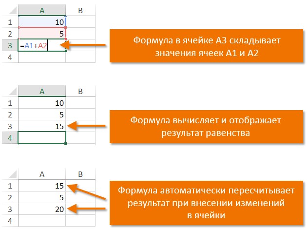
Все формулы в Excel должны начинаться со знака равенства (=). Это связано с тем, что Excel приравнивает данные хранящиеся в ячейке (т.е. формулу) к значению, которое она вычисляет (т.е. к результату).
Основные сведения о ссылках
Несмотря на то, что в Excel можно создавать формулы, применяя фиксированные значения (например, =2+2 или =5*5), в большинстве случаев для создания формул используются адреса ячеек. Этот процесс называется созданием ссылок. Создавая ссылки на ячейки убедитесь, что формулы не содержат ошибок.
Использование ссылок в формулах дает ряд преимуществ, начиная от меньшего количества ошибок и заканчивая простотой редактирования формул. К примеру, вы легко можете изменить значения, на которые ссылается формула, без необходимости ее редактировать.
Используя математические операторы, совместно со ссылками на ячейки, можно создать множество простых формул. На рисунке ниже приведены несколько примеров формул, которые используют разнообразные комбинации операторов и ссылок.
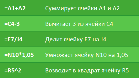
В Excel существует несколько видов ссылок. Изучите уроки раздела Относительные и абсолютные ссылки, чтобы получить дополнительную информацию.
Оцените качество статьи. Нам важно ваше мнение: