In excel what is a range of cells

A range is a group or block of cells in a worksheet that are selected or highlighted. Also, a range can be a group or block of cell references that are entered as an argument for a function, used to create a graph, or used to bookmark data.

Contiguous and Non-Contiguous Ranges

A contiguous range of cells is a group of highlighted cells that are adjacent to each other, such as the range C1 to C5 shown in the image above.

A non-contiguous range consists of two or more separate blocks of cells. These blocks can be separated by rows or columns as shown by the ranges A1 to A5 and C1 to C5.

Range Names

Ranges are so important in Excel and Google Spreadsheets that names can be given to specific ranges to make them easier to work with and reuse when referencing them in charts and formulas.

Select a Range in a Worksheet

When cells have been selected, they are surrounded by an outline or border. By default, this outline or border surrounds only one cell in a worksheet at a time, which is known as the active cell. Changes to a worksheet, such as data editing or formatting, affect the active cell.

When a range of more than one cell is selected, changes to the worksheet, with certain exceptions such as data entry and editing, affect all cells in the selected range.

There a number of ways to select a range in a worksheet. These include using the mouse, the keyboard, the name box, or a combination of the three.

To create a range consisting of adjacent cells, drag with the mouse or use a combination of the Shift and four arrow keys on the keyboard. To create ranges consisting of non-adjacent cells, use the mouse and keyboard or just the keyboard.

Select a Range for Use in a Formula or Chart

When entering a range of cell references as an argument for a function or when creating a chart, in addition to typing in the range manually, the range can also be selected using pointing.

Ranges are identified by the cell references or addresses of the cells in the upper left and lower right corners of the range. These two references are separated by a colon. The colon tells Excel to include all the cells between these start and endpoints.

Range vs. Array

At times the terms range and array seem to be used interchangeably for Excel and Google Sheets since both terms are related to the use of multiple cells in a workbook or file.

To be precise, the difference is because a range refers to the selection or identification of multiple cells (such as A1:A5) and an array refers to the values located in those cells (such as {1;2;5;4;3}).

Some functions, such as SUMPRODUCT and INDEX, take arrays as arguments. Other functions, such as SUMIF and COUNTIF, accept only ranges for arguments.

That’s not to say that a range of cell references cannot be entered as arguments for SUMPRODUCT and INDEX. These functions extract the values from the range and translate them into an array.

For example, the following formulas both return a result of 69 as shown in cells E1 and E2 in the image.

=SUMPRODUCT(A1:A5,C1:C5)
=SUMPRODUCT({1;2;5;4;3},{1;4;8;2;4})

On the other hand, SUMIF and COUNTIF do not accept arrays as arguments. So, while the formula below returns an answer of 3 (see cell E3 in the image), the same formula with an array would not be accepted.

COUNTIF(A1:A5,"<4")

As a result, the program displays a message box listing possible problems and corrections.

Thanks for letting us know!

---

Ranges

Range is an important part of Excel because it allows you to work with selections of cells.

There are four different operations for selection;

• Selecting a cell
• Selecting multiple cells
• Selecting a column
• Selecting a row

Before having a look at the different operations for selection, we will introduce the Name Box.

---

The Name Box

The Name Box shows you the reference of which cell or range you have selected. It can also be used to select cells or ranges by typing their values.

You will learn more about the Name Box later in this chapter.

---

Selecting a Cell

Cells are selected by clicking them with the left mouse button or by navigating to them with the keyboard arrows.

It is easiest to use the mouse to select cells.

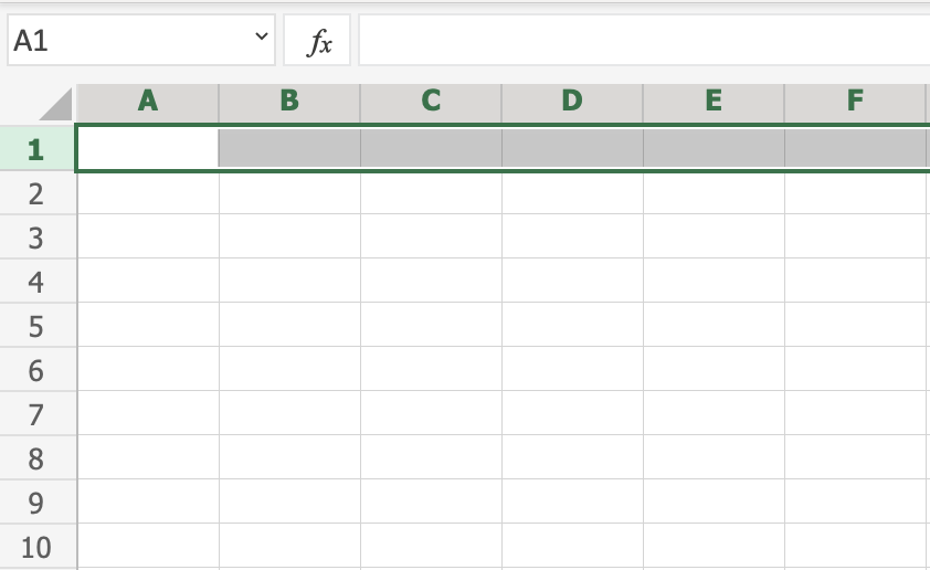
To select cell A1, click on it:

---

Selecting Multiple Cells

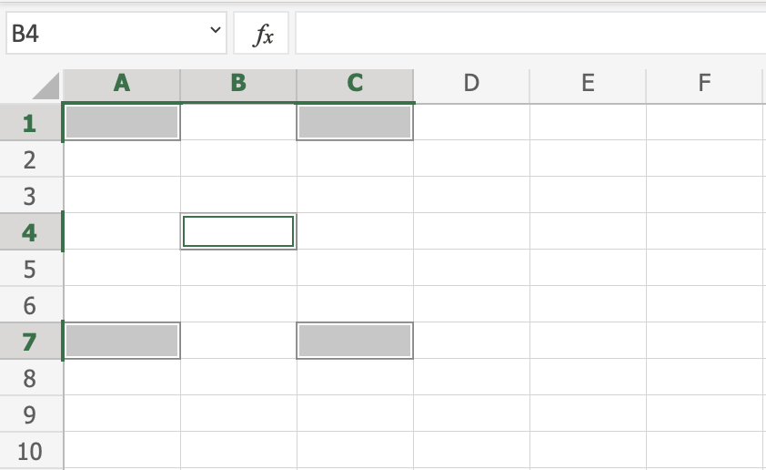
More than one cell can be selected by pressing and holding down CTRL or Command and left clicking the cells. Once finished with selecting, you can let go of CTRL or Command.

Lets try an example: Select the cells A1, A7, C1, C7 and B4.

Did it look like the picture below?

---

Selecting a Column

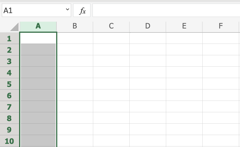
Columns are selected by left clicking it. This will select all cells in the sheet related to the column.

To select column A, click on the letter A in the column bar:

---

Selecting a Row

Rows are selected by left clicking it. This will select all the cells in the sheet related to that row.

To select row 1, click on its number in the row bar:

---

---

Selecting the Entire Sheet

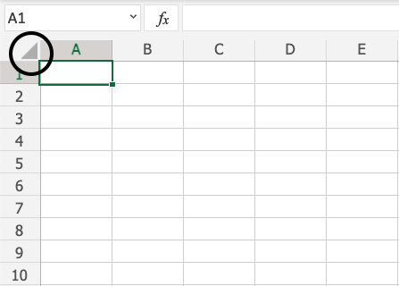
The entire spreadsheet can be selected by clicking the triangle in the top-left corner of the spreadsheet:

Now, the whole spreadsheet is selected:

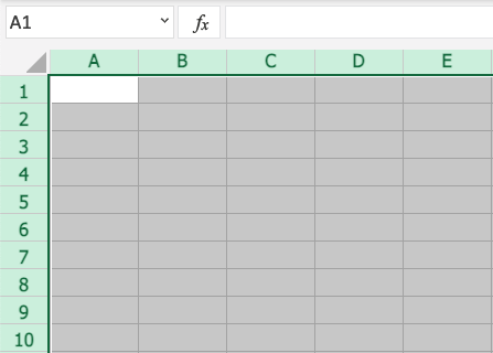
Note: You can also select the entire spreadsheet by pressing Ctrl+A for Windows, or Cmd+A for MacOS.

---

Selection of Ranges

Selection of cell ranges has many use areas and it is one of the most important concepts of Excel. Do not think too much about how it is used with values. You will learn about this in a later chapter. For now let’s focus on how to select ranges.

There are two ways to select a range of cells

1. Name Box
2. Drag to mark a range.

The easiest way is drag and mark. Let’s keep it simple and start there.

How to drag and mark a range, step-by-step:

1. Select a cell
2. Left click it and hold the mouse button down
3. Move your mouse pointer over the range that you want selected. The range that is marked will turn grey.
4. Let go of the mouse button when you have marked the range

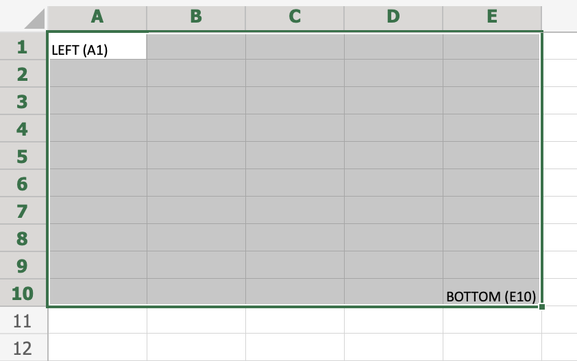
Let’s have a look at an example for how to mark the range A1:E10.

Note: You will learn about why the range is called A1:E10 after this example.

---

Select cell A1:

Press and hold A1 with the left mouse button. Move to the mouse pointer to mark the selection range. The grey area helps us to see the covered range.

Let go of the left mouse button when you have marked the range A1:E10:

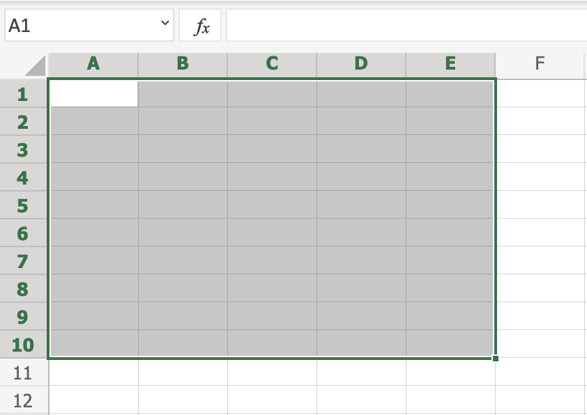
You have successfully selected the range A1:E10. Well done!

The second way to select a range is to enter the range values in the Name Box. The range is set by first entering the cell reference for the top left corner, then the bottom right corner. The range is made using those two as coordinates. That is why the cell range has the reference of two cells and the
: in between.

Top left corner reference : Right bottom corner reference

The range shown in the picture has the value of A1:E10:

The best way for now is to use the drag and mark method as it is easier and more visual.

In the next chapter you will learn about filling and how this applies to the ranges that we have just learned.

---

A range in Excel is nothing more than a set of adjacent cells that can be selected to perform the same operation on them. Because they are grouped, it is much easier to apply common formatting, sort items, or perform other spreadsheet tasks. Ranges are, in fact, the basis for many operations performed with the spreadsheet.

The full name of the set of cells is «range of cells», and is identified by the first and last cell in the set. For example, the range A1:C3 indicates that the two cells we have selected and on which operations can be performed are A1 and C3. We will be able to create graphs, insert functions, or form tables based on the data contained in these two cells.

To work with a range of cells, you can select them manually with the mouse, or you can type in the matrix just below the toolbar the range of cells you want to operate on following the formula above (the name of the start and end cell of the range separated by a colon).

It is worth remembering that Microsoft Excel is a software designed to work with spreadsheets. Its origins date back to 1983 when Microsoft introduced Multiplan as its own solution for this purpose. Later, when Lotus 1-2-3 was already dominating the spreadsheet market, it introduced the first version of Excel for Mac. It was 1985, and it would not be until 1987 that this software would appear for the first time in Windows. It is currently part of the Office package.