In excel range of numbers - Word и Excel - помощь в работе с программами

Explanation

Note: In Excel 365, the new SEQUENCE function is a better and easier way to create an array of numbers. The method explained below will work in previous versions.

The core of this formula is a string that represents rows. For example, to create an array with 10 numbers, you can hard-code a string into INDIRECT like this:

=ROW(INDIRECT("1:10"))

The INDIRECT function interprets this text to mean the range 1:10 (10 rows) and the ROW function returns the row number for each row in that range inside an array.

The example shown uses a more generic version of the formula that picks up the start and end numbers from B5 and C5 respectively, so the solution looks like this:

=ROW(INDIRECT(B5&":"&C5))
=ROW(INDIRECT(1&":"&5))
=ROW(INDIRECT("1:5"))
=ROW(1:5)
={1;2;3;4;5}

The reason INDIRECT is used in the formula is to guard against worksheet changes. Without INDIRECT, inserting or deleting rows can can change the range reference, for example:

=ROW(1:5)

will change to:

=ROW(1:4)

If row 1 is deleted. Because INDIRECT works with a reference constructed with text, it isn’t effected by changes on the worksheet.

Relative row numbers in a range

If you need an array that consists of the relative row numbers of a range, you can use a formula like this:

=ROW(range)-ROW(range.firstcell)+1

See this page for a full explanation.

Negative values

The ROW function won’t handle negative numbers, so you can’t mix negative numbers in for start and end. However, you can apply math operations to the array created by ROW. For example, the following formula will create this array: {-5;-4;-3;-2;-1}

=ROW(INDIRECT(1&":"&5))-6

Numbers in reverse order, n to 1

To create an array of positive numbers in descending order, from n to 1, you can use a formula like this:

=ABS(ROW(INDIRECT("1:"&n))-(n+1))

Источник

Excel 2021 for Mac Excel 2019 for Mac Excel 2016 for Mac Excel for Mac 2011 More…Less

Do any of the following.

In the column, type the first few characters for the entry.

If the characters that you type match an existing entry in that column, Excel presents a menu with a list of entries already used in the column.
Press the DOWN ARROW key to select the matching entry, and then press RETURN .
Notes:
- Excel automatically completes only those entries that contain text or a combination of text and numbers. Entries that contain only numbers, dates, or times are not completed.
- Entries that are repeated within a row are not included in the list of matching entries.
- If you don’t want the entries that you type to be matched automatically to other entries, you can turn this option off. On the Excel menu, click Preferences. Under Formulas and Lists, click AutoComplete , and then clear the Enable AutoComplete for cell values check box.

Select the cells that contain the data that you want to repeat in adjacent cells.
Drag the fill handle over the cells that you want to fill.

Note: When you select a range of cells that you want to repeat in adjacent cells, you can drag the fill handle down a single column or across a single row, but not down multiple columns and across multiple rows.

Click the Auto Fill Options smart button , and then do one of the following:

To	Do this
Copy the entire contents of the cell, including the formatting	Click Copy Cells.
Copy only the cell formatting	Click Fill Formatting Only.
Copy the contents of the cell, but not the formatting	Click Fill Without Formatting.

Notes:

To quickly enter the same information into many cells at once, select all of the cells, type the information that you want, and then press CONTROL + RETURN . This method works across any selection of cells.
If you don’t want the Auto Fill Options smart button to display when you drag the fill handle, you can turn it off. On the Excel menu, click Preferences. Under Authoring, click Edit , and then clear the Show Insert Options smart buttons check box.

Excel can continue a series of numbers, text-and-number combinations, or formulas based on a pattern that you establish. For example, you can enter Item1 in a cell, and then fill the cells below or to the right with Item2, Item3, Item4, etc.

Select the cell that contains the starting number or text-and-number combination.
Drag the fill handle over the cells that you want to fill.

Note: When you select a range of cells that you want to repeat in adjacent cells, you can drag the fill handle down a single column or across a single row, but not down multiple columns and across multiple rows.

Click the Auto Fill Options smart button , and then do one of the following:

To	Do this
Copy the entire contents of the cell, including the formulas and the formatting	Click Copy Cells.
Copy only the cell formatting	Click Fill Formatting Only.
Copy the contents of the cell, including the formulas but not the formatting	Click Fill Without Formatting.

Note: You can change the fill pattern by selecting two or more starting cells before you drag the fill handle. For example, if you want to fill the cells with a series of numbers, such as 2, 4, 6, 8…, type 2 and 4 in the two starting cells, and then drag the fill handle.

You can quickly fill cells with a series of dates, times, weekdays, months, or years. For example, you can enter Monday in a cell, and then fill the cells below or to the right with Tuesday, Wednesday, Thursday, etc.

Select the cell that contains the starting date, time, weekday, month, or year.
Drag the fill handle over the cells that you want to fill.

Note: When you select a range of cells that you want to repeat in adjacent cells, you can drag the fill handle down a single column or across a single row, but not down multiple columns and across multiple rows.

Click the Auto Fill Options smart button , and then do one of the following:

To	Do this
Copy the entire contents of the cell, including the formulas and the formatting, without repeating the series	Click Copy Cells.
Fill the cells based on the starting information in the first cell	Click Fill Series.
Copy only the cell formatting	Click Fill Formatting Only.
Copy the contents of the cell, including the formulas but not the formatting	Click Fill Without Formatting.
Use the starting date in the first cell to fill the cells with the subsequent dates	Click Fill Days.
Use the starting weekday name in the first cell to fill the cells with the subsequent weekdays (omitting Saturday and Sunday)	Click Fill Weekdays.
Use the starting month name in the first cell to fill the cells with the subsequent months of the year	Click Fill Months.
Use the starting date in the first cell to fill the cells with the date by subsequent yearly increments	Click Fill Years.

Note: You can change the fill pattern by selecting two or more starting cells before you drag the fill handle. For example, if you want to fill the cells with a series that skips every other day, such as Monday, Wednesday, Friday, etc., type Monday and Wednesday in the two starting cells, and then drag the fill handle.

Need more help?

You can always ask an expert in the Excel Tech Community or get support in the Answers community.

Need more help?

Источник

I have a table in Excel which looks like this:

             A             B           C
Row 1:    2100-2200    2200-2300    2300-2400

I’m using a VLOOKUP formula. I want this formula to find a number e.g. 2152 in the table above.

Cell A1 is supposed to contain numbers from 2100 to 2200.

Is this possible to do in Excel?

asked Feb 18, 2014 at 13:23

I dont know exactly what you want to return, this array formula will return the correct interval in A1:C1:

=INDEX($A$1:$C$1;MATCH(1;(E1>=VALUE(LEFT($A$1:$C$1;4)))*(E1<=VALUE(RIGHT($A$1:$C$1;4)));0))

Numeric value your looking for in E1

Dont forget to Ctrl Shift Enter to enter the formula…

answered Feb 18, 2014 at 13:48

CRondaoCRondao

1,8832 gold badges12 silver badges10 bronze badges

Instead of providing the ranges, you need to provide only the lower bound. I.e. try this data:

             A             B           C
Row 1:    2100          2200        2300

Because it is a horizontal setup, you need to use HLOOKUP (VLOOKUP will check the cells in the first column of a table, HLOOKUP the cells in the first row) — and you need to leave the fourth parameter of HLOOKUP/VLOOKUP blank (or set it to TRUE which is the same as leaving it blank). E.g. if you number 2152is in cell A2, use this formula:

=HLOOKUP(A2,$A$1:$C$1,1)

and you’ll get 2100.

If you want to have the full range returned, you should use the MATCH function instead:

=INDEX($A$1:$C$1,MATCH(A2,$A$1:$C$1))&"-"&INDEX($A$1:$C$1,MATCH(A2,$A$1:$C$1)+1)

This will return 2100-2200

answered Feb 18, 2014 at 13:49

Peter AlbertPeter Albert

16.8k4 gold badges66 silver badges88 bronze badges

use lower range of your numbers

                     A        B          C      D
Lower range        2100     2200       2300     2400
Ranking              1        2         3        4

You want to find a number or ranking corresponding to say 2350

Formula:   = HLOOKUP(2350,range (range of your values),2,TRUE)

your range includes 2100 -2400 plus 1-4.

the value 2 in the formula indicates the row that you want result returned from — in this case you want ranking — where 2350 will return a 4; change this number to 1 to return exact value.

sample formula:

= HLOOKUP(O65,J74:N75,2,TRUE)

answered Jul 18, 2015 at 0:09

As OP wants to apply HLookUp to numeric range strings ("2100-2200", "2200-2300", etc.), I suggest the following steps:

reconstruct the range contents to their starting values (2100,2200,2300) isolated via Find searching till the - delimiter) by VALUE(LEFT(A1:C1,FIND("-",A1:C1)-1))
define a named search cell MySrch (example value of 2151 due to OP) and apply HLookUp on the above values to get the lower boundary (here: 2100),
Match the found lower boundary (e.g. 2100) plus character "-" and a * wild card to find the ordinal column position (here: 1st column),
return the found range text (e.g. 2100-2200) via Index(A1:C1,1,{column number}) referring to row 1 and the column position as result:

   =INDEX(A1:C1,1,MATCH(HLOOKUP(MySrch,VALUE(LEFT(A1:C1,FIND("-",A1:C1)-1)),1)&"-*",A1:C1,0))

Note that it would be necessary to exclude search values outside the given range boundaries either by formula extension (e.g. If(MySrch>...,"?",{above formula}) or to add a last range defining a maximum limit.

answered Oct 7, 2021 at 18:28

T.M.T.M.

9,2293 gold badges32 silver badges57 bronze badges

if the number you search for is in E1 (aka e1 = 2152) then use 1 of 3:
the easiest and probably the best:

1) =HLOOKUP(E1 & "-" & E1,A1:C1,1,true)

2) =index(a1:c1,1, max(ARRAYFORMULA( if($E$1>VALUE(left(A1:C1,4)),column(A1:C1),0) )) )

3) =index(A1:c1,1, min(ARRAYFORMULA( if(VALUE(right(A1:C1,4))>=$E$1,column(A1:C1),99) )) )

this the range you want

to get the column remove the index(a1:c1,1, …. ) leaving the …. in 2) and 3) or use the fo;;owin gin 1)

=HLOOKUP(E1 & "-" & E1,{A1:C1 ; arrayformula(column(A1:C1))},2,true)

glad to help

answered Oct 7, 2021 at 19:49

Apostolos55Apostolos55

5743 silver badges8 bronze badges

Источник

I’m pretty sure this is not possible with a basic formula. However, I have also had this need before, and I wrote a worksheet function:

Public Function ConcatInts(target As Range) As String
    Dim s As String
    Dim i As Integer
    Dim n0 As Long
    Dim n1 As Long
    Dim n2 As Long
    Dim flag As Boolean
    n0 = 0
    n1 = target.Cells(1).Value
    n2 = n1
    flag = False
    For i = 2 To target.Cells.Count
        If IsNumeric(target.Cells(i).Value) Then
            n2 = target.Cells(i).Value
            If n2 = n1 + 1 Then
                If Not flag Then
                    n0 = n1
                    s = s & n1 & "-"
                    flag = True
                End If
            ElseIf n2 <> n1 Then
                If n1 = n0 + 1 And right(s, 1) = "-" Then
                    s = left(s, Len(s) - 1) & " "
                End If
                s = s & n1 & " "
                flag = False
            End If
            n1 = n2
        End If
    Next
    If n1 = n0 + 1 And right(s, 1) = "-" Then
        s = left(s, Len(s) - 1) & " "
    End If
    s = s & n1
    ConcatInts = s
End Function

To use this, you have to open up the VBA editor by pressing ALT+F11. Then right-click the workbook from the navigation pane and select Insert->Module:

Then just copy-paste the code into the module.

Now you can call it as you would a regular function:

=ConcatInts(A1:I1)

Note that this function skips over cells containing text, automatically converts floating-point numbers to integers, and discards duplicates. It also requires that your numbers be sorted.

Don’t forget to save your workbook as a macro-enabled workbook (XLSM).

Источник

Ranges

Range is an important part of Excel because it allows you to work with selections of cells.

There are four different operations for selection;

Selecting a cell
Selecting multiple cells
Selecting a column
Selecting a row

Before having a look at the different operations for selection, we will introduce the Name Box.

The Name Box

The Name Box shows you the reference of which cell or range you have selected. It can also be used to select cells or ranges by typing their values.

You will learn more about the Name Box later in this chapter.

Selecting a Cell

Cells are selected by clicking them with the left mouse button or by navigating to them with the keyboard arrows.

It is easiest to use the mouse to select cells.

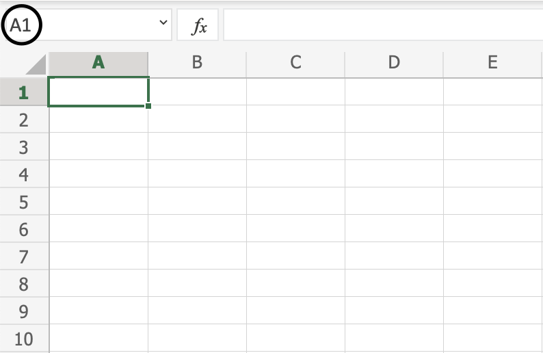
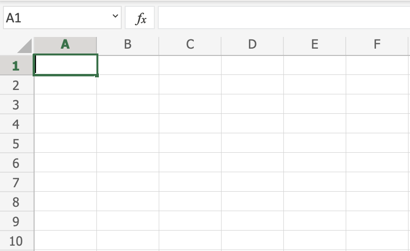
To select cell A1, click on it:

Selecting Multiple Cells

More than one cell can be selected by pressing and holding down CTRL or Command and left clicking the cells. Once finished with selecting, you can let go of CTRL or Command.

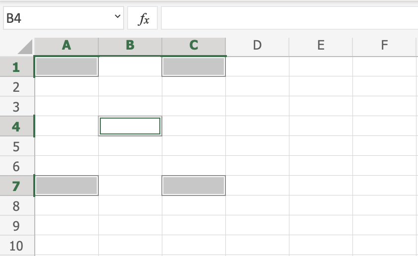
Lets try an example: Select the cells A1, A7, C1, C7 and B4.

Did it look like the picture below?

Selecting a Column

Columns are selected by left clicking it. This will select all cells in the sheet related to the column.

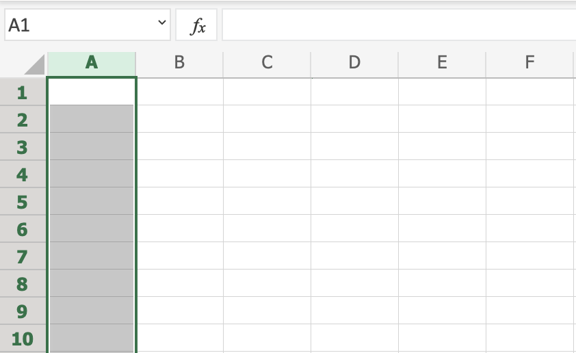
To select column A, click on the letter A in the column bar:

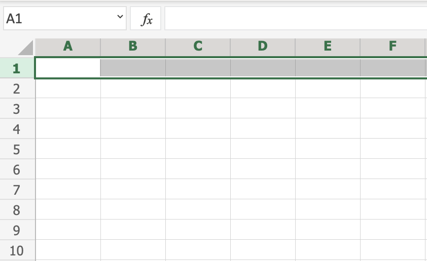
Selecting a Row

Rows are selected by left clicking it. This will select all the cells in the sheet related to that row.

To select row 1, click on its number in the row bar:

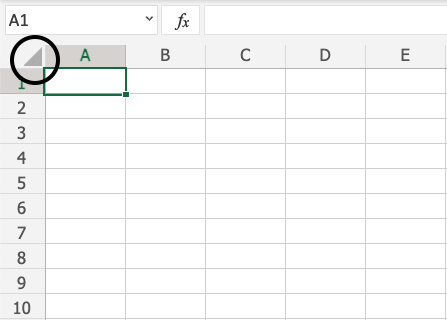
Selecting the Entire Sheet

The entire spreadsheet can be selected by clicking the triangle in the top-left corner of the spreadsheet:

Now, the whole spreadsheet is selected:

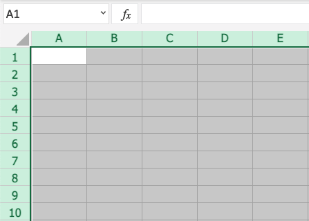
Note: You can also select the entire spreadsheet by pressing Ctrl+A for Windows, or Cmd+A for MacOS.

Selection of Ranges

Selection of cell ranges has many use areas and it is one of the most important concepts of Excel. Do not think too much about how it is used with values. You will learn about this in a later chapter. For now let’s focus on how to select ranges.

There are two ways to select a range of cells

Name Box
Drag to mark a range.

The easiest way is drag and mark. Let’s keep it simple and start there.

How to drag and mark a range, step-by-step:

Select a cell
Left click it and hold the mouse button down
Move your mouse pointer over the range that you want selected. The range that is marked will turn grey.
Let go of the mouse button when you have marked the range

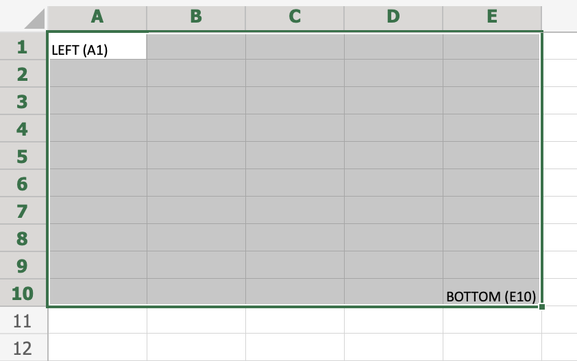
Let’s have a look at an example for how to mark the range A1:E10.

Note: You will learn about why the range is called A1:E10 after this example.

Select cell A1:

Press and hold A1 with the left mouse button. Move to the mouse pointer to mark the selection range. The grey area helps us to see the covered range.

Let go of the left mouse button when you have marked the range A1:E10:

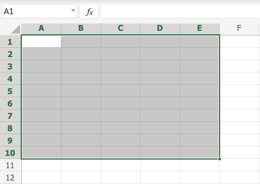
You have successfully selected the range A1:E10. Well done!

The second way to select a range is to enter the range values in the Name Box. The range is set by first entering the cell reference for the top left corner, then the bottom right corner. The range is made using those two as coordinates. That is why the cell range has the reference of two cells and the
: in between.

Top left corner reference : Right bottom corner reference

The range shown in the picture has the value of A1:E10:

The best way for now is to use the drag and mark method as it is easier and more visual.

In the next chapter you will learn about filling and how this applies to the ranges that we have just learned.

Test Yourself With Exercises

Источник

Explanation

Relative row numbers in a range

Negative values

Numbers in reverse order, n to 1

See also

Need more help?

Need more help?

Ranges

The Name Box

Selecting a Cell

Selecting Multiple Cells

Selecting a Column

Selecting a Row

Selecting the Entire Sheet

Selection of Ranges

Test Yourself With Exercises