In excel how do you move a column - Word и Excel - помощь в работе с программами

When you move or copy rows and columns, by default Excel moves or copies all data that they contain, including formulas and their resulting values, comments, cell formats, and hidden cells.

When you copy cells that contain a formula, the relative cell references are not adjusted. Therefore, the contents of cells and of any cells that point to them might display the #REF! error value. If that happens, you can adjust the references manually. For more information, see Detect errors in formulas.

You can use the Cut command or Copy command to move or copy selected cells, rows, and columns, but you can also move or copy them by using the mouse.

By default, Excel displays the Paste Options button. If you need to redisplay it, go to Advanced in Excel Options. For more information, see Advanced options.

Select the cell, row, or column that you want to move or copy.
Do one of the following:
- To move rows or columns, on the Home tab, in the Clipboard group, click Cut or press CTRL+X.
- To copy rows or columns, on the Home tab, in the Clipboard group, click Copy or press CTRL+C.
Right-click a row or column below or to the right of where you want to move or copy your selection, and then do one of the following:
- When you are moving rows or columns, click Insert Cut Cells.
- When you are copying rows or columns, click Insert Copied Cells.
Tip: To move or copy a selection to a different worksheet or workbook, click another worksheet tab or switch to another workbook, and then select the upper-left cell of the paste area.

Note: Excel displays an animated moving border around cells that were cut or copied. To cancel a moving border, press Esc.

By default, drag-and-drop editing is turned on so that you can use the mouse to move and copy cells.

Select the row or column that you want to move or copy.
Do one of the following:
- Cut and replace
  Point to the border of the selection. When the pointer becomes a move pointer , drag the rows or columns to another location. Excel warns you if you are going to replace a column. Press Cancel to avoid replacing.
- Copy and replace Hold down CTRL while you point to the border of the selection. When the pointer becomes a copy pointer , drag the rows or columns to another location. Excel doesn’t warn you if you are going to replace a column. Press CTRL+Z if you don’t want to replace a row or column.
- Cut and insert Hold down SHIFT while you point to the border of the selection. When the pointer becomes a move pointer , drag the rows or columns to another location.
- Copy and insert Hold down SHIFT and CTRL while you point to the border of the selection. When the pointer becomes a move pointer , drag the rows or columns to another location.
Note: Make sure that you hold down CTRL or SHIFT during the drag-and-drop operation. If you release CTRL or SHIFT before you release the mouse button, you will move the rows or columns instead of copying them.

Note: You cannot move or copy nonadjacent rows and columns by using the mouse.

If some cells, rows, or columns on the worksheet are not displayed, you have the option of copying all cells or only the visible cells. For example, you can choose to copy only the displayed summary data on an outlined worksheet.

Select the row or column that you want to move or copy.
On the Home tab, in the Editing group, click Find & Select, and then click Go To Special.
Under Select, click Visible cells only, and then click OK.
On the Home tab, in the Clipboard group, click Copy or press Ctrl+C. .
Select the upper-left cell of the paste area.

Tip: To move or copy a selection to a different worksheet or workbook, click another worksheet tab or switch to another workbook, and then select the upper-left cell of the paste area.
On the Home tab, in the Clipboard group, click Paste or press Ctrl+V.

If you click the arrow below Paste , you can choose from several paste options to apply to your selection.

Excel pastes the copied data into consecutive rows or columns. If the paste area contains hidden rows or columns, you might have to unhide the paste area to see all of the copied cells.

When you copy or paste hidden or filtered data to another application or another instance of Excel, only visible cells are copied.

Select the row or column that you want to move or copy.
On the Home tab, in the Clipboard group, click Copy or press Ctrl+C.
Select the upper-left cell of the paste area.
On the Home tab, in the Clipboard group, click the arrow below Paste , and then click Paste Special.
Select the Skip blanks check box.

Double-click the cell that contains the data that you want to move or copy. You can also edit and select cell data in the formula bar.
Select the row or column that you want to move or copy.
On the Home tab, in the Clipboard group, do one of the following:
- To move the selection, click Cut or press Ctrl+X.
- To copy the selection, click Copy or press Ctrl+C.
In the cell, click where you want to paste the characters, or double-click another cell to move or copy the data.
On the Home tab, in the Clipboard group, click Paste or press Ctrl+V.
Press ENTER.

Note: When you double-click a cell or press F2 to edit the active cell, the arrow keys work only within that cell. To use the arrow keys to move to another cell, first press Enter to complete your editing changes to the active cell.

When you paste copied data, you can do any of the following:

Paste only the cell formatting, such as font color or fill color (and not the contents of the cells).
Convert any formulas in the cell to the calculated values without overwriting the existing formatting.
Paste only the formulas (and not the calculated values).

Procedure

Select the row or column that you want to move or copy.
On the Home tab, in the Clipboard group, click Copy or press Ctrl+C.
Select the upper-left cell of the paste area or the cell where you want to paste the value, cell format, or formula.
On the Home tab, in the Clipboard group, click the arrow below Paste , and then do one of the following:
- To paste values only, click Values.
- To paste cell formats only, click Formatting.
- To paste formulas only, click Formulas.

When you paste copied data, the pasted data uses the column width settings of the target cells. To correct the column widths so that they match the source cells, follow these steps.

Select the row or column that you want to move or copy.
On the Home tab, in the Clipboard group, do one of the following:
- To move cells, click Cut or press Ctrl+X.
- To copy cells, click Copy or press Ctrl+C.
Select the upper-left cell of the paste area.

Tip: To move or copy a selection to a different worksheet or workbook, click another worksheet tab or switch to another workbook, and then select the upper-left cell of the paste area.
On the Home tab, in the Clipboard group, click the arrow under Paste , and then click Keep Source Column Widths.

You can use the Cut command or Copy command to move or copy selected cells, rows, and columns, but you can also move or copy them by using the mouse.

Select the cell, row, or column that you want to move or copy.
Do one of the following:
- To move rows or columns, on the Home tab, in the Clipboard group, click Cut or press CTRL+X.
- To copy rows or columns, on the Home tab, in the Clipboard group, click Copy or press CTRL+C.
Right-click a row or column below or to the right of where you want to move or copy your selection, and then do one of the following:
- When you are moving rows or columns, click Insert Cut Cells.
- When you are copying rows or columns, click Insert Copied Cells.
Tip: To move or copy a selection to a different worksheet or workbook, click another worksheet tab or switch to another workbook, and then select the upper-left cell of the paste area.

Note: Excel displays an animated moving border around cells that were cut or copied. To cancel a moving border, press Esc.

Select the row or column that you want to move or copy.
Do one of the following:
- Cut and insert
  Point to the border of the selection. When the pointer becomes a hand pointer , drag the row or column to another location
- Cut and replace Hold down SHIFT while you point to the border of the selection. When the pointer becomes a move pointer , drag the row or column to another location. Excel warns you if you are going to replace a row or column. Press Cancel to avoid replacing.
- Copy and insert Hold down CTRL while you point to the border of the selection. When the pointer becomes a move pointer , drag the row or column to another location.
- Copy and replace Hold down SHIFT and CTRL while you point to the border of the selection. When the pointer becomes a move pointer , drag the row or column to another location. Excel warns you if you are going to replace a row or column. Press Cancel to avoid replacing.
Note: Make sure that you hold down CTRL or SHIFT during the drag-and-drop operation. If you release CTRL or SHIFT before you release the mouse button, you will move the rows or columns instead of copying them.

Note: You cannot move or copy nonadjacent rows and columns by using the mouse.

Double-click the cell that contains the data that you want to move or copy. You can also edit and select cell data in the formula bar.
Select the row or column that you want to move or copy.
On the Home tab, in the Clipboard group, do one of the following:
- To move the selection, click Cut or press Ctrl+X.
- To copy the selection, click Copy or press Ctrl+C.
In the cell, click where you want to paste the characters, or double-click another cell to move or copy the data.
On the Home tab, in the Clipboard group, click Paste or press Ctrl+V.
Press ENTER.

Note: When you double-click a cell or press F2 to edit the active cell, the arrow keys work only within that cell. To use the arrow keys to move to another cell, first press Enter to complete your editing changes to the active cell.

When you paste copied data, you can do any of the following:

Paste only the cell formatting, such as font color or fill color (and not the contents of the cells).
Convert any formulas in the cell to the calculated values without overwriting the existing formatting.
Paste only the formulas (and not the calculated values).

Procedure

Select the row or column that you want to move or copy.
On the Home tab, in the Clipboard group, click Copy or press Ctrl+C.
Select the upper-left cell of the paste area or the cell where you want to paste the value, cell format, or formula.
On the Home tab, in the Clipboard group, click the arrow below Paste , and then do one of the following:
- To paste values only, click Paste Values.
- To paste cell formats only, click Paste Formatting.
- To paste formulas only, click Paste Formulas.

You can move or copy selected cells, rows, and columns by using the mouse and Transpose.

Select the cells or range of cells that you want to move or copy.
Point to the border of the cell or range that you selected.
When the pointer becomes a , do one of the following:

To	Do this
Move cells	Drag the cells to another location.
Copy cells	Hold down OPTION and drag the cells to another location.

Note: When you drag or paste cells to a new location, if there is pre-existing data in that location, Excel will overwrite the original data.

Select the rows or columns that you want to move or copy.
Point to the border of the cell or range that you selected.
When the pointer becomes a , do one of the following:

To	Do this
Move rows or columns	Drag the rows or columns to another location.
Copy rows or columns	Hold down OPTION and drag the rows or columns to another location.
Move or copy data between existing rows or columns	Hold down SHIFT and drag your row or column between existing rows or columns. Excel makes space for the new row or column.

Copy the rows or columns that you want to transpose.
Select the destination cell (the first cell of the row or column into which you want to paste your data) for the rows or columns that you are transposing.
On the Home tab, under Edit, click the arrow next to Paste, and then click Transpose.

Note: Columns and rows cannot overlap. For example, if you select values in Column C, and try to paste them into a row that overlaps Column C, Excel displays an error message. The destination area of a pasted column or row must be outside the original values.

Things You Should Know

On Windows or Mac, select the column, then click and drag the border of the selection to a new location.
On Windows, select the column, then press Ctrl + x to cut the column. Right-click the column to the right of the new destination and select “Insert Cut Cells.”
To move multiple adjacent columns, press Ctrl (Windows) or Cmd (macOS). Then, click the column letters above the columns you want to move.

1
Click the letter above the column you want to move. This selects the column. In this method, you’ll use the mouse to drag the column to a new position. This works on Windows and macOS.
- This method only works for a single column. To move multiple columns, use cut and paste commands (see next method).
- Moving columns is a great way to set up your spreadsheet for a Vlookup or Sum formula.
- For general spreadsheet tips, check out our guide on making a spreadsheet in Excel.
2
Hover the mouse over the border of the selected column. The cursor will turn into four arrows (Windows) or a hand (macOS).^[1]
- The cursor will turn into a hand in the web app version of Excel.
Advertisement
3
Drag the column to the desired location. Click and drag the selected column to the location where you want to move it, and then release the mouse button. This will cut and replace the column.
- If you want to copy and replace columns instead of just moving them, hold down Ctrl (Windows) or ⌥ Option (macOS) while dragging and dropping.
- Holding ⇧ Shift will cut and insert the columns.
- Holding Ctrl+⇧ Shift will copy and insert the columns.

1
Click the letter above the column you want to move. This selects the column. The commands method only works on the Windows version of Excel.
- To move more than one (adjacent) column at the same time, hold down Ctrl as you click each column letter.
- Formatting your spreadsheet can significantly improve your Excel experience.
2
Press Ctrl+X. This “cuts” the data in the column, which really just selects it and adds it to the clipboard.
- The column data will remain in its place until you paste it into its new location.
- You can also cut the column by clicking the scissors icon on the Home tab. It’s in the “Clipboard” section near the top-left corner of the app.
- If you cut the wrong column, press Esc to return the data to its original location.
3
Right-click the letter above the column to the right of where you want to move the data. A drop-down menu will open.
- When you insert your copied data, it’ll be to the left of the column you right-click.
4
Click Insert Cut Cells on the right-click menu. Excel will insert the cut column to the left of the one on which you right-clicked.
- If you want to undo the pasted column, press Ctrl+Z.
- Alternatively, you can click the drop-down icon next to the Insert button on the Home toolbar at the top, and select Insert Cut Cells or Insert Cells here. This will insert and move your data the same way.

Add New Question

Question

columns a and b suddenly disappeared from excel. how to retrieve?

Kyle Smith is a wikiHow Technology Writer, learning and sharing information about the latest technology. He has presented his research at multiple engineering conferences and is the writer and editor of hundreds of online electronics repair guides. Kyle received a BS in Industrial Engineering from Cal Poly, San Luis Obispo.

wikiHow Technology Writer

Expert Answer

The columns might be hidden! Try selecting the adjacent column (c) and right-clicking that column. Select Unhide from the pop-up menu.
Question

see column B and K at the same time

Kyle Smith is a wikiHow Technology Writer, learning and sharing information about the latest technology. He has presented his research at multiple engineering conferences and is the writer and editor of hundreds of online electronics repair guides. Kyle received a BS in Industrial Engineering from Cal Poly, San Luis Obispo.

wikiHow Technology Writer

Expert Answer

There are a few ways to go about this! You can freeze columns A and B to keep them on the screen at all times. Alternatively, hide some or all columns between B and K so that they’re closer together. You could also move column K next to B using this guide’s method above.

Ask a Question

200 characters left

Include your email address to get a message when this question is answered.

Submit

Looking for money-saving deals on Microsoft Office products like Excel? Check out our coupon site for tons of coupons and promo codes on your next subscription.

Thanks for submitting a tip for review!

About This Article

Article SummaryX

1. Click the column letter.
2. Hover the mouse over the selection’s edge until the cursor changes.
3. Click and drag the column to a different location.

Did this summary help you?

Thanks to all authors for creating a page that has been read 190,819 times.

Is this article up to date?

Источник

There are three ways to move a column; the easiest is to highlight and drag-and-drop the column where you want it

Updated on November 12, 2022

What to Know

The easiest way to move a column in Excel is to highlight it, press Shift, and drag it to the new location.
You can also use cut & paste or do Data Sort to rearrange columns from the Data tab.
Columns that are part of a merged group of cells will not move.

This article covers how to move a column in Excel using the mouse, cut and paste a column, and rearrange columns using the Data Sort function. These instructions apply to Microsoft Excel 2019 and 2016 as well as Excel in Office 365.

Move Columns Using Your Mouse

There are several ways to rearrange the columns in an Excel worksheet, but one is easier than all the others. It just takes a highlight and a drag-and-drop motion. Here’s how to move columns in Excel using your mouse.

In the worksheet where you want to rearrange columns, place your cursor over the top of the column you want to move. You should see your cursor change to an arrow. When it does, click to highlight the column.
Next, press and hold the Shift key on the keyboard and then click and hold on the right or left border of the column you want to move and drag it to the right or left.

As you drag your cursor across the columns, you’ll see the borders darken to indicate where the new column will appear. When you’re happy with the location, release the mouse click.
You column will be moved to the location indicated by the darker border.

Move a Column in Excel With Cut and Paste

The next easiest way to move a column in Excel is to cut and paste the column from the old location to the new. This works much as you would expect it.

Highlight the column you want to move, and then press Ctrl + X on your keyboard to cut the column from its current location. You’ll see the «marching ants» around the column to indicate it has been cut from its current location.
Next, highlight a column to the right of where you want to move the cut column to, and right-click. In the menu, select Insert Cut Cells.
The new column is inserted to the left of the selected column.

Move Columns Using a Data Sort

Moving columns with a data sort is probably not the easiest way to move things around if you only have one or two columns that need to be moved, but if you have a large spreadsheet and you want to change the order of numerous columns, this little trick could be a major time saver.

This method will not work if you have Data Validation in place on your existing columns. To proceed, you’ll need to remove data validation. To do so, highlight the cells with data validation, select Data Validation > Settings > Clear All, and click OK.

To start, you need to add a row to the very top of your spreadsheet. To do this, right-click the first row and select Insert from the context menu.
A new row is inserted above your top row. This row must be at the top of the page, above all other header rows or rows of information.

Go through your spreadsheet and number the columns in the order you want them to appear in the spreadsheet by entering a number in the new top row. Be sure to number every column you’re using.
Next, select all the data in the spreadsheet that you want to rearrange. Then on the Data tab, in the Sort & Filter group, click Sort.
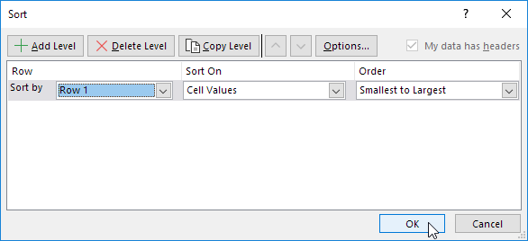
In the Sort dialog box, click Options.
In the Sort Options dialog box, click the radio button next to Sort left to right and then click OK.
You’re returned to the Sort dialog box. In the Sort By drop down menu select Row 1 and then click OK.
This should sort your columns according to the numbers you listed in that first row. Now you can right click the first row and select Delete to get rid of it.

FAQ

How do I unhide columns in Excel?

To unhide any single column in Excel, use the keyboard shortcut Ctrl+Shift+0. (You must select at least one column on either side of a hidden column or columns to unhide them.) You can also go to the Home tab > Cells group, select Format > Visibility > Hide & Unhide, and then select Unhide Columns.
How do I add columns in Excel?

To add columns in Excel, right-click the top of the column and select Insert. You can also go to the Home tab > Cells group and select Insert > Insert Sheet Columns.
How do I combine two columns in Excel?

To combine two columns in Excel, insert a new column near the two columns (A2 and B2 in this example) you want to combine. Select the first cell below the heading of the new column (C2) and enter =CONCATENATE(A2,» «,B2) into the formula bar. This combines the data in cell A2 with the data in cell B2, with a space between them.

Thanks for letting us know!

Get the Latest Tech News Delivered Every Day

Источник

Содержание

Move Columns
Shift Key
Insert Cut Cells
Magic Move
How to Move Columns in Excel
In This Article
What to Know
Move Columns Using Your Mouse
Move a Column in Excel With Cut and Paste
Move Columns Using a Data Sort
How to swap columns by dragging and other ways to move columns in Excel
How to drag columns in Excel
Swap Excel columns by cutting and pasting
How to move one column in Excel
How to move several columns in Excel
Swap multiple columns by copying, pasting and deleting
Change the columns order in Excel using VBA
Re-arrange columns with Column Manager

Move Columns

To move columns in Excel, use the shift key or use Insert Cut Cells. You can also change the order of all columns in one magic move.

Shift Key

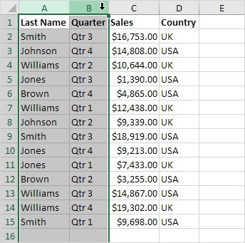
To quickly move columns in Excel without overwriting existing data, press and hold the shift key on your keyboard.

1. First, select a column.

2. Hover over the border of the selection. A four-sided arrow appears.

3. Press and hold the Shift key on your keyboard.

4. Click and hold the left mouse button.

5. Move the column to the new position.

6. Release the left mouse button.

7. Release the shift key.

To move multiple columns in Excel without overwriting existing data.

8. First, select multiple columns by clicking and dragging over the column headers.

9. Repeat steps 2-7.

Note: in a similar way, you can move a single row or multiple rows in Excel.

Insert Cut Cells

If you prefer the old-fashioned way, execute the following steps.

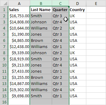
1. First, select a column.

2. Right click, and then click Cut.

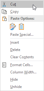
3. Select a column. The column will be inserted before the selected column.

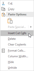
4. Right click, and then click Insert Cut Cells.

Note: in a similar way, you can move multiple columns, a single row or multiple rows.

Magic Move

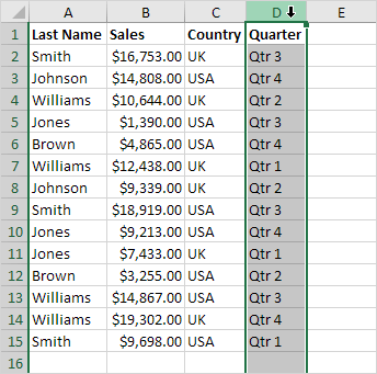
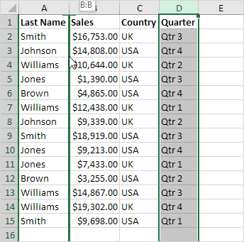
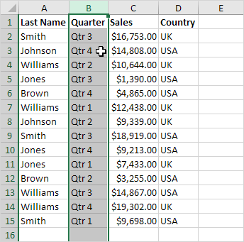
Finally, you can change the order of all columns in one magic move. Are you ready?

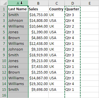
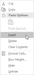
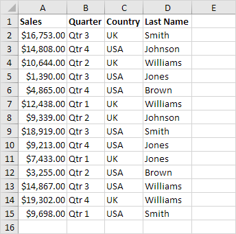
2. Right click, and then click Insert.

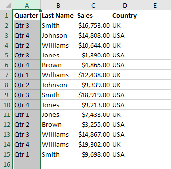
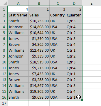
3. Use the first row to indicate the new order of the columns (Sales, Quarter, Country, Last Name).

4. Select the data.

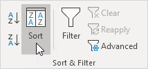
5. On the Data tab, in the Sort & Filter group, click Sort.

The Sort dialog box appears.

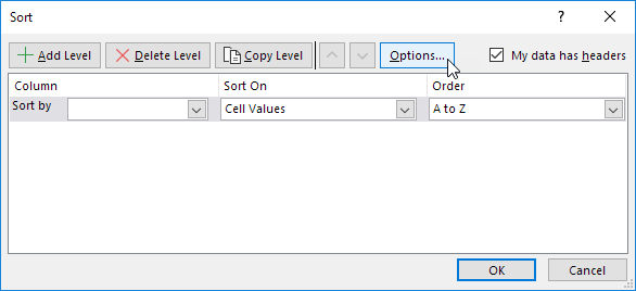
6. Click Options.

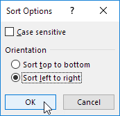
7. Click Sort left to Right and click OK.

8. Select Row 1 from the ‘Sort by’ drop-down list and click OK.

Note: this technique is pretty impressive if you need to rearrange the order of many columns.

Источник

How to Move Columns in Excel

There are three ways to move a column; the easiest is to highlight and drag-and-drop the column where you want it

What to Know

The easiest way to move a column in Excel is to highlight it, press Shift, and drag it to the new location.
You can also use cut & paste or do Data Sort to rearrange columns from the Data tab.
Columns that are part of a merged group of cells will not move.

Move Columns Using Your Mouse

In the worksheet where you want to rearrange columns, place your cursor over the top of the column you want to move. You should see your cursor change to an arrow. When it does, click to highlight the column.

Next, press and hold the Shift key on the keyboard and then click and hold on the right or left border of the column you want to move and drag it to the right or left.

As you drag your cursor across the columns, you’ll see the borders darken to indicate where the new column will appear. When you’re happy with the location, release the mouse click.

You column will be moved to the location indicated by the darker border.

Move a Column in Excel With Cut and Paste

The next easiest way to move a column in Excel is to cut and paste the column from the old location to the new. This works much as you would expect it.

Highlight the column you want to move, and then press Ctrl + X on your keyboard to cut the column from its current location. You’ll see the «marching ants» around the column to indicate it has been cut from its current location.

Next, highlight a column to the right of where you want to move the cut column to, and right-click. In the menu, select Insert Cut Cells.

The new column is inserted to the left of the selected column.

Move Columns Using a Data Sort

To start, you need to add a row to the very top of your spreadsheet. To do this, right-click the first row and select Insert from the context menu.

A new row is inserted above your top row. This row must be at the top of the page, above all other header rows or rows of information.

Go through your spreadsheet and number the columns in the order you want them to appear in the spreadsheet by entering a number in the new top row. Be sure to number every column you’re using.

Next, select all the data in the spreadsheet that you want to rearrange. Then on the Data tab, in the Sort & Filter group, click Sort.

In the Sort dialog box, click Options.

In the Sort Options dialog box, click the radio button next to Sort left to right and then click OK.

You’re returned to the Sort dialog box. In the Sort By drop down menu select Row 1 and then click OK.

This should sort your columns according to the numbers you listed in that first row. Now you can right click the first row and select Delete to get rid of it.

To unhide any single column in Excel, use the keyboard shortcut Ctrl+Shift+0. (You must select at least one column on either side of a hidden column or columns to unhide them.) You can also go to the Home tab > Cells group, select Format > Visibility > Hide & Unhide, and then select Unhide Columns.

To add columns in Excel, right-click the top of the column and select Insert. You can also go to the Home tab > Cells group and select Insert > Insert Sheet Columns.

To combine two columns in Excel, insert a new column near the two columns (A2 and B2 in this example) you want to combine. Select the first cell below the heading of the new column (C2) and enter =CONCATENATE(A2,» «,B2) into the formula bar. This combines the data in cell A2 with the data in cell B2, with a space between them.

Источник

How to swap columns by dragging and other ways to move columns in Excel

by Svetlana Cheusheva, updated on February 7, 2023

In this article, you will learn a few methods to swap columns in Excel. You will see how to drag columns with a mouse and how to move a few non-contiguous columns at a time. The latter is often considered unfeasible, but in fact there’s a tool that allows moving non-adjacent columns in Excel 2016, 2013 and 2010 in a click.

If you extensively use Excel tables in your daily work, you know that whatever logical and well thought-out a table’s structure is, you have to reorder the columns every now and then. For example, you might need to swap a couple of columns to view their data side-by-side. Of course, you can try to hide the neighboring columns for a while, however this is not always the best approach because you may need to see data in those columns as well.

Surprisingly, Microsoft Excel does not provide a straightforward way to perform this common operation. If you try to simply drag a column name, which appears to be the most obvious way to move columns, you might be confused to find that it does not work.

All in all, there are four possible ways to switch columns in Excel, namely:

How to drag columns in Excel

As already mentioned, dragging columns in Excel is a bit more complex procedure than one could expect. In fact, it’s one of those cases that can be classified as «easier said than done». But maybe it’s just my lack of sleight of hand ability 🙂 Nevertheless, with some practice, I was able to get it to work, so you will definitely manage it too.

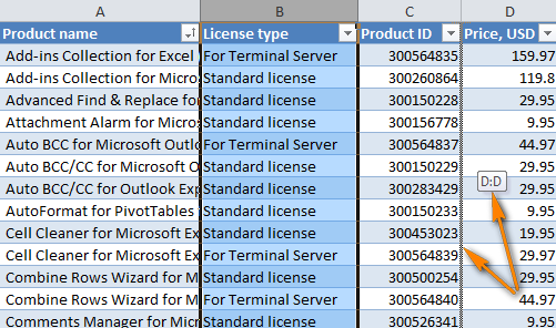
Suppose, you have a worksheet with information about your company’s products and you want to quickly swap a couple of columns there. I will use the AbleBits price list for this example. What I want is to switch the «License type» and «Product ID» columns so that a product ID comes right after the product name.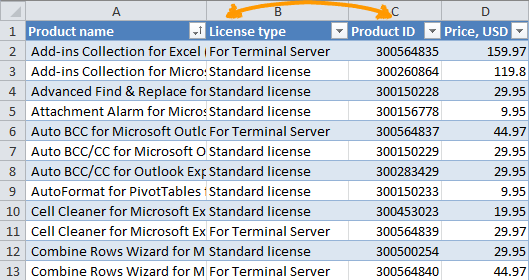

Select the column you want to move.
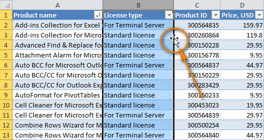
Put the mouse pointer to the edge of the selection until it changes from a regular cross to a 4-sided arrow cursor. You’d better not do this anywhere around the column heading because the cursor can have too many different shapes in that area. But it works just fine on the right or left edge of the selected column, as shown in the screenshot.
Press and hold the Shift key, and then drag the column to a new location. You will see a faint «I» bar along the entire length of the column and a box indicating where the new column will be moved.
That’s it! Release the mouse button, then leave the Shift key and find the column moved to a new position.

You can use the same technique to drag several columns in your Excel table. To select several columns, click the heading of the first column you need to move, press and hold Shift , and then click the heading of the last column. Then follow steps 2 — 4 above to move the columns, as shown in the screenshot.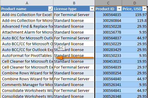

Note. It is not possible to drag non-adjacent columns and rows in Excel.

The drag and drop method works in Microsoft Excel 2016, 2013, 2010 and 2007 and can be used for moving rows as well. It might require some practice, but once mastered it could be a real time saver. Though, I guess the Microsoft Excel team will hardly ever win an award for the most user friendly interface on this feature 🙂

Swap Excel columns by cutting and pasting

If manipulating the mouse pointer is not your technique of choice, then you can change the columns order by cutting and pasting them. Please keep in mind that there’re a few tricks here depending on whether you want to move a single column or several columns at a time:

How to move one column in Excel

Select the entire column by clicking on the column header.
Cut the selected column by pressing Ctlr + X , or right click the column and choose Cut from the context menu. You can actually skip step 1 and simply right click the column’s heading to choose Cut.
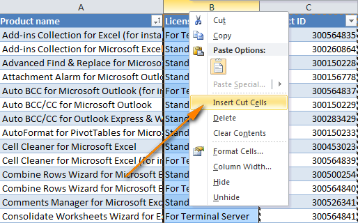
Select the column before which you want to insert the cut column, right click it and choose Insert Cut Cells from the pop-up menu.

If you are more comfortable with Excel shortcuts and keyboard, then you may like the following way to move columns in Excel:

Select any cell in the column and press Ctrl + Space to select the whole column.
Hit Ctrl + X to cut the column.
Select the column before which you what to paste the cut column.
Press Ctrl together with the Plus sign (+) on the numeric keypad to insert the column.

How to move several columns in Excel

The cut / paste method that works just fine for a single column does not allow switching several columns at a time. If you try to do this, you will end up with the following error: The command you chose cannot be performed with multiple selections.

To reorder a few columns in your worksheet, choose one of the following options:

Drag several columns using the mouse (in my opinion, this is the fastest way).
Cut and paste each column individually (probably not the best approach if you have to move a lot of columns).
Copy, paste and delete (allows moving several adjacent columns at a time).

Swap multiple columns by copying, pasting and deleting

If dragging columns with a mouse does not work for you for some reason, then you can try to re-arrange several columns in your Excel table is this way:

Select the columns you want to switch (click the first column’s heading, press Shift and then click the last column heading).

An alternative way is to select only the headings of the columns to be moved and then press Ctrl + Space . This will select only cells with data rather than entire columns, as shown in the screenshot below.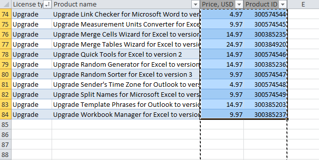

Note. If you are re-arranging columns in a range, either way will do. If you are to swap a few columns in an Excel table, then select the columns using the second way (cells with data only), otherwise you may get the error «The operation is not allowed. The operation is attempting to shift cells in a table of your worksheet».

Of course, this is a bit longer process compared to dragging columns, but it may work for those who prefer shortcuts to fiddling with the mouse. Regrettably, it does not work for non-contingent columns either.

Change the columns order in Excel using VBA

If you have some knowledge of VBA, you can try to write a macro that would automate moving columns in your Excel sheets. This is in theory. In practice, most likely you would end up spending more time on specifying which exactly columns to swap and defining their new placements than dragging the columns manually. Besides, there is no guarantee that the macro will always work as expected and each time you would need to verify the result anyways. All in all, a VBA macro does not seem to be well-suited for this task.

Re-arrange columns with Column Manager

If you are looking for a fast and reliable tool to switch columns in your Excel sheets, the Column Manager included with our Ultimate Suite is certainly worth your attention. It lets you change the order of columns on the fly, without manual copying / pasting or learning a handful of shortcuts.

With the Ultimate Suite installed in your Excel, click the Colum Manager button on the Ablebits Data tab, in the Manage group: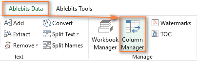

The Column Manager’s pane will appear in the right side of the Excel window and displays a list of columns that are present in your active worksheet.

To move one or more columns, select them on the pane and click the Up or Down arrow on the toolbar. The former moves the selected columns to the left in your sheet, the latter to the right: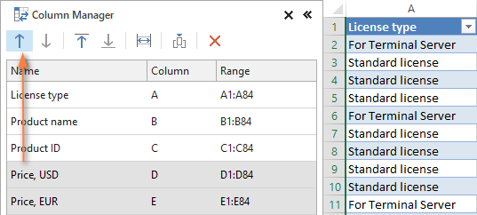

Or, drag-and-drop the columns on the pane with your mouse. Both methods work for adjacent and non-adjacent columns: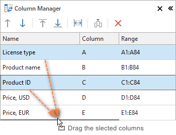

All the manipulations that you do on the Colum Manager pane are simultaneously performed on your worksheet, which lets you visually see all the changes and have full control over the process.

Another truly wonderful feature is the ability to move a single column or multiple columns to the beginning (far left) or to the end (far right) of the table in a click: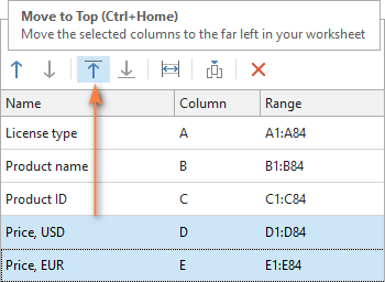

And finally, a couple of nice bonuses:
— Click this icon to auto fit the width of the selected columns.

— Click this icon to insert a new column.

I have to admit that I really love this little smart add-in. Together with the other 70+ tools included in the Ultimate Suite, it makes common operations in Excel not only faster and easier, but actually enjoyable. Of course, you should not take my words for granted because I’ve got used to them and therefore am sort of biased 🙂

So, go ahead and download a trial version to see for yourself.

Источник

By properly arranging the columns in a spreadsheet, you can make it easier to read and find specific data. Here are some simple ways you can do it.

The arrangement of columns and rows in an Excel spreadsheet is an important factor in its readability and convenience. Sometimes you need to improve your spreadsheet by moving the columns in your Excel spreadsheet.

Manually entering the data in a column to another column might be the go-to solution if the column includes few cells, but this method will be excruciating in larger columns. Luckily, there are methods that allow you to effortlessly move columns in Excel.

1. Move Columns With Drag and Drop

The easiest way to move columns in Excel is by dragging and dropping them where you want.

Select the column you want to move. You can do this by clicking the column heading (for example, the letter B).
Hold Shift and grab the right or left border of the column.
Drop the column into the new position. Notice that as you’re moving the column around, some borders on the spreadsheet will be highlighted to indicate where the column will be placed.

This trick isn’t exclusive to columns, and you can use it to move rows or any group of cells as well. All you need to do is to select them and then drag and drop them with Shift held down.

2. Move Columns With Cut and Paste

Another easy method is cutting and pasting the column to a new position. To do this, all you need is to cut the column’s content and then paste it into a new column.

Select the column that you want to move.
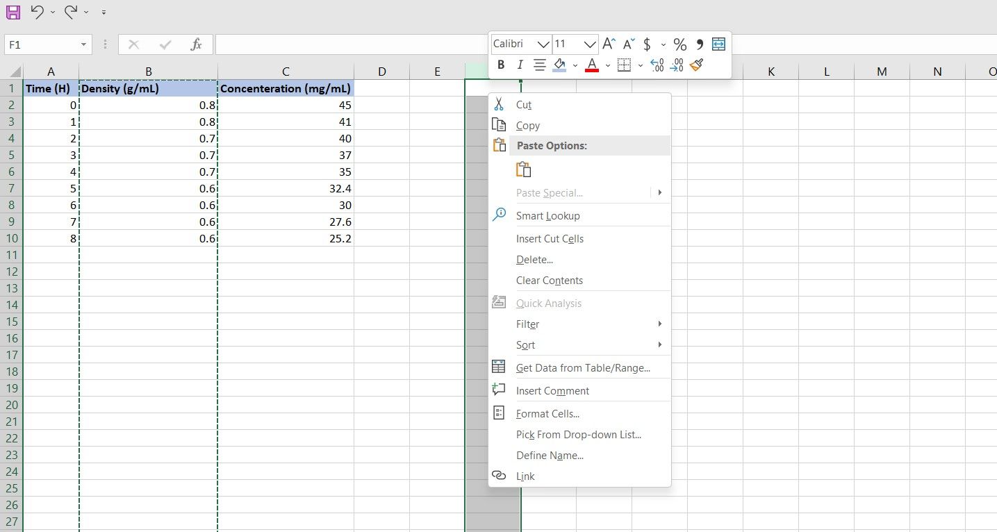
Press Ctrl + X on your keyboard. You can also right-click on the selected columns and select Cut. The cut column will have a dotted highlight.
Select the target column.
Press Ctrl + P on your keyboard to paste the column’s content. You can also right-click on the column to use the Paste Option.

3. Move Columns With Data Sort

This method is a bit more complex than the previous ones, but it pays well if you want to move a large spreadsheet with lots of columns. Using Data Sort to move columns lets you move multiple columns at once.

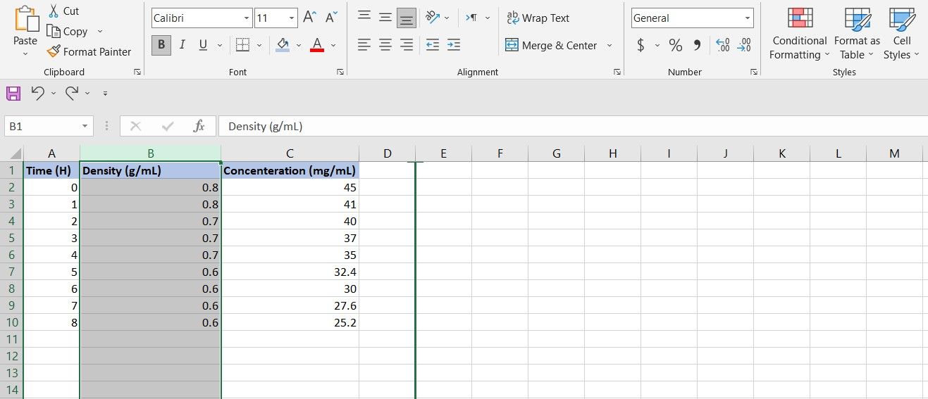
To use Data Sort to move columns, you need to add a row to the beginning of your spreadsheet and indicate the sorting order there. Then you can sort the columns with Data Sort.

Right-click a cell in the first row and then select Insert. This will insert a row on top of the first row.
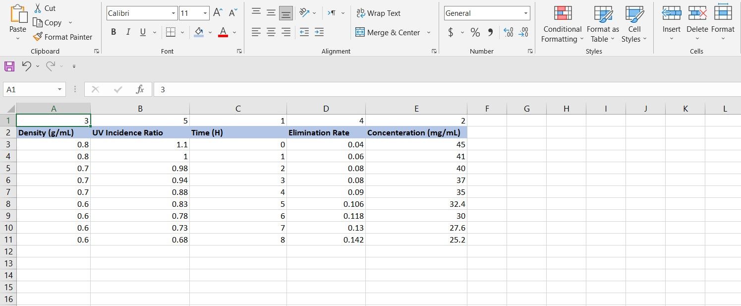
In the new row, insert the sorting order for your columns on top of each column. For instance, if you want the first column to be the fourth column in the new order, type a 4 in the cell above it.
Select the entire data table.
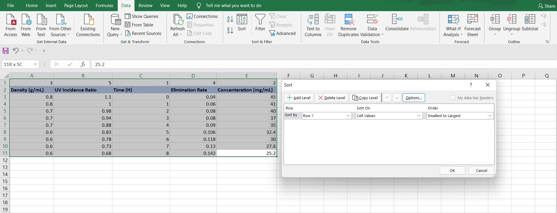
Go to the Data menu and select Sort from the Sort & Filter section. The Sort window will open.
In the Sort window, click Options.
Under Orientation, check Sort left to right.
Select OK.
Now back in the Sort window, select Row 1 in the Sort by menu. This will sort your table by the first row, where you put the numbers.
Select Cell Values under Sort on. This will sort the columns based on the values in the first row.
Select Smallest to Largest for Order. This way, the column numbered 1 will be first, and the others will come after it in sequence.
Finally, when everything is set, click OK.

Now you have your columns moved to the position you wanted. There remains a slight inconvenience, and that is the first row. Let’s get rid of that.

Right-click on a cell in the first row.
From the menu, select Delete. A window will appear asking you what you want to delete.
Check Entire row and click OK.

Your data table is all sorted the way you wanted it now. If you’re dealing with dates in your data table and want to sort them, you should read our article on how to sort by date in Excel.

4. Move Columns With the SORT Function

If you want to rearrange your columns without losing the original arrangement, the SORT function lets you do this.

With the SORT function, you can make a rearranged copy of your data table, while keeping the original table intact. This way, you can rearrange and move the columns in a data table in one act, and then delete the old table if you’re happy with the new one.

The SORT function syntax is as below:

=SORT(array, sort_index, sort_order, by_column)

Using SORT to move columns is similar to using Data Sort, except that it is done through a function, and the original table won’t be changed.

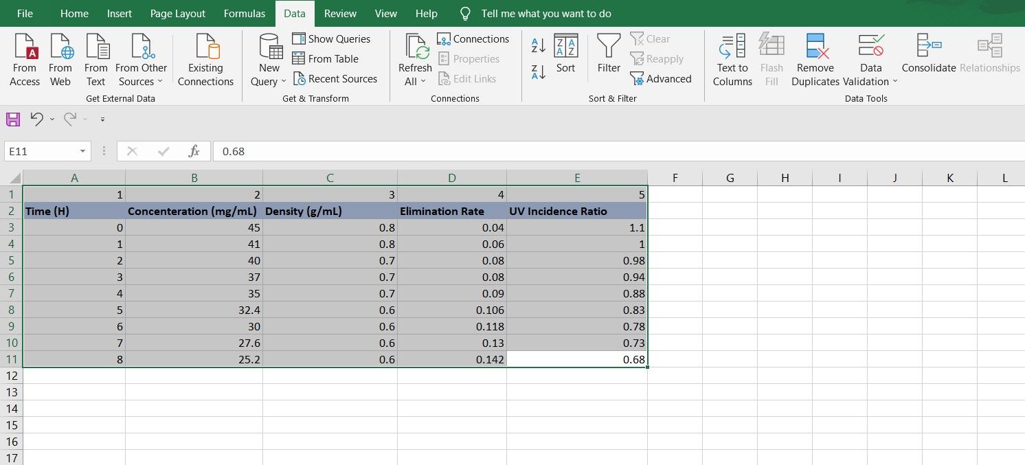
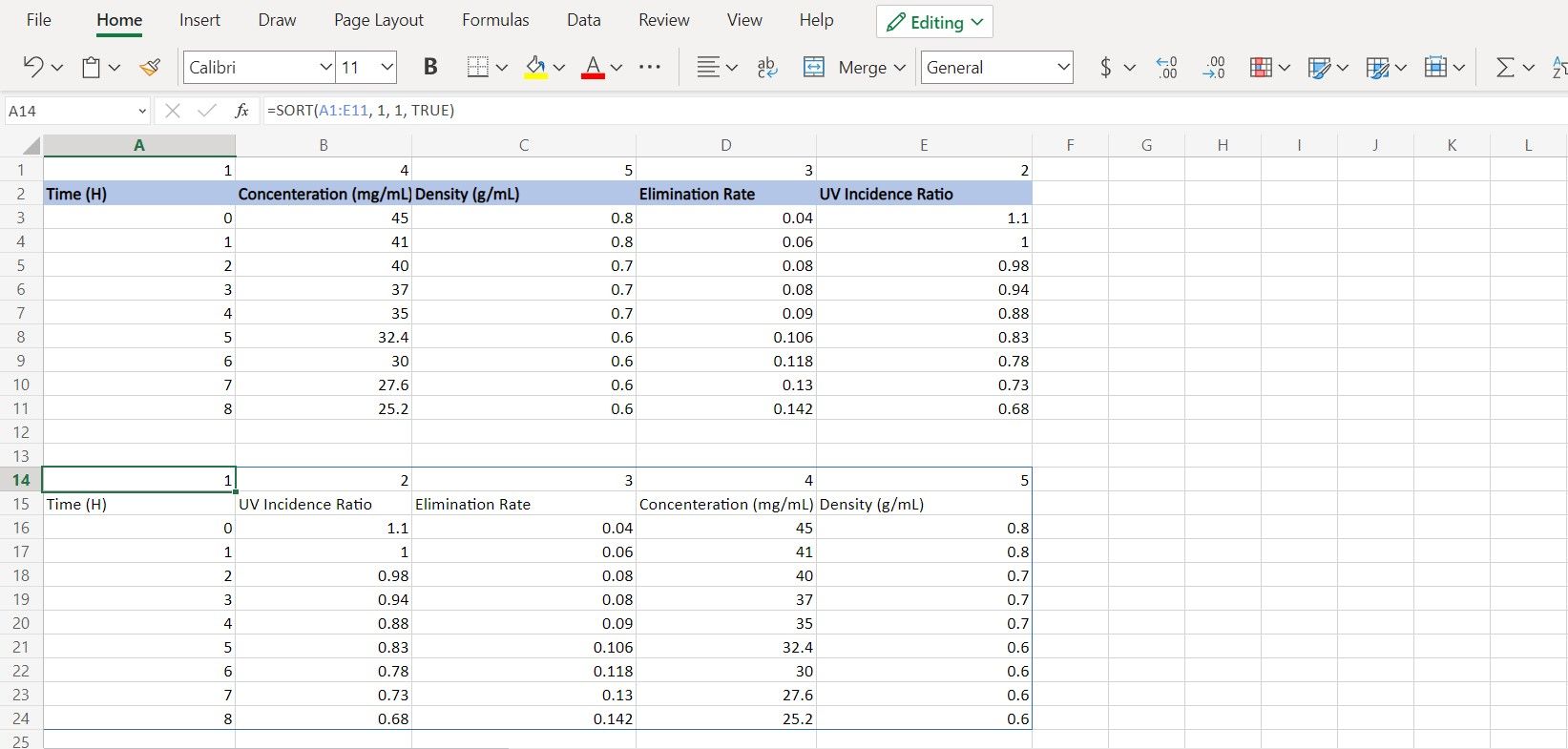
Right-click the first row and select Insert. This will insert a new row at the beginning of your table.
Inside the new row, insert the numeral order you’d like to arrange the columns by.
Select the cell where you want the new table.
In the formula bar, enter the formula below:
```
=SORT(array, 1, 1, TRUE)
```
- Insert your cell range (e.g. A1:E10) instead of an array. The sort_index is set to 1, which means the first row in the table will be used as the sort index. This is the row that we just created with the orders in it.
- The sort_order is set to 1, which means that the data order will be ascending. The column marked 1 will come before the column marked 2 and so forth.
- Finally, the by_column parameter is set to true because we want to sort the columns and not the rows.
Press Enter.

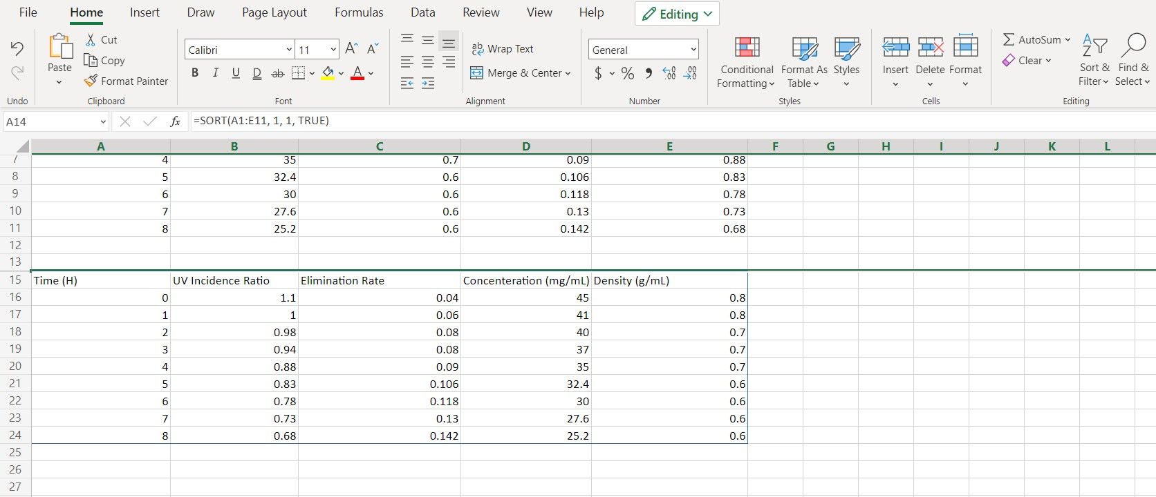
Now you have a sorted copy of your columns where you want them. Like the previous method, we have the unwanted top row here as well. This time you can’t just delete the row, because the row is part of an array formula, and you can’t change parts of an array formula. Nevertheless, you can still hide the row.

Right-click on the row number.
From the menu, select Hide Rows.

Put Your Excel Columns Where You Want

Data arrangement is a crucial element of your spreadsheet. By properly ordering and positioning the columns in a spreadsheet, you can improve its readability and make finding specific data in a spreadsheet easier.

In this article, we walked through four methods on how you can move the columns in Excel. With what you just learned, you know how to simply move columns by dragging or dropping them or to move multiple columns in one go using Data Sort or the SORT function in Excel.

Источник

See also

Things You Should Know

About This Article

Is this article up to date?

What to Know

Move Columns Using Your Mouse

Move a Column in Excel With Cut and Paste

Move Columns Using a Data Sort

Move Columns

Shift Key

Insert Cut Cells

Magic Move

How to Move Columns in Excel

In This Article

What to Know

Move Columns Using Your Mouse

Move a Column in Excel With Cut and Paste

Move Columns Using a Data Sort

How to swap columns by dragging and other ways to move columns in Excel

How to drag columns in Excel

Swap Excel columns by cutting and pasting

How to move one column in Excel

How to move several columns in Excel

Swap multiple columns by copying, pasting and deleting

Change the columns order in Excel using VBA

Re-arrange columns with Column Manager

1. Move Columns With Drag and Drop

2. Move Columns With Cut and Paste

3. Move Columns With Data Sort

4. Move Columns With the SORT Function

Put Your Excel Columns Where You Want