In an excel worksheet you can do this - Word и Excel - помощь в работе с программами

One of the FASTEST ways to Learn Excel is to learn some of the Excel TIPS and TRICKS, period and if you learn a single Excel tip a day you can learn 30 new things in a month.

But you must have a list that you can refer to every day instead of searching here and there. Well, I’m super PROUD to say that this is the most comprehensive list with all the basic and advanced tips that you can find on the INTERNET.

In this LIST, I have covered 300+ Excel TIPS and TRICKS which you can learn to Level Up your Excel Skills.

1. Add Serial Numbers

If you work with large data then it’s better to add a serial number column to it. For me, the best way to do this is to apply the table (Control + T) to the data and then add 1 in the above serial number, just like below.

To do this, you simply need to add 1 to the first cell of the column and then create a formula to add 1 to the above cell’s value. As you are using a table, whenever you create a new entry in the table, Excel will automatically drop down the formula and you will get the serial number.

2. Insert Current Date and Time

The best way to insert the current date and time is to use the NOW function which takes the date and time from the system and returns it.

excel tips tricks insert current date time

The only problem with this function is it’s volatile, and whenever you recalculate something it updates its value. And if you don’t want to do this, the best way is to convert it to hard value. You can also use the below VBA code.

Sub timestamp()
Dim ts As Date
With Selection
.Value = Now
.NumberFormat = "m/d/yyyy h:mm:ss AM/PM"
End With
End Sub

Or these methods to insert a timestamp in a cell.

3. Select Non-Continues Cells

Normally we all do it this way, hold the control key, and select cells one by one. But I have found that there is a far better way for this. All you have to do is, select the first cell and then press SHIFT + F8.

excel tips tricks select non adjacent cells without holding ctrl key

This gives you add or remove selection mode in which you can select cells just by selecting them.

4. Sort Buttons

If you deal with data that needs to sort frequently then it’s better to add a button to the quick access toolbar (if it’s not there already).

All you need to do is click on the down arrow on the quick access toolbar and then select “Sort Ascending” and “Sort Descending”. It adds both buttons to the QAT.

5. Move Data

I’m sure you think about copy-paste but you can also use drag-drop for this.

excel tips tricks move data with drag and drop

Simply select the range where you have data and then click on the border of the selection. By holding it move to the place where you need to put it.

6. Status Bar

The status bar is always there but we hardly use it to the full. If you right-click on it, you can see there are a lot of options you can add.

7. Clipboard

There is a problem with normal copy-paste that you can only use a single value at a time.

But here is the kicker: When you copy a value, it goes to the clipboard and if you open the clipboard you can paste all the values which you have copied. To open a clipboard, click on the go to Home Tab ➜ Editing and then click on the down arrow.

excel tips tricks click board open from home tab

It will open the clipboard on the left side, and you can paste values from there.

8. Bullet Points

The easiest way to insert bullet points in Excel is by using custom formatting and here are the steps for this:

Press Ctrl + 1 and you will get the “Format Cell” dialogue box.
Under the number tab, select custom.
In the input bar, enter the following formatting.
1. ● General;● General;● General;● General
In the end, click OK.

excel tips tricks custom formatting for bullet points

Now, whenever you enter a value in the cell Excel will add a bullet before that.

9. Worksheet Copy

To create a copy of a worksheet in the same workbook drag and drop in the best way.

You just need to click and hold the mouse on the sheet’s name tab and then drag and drop it, to the left or right, where you want to create a copy.

10. Undo-Redo

Just like sort buttons you can also add undo and redo buttons to the QAT. The best part about those buttons is you can use them to undo a particular activity without pressing the shortcut key again and again.

11. AutoFormat

If you deal with financial data, then auto format can be one of your best tools. It simply applies the format to small as well as large data sets (especially when data is in tabular form).

First of all, you need to add it to the quick access toolbar (here are the steps).
After that, whenever you need to apply the format, just select the data where you want to apply it and click on the AUTO FORMAT button from the quick access toolbar.
It will show you a window to select the formatting type and after selecting that click OK.

The AUTOFORMAT is a combination of six different formattings and you have the option to disable any of them while applying it.

12. Format Painter

The simple idea with the format painter is to copy and paste formatting from one section to another. Let’s say you have specific formatting (Font Style and Color, Background Color to a Cell, Bold, Border, etc.) in the range B2:D7, and with format painter, you can copy that formatting to range B9: D14 with a click.

First of all, select the range B2:D7.
After that, go to the Home Tab ➜ Clipboard and then click on “Format Painter”.
Now, select cell C1 and it will automatically apply the formatting on B9: D14.

The format painter is fast and makes it easy to apply to format from one section to another.

Related: Format Painter Shortcut

13. Cell Message

Let’s say you need to add a specific message to a cell, like “Don’t delete the value”, “enter your name” or something like that.

In this case, you can add a cell message for that particular cell. When the user will select that cell, it will show the message you have specified. Here are the steps to do this:

excel tips tricks create cell message display

First, select the cell to which you want to add a message.
After that, go to the Data Tab ➜ Data Tools ➜ Data Validation ➜ Data Validation.
In the data validation window, go to the Input Message tab.
Enter the title, and message, and make sure to tick mark “Show input message when the cell is selected”.
In the end, click OK.

Once the message is shown you can drag and drop it to change its position.

14. Strikethrough

Unlike Word, in Excel, there is no option on the ribbon to apply strikethrough. But I have figured out that there are 5 ways to do it and the easiest of all of them is a keyboard shortcut.

All you need to do is select the cell where you want to apply the strikethrough and use the below keyboard shortcut.

Ctrl + 5

And if you are using MAC then:

⌘ + ⇧ + X

Quick Note: You can use the same shortcut keys if you need to do this for partial text.

15. Add Barcode

It is one of those secret tips that most Excel users are unaware of. To create a bar-code in Excel all you need to do is install this bar-code font from ID-AUTOMATIC.

Once you install this font, you will have to type the number in a cell for which you want to create a bar code and then apply the font style.

15 excel tips tricks install barcode font

learn more about this tip

16. Month Name

Alright, let’s say you have a date in a cell, and you want that date to show as a month or a year. For this, you can apply custom formatting.

16 excel tips tricks show date as month year

First, select the cell with a date and open formatting options (use Ctrl + 1).
Select the “Custom” option and add “MMM” or “MMMMMM” for the month or “YYYY” for the year format.
In the end, click OK.

Custom formatting just changes the formatting of the cell from date to year/month, but the value remains the same.

17. Highlight Blank Cells

When you work with large data sheets it’s hard to identify the blank cells. So, the best way is to highlight them by applying a cell color.

First, select all the data from the worksheet using the shortcut key Ctrl + A.

excel tips and tricks to highlight blank cells select data

After that, go to Home Tab ➜ Editing ➜ Find & Select ➜ Go to Special.

excel tips and tricks to highlight blank cells click goto special

From Go to Special dialog box, select Blank and click OK.

excel tips and tricks to highlight blank cells click blank option

At this point, you have all the blank cells selected and now apply a cell color using font settings.

excel tips and tricks to highlight blank cells apply color

…but you can also use conditional formatting for this

18. Font Color with Custom Formatting

In Excel, we can apply custom formatting and in custom formatting, there is an option to use font colors (limited but useful).

For example, if you want to use the Green color for positive numbers and the red color for negative numbers then you need to use the custom format.

[Green]#,###;[Red]-#,###;0;

excel tips and tricks to red green negative positive numbers add custom formatting

First, select the cells where you want to apply this format.
After that open the format option using the keyboard shortcut Ctrl + 1 and go to the “Custom” category and the custom format in the input dialogue box.
In the end, click OK.

19. Theme Color

We all have some favorite fonts and colors which we use in Excel. Let’s say you received a file from your colleague and now you want to change the font and colors for the worksheet from that file. The point is, you need to do this one by one for each worksheet and that takes time.

But if you create a custom theme with your favorite colors and fonts then you can change the style of the worksheet with a single click. For this, all you have to do is apply your favorite designs to the tables, colors to the shapes and charts, and font style, and then save it as a custom theme.

Go to the Page Layout Tab ➜ Themes ➜ Save Current Theme. It opens a “Save As” dialogue box, names your theme, and saves it.
And now, every time you need just one click to change any worksheet style to your custom style.

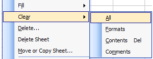
20. Clear Formatting

This is a simple keyboard shortcut that you can use to clear formatting from a cell or range of cells.

Alt ➜ H ➜ E ➜ F

Or, otherwise, you can also use the clear formatting option from the Home Tab (Home Tab ➜ Editing ➜ Clear ➜ Formats).

21. Sentence Case

In Excel, we have three different functions (LOWER, UPPER, and PROPER) to convert text into different cases. But there is no option to convert a text into a sentence case. Here is the formula which you can use:

=UPPER(LEFT(A1,1))&LOWER(RIGHT(A1,LEN(A1)-1))

excel tips and tricks to convert to sentence case

This formula converts the first letter of a sentence into capital and the rest all in small (learn how this formula works).

22. Random Numbers

In Excel, there are two specific functions that you can use to generate random numbers. First is RAND which generates random numbers between 0 and 1.

And second is RANDBETWEEN which generates random numbers within the range of two specific numbers.

ALERT: These functions are volatile so whenever you re-calculate your worksheet or hit enter, they update their values so make sure to use them with caution. You can also use RANDBETWEEN to generate random letters and random dates.

23. Count Words

In Excel, there is no specific function to count words. You can count characters with LEN but not words. But, you can use the following formula which can help you to count words from a cell.

=LEN(A1)-LEN(SUBSTITUTE(A1,” “,”))+1

This formula counts the number of spaces from a cell and adds 1 to it after that which equals the total number of words in a cell.

24. Calculate the Age

The best way to calculate a person’s age is by using the DATEDIF. This mysterious function is specifically made to get the difference between a date range.

And the formula will be:

=”Your age is “& DATEDIF(Date-of-Birth,Today(),”y”) &” Year(s), “& DATEDIF(Date-of-Birth,TODAY(),”ym”)& ” MONTH(s) & “& DATEDIF(Date-of-Birth,TODAY(),”md”)& ” Day(s).”

25. Calculate the Ratio

I have figured out that there are four different ways to calculate the ratio in Excel but using a simple divide method is the easiest one. All you need to do is divide the larger number into the smaller ones and concatenate it with a colon and one and here’s the formula you need to use:

=Larger-Number/Smaller-Number&”:”&”1″

excel tips tricks to use simple divide to calculate ratio in excel

This formula divides the larger number by the smaller one so that you can take the smaller number as a base (1).

26. Root of Number

To calculate the square root, cube root, or any root of a number the best way is to use the exponent formula. In the exponent formula, you can specify the Nth number for which you want to calculate the root.

=number^(1/n)

For example, if you want to calculate a square root of 625 then the formula will be:

=625^(1/2)

28. Month’s Last Date

To simply get the last date of a month you can use the following dynamic formula.

=DATE(YEAR(TODAY()),MONTH(TODAY())+1,0)

excel tips and tricks to end of the month date

29. Reverse VLOOKUP

As we all know there is no way to look up to left for a value using VLOOKUP. But if you switch to INDEX MATCH you can look up in any direction.

30. SUMPRODUCT IF

You can use the below formula to create a conditional SUMPRODUCT and product values using a condition.

=SUMPRODUCT(–(C7:C19=C2),E7:E19,F7:F19)

31. Smooth Line

If you love to use a line chart, then you are awesome but it would be more awesome if you use a smooth line in the chart. This will give a smart look to your chart.

Select the data line in your chart and right-click on it.
Select “Format Data Series”.
Go to Fill & Line ➜ Line ➜ Tick mark “Smoothed Line”.

excel tips tricks charting tips smooth line chart

33. Hide Axis Labels

This charting tip is simple but still quite functional. If you don’t want to show axis label values in your chart you can delete them. But the better way is to hide them instead of deleting them. Here are the steps:

Select the Horizontal/Vertical axis in the chart.
Go to “Format Axis” Labels.
In the label position, select “None”.

And again, if you want to show it then just select “Next to axis”.

34. Display Units

If you are dealing with large numbers in your chart, you can change the units for axis values.

excel tips tricks to hide axis label before after

Select the chart axis of your chart and open the format “Format Axis” options.
In axis options, go to “Display Units” where you can select a unit for your axis values.

35. Round Corner

I often use Excel charts with rounded corners and if you like to use round corners too, here are the simple steps.

Select your chart and open formatting options.
Go to Fill and Line ➜ Borders.
In borders sections, tick mark rounded corners.

36. Hide Gap

Let’s say you have a chart with monthly sales in which June has no amount and the cell is empty. You can use the following options for that empty cell.

excel tips tricks to fill gap for empty values

Show the gap for the empty cell.
Use zero.
Connect data points with the line.

Here are the steps to use these options.

Right, click on your chart & select “Select Data”.
In the select data window, click on “Hidden and Empty Cell”.
Select your desired option from “Show Empty Cell as”.

excel charting tips to remove chart gap select connect data

Make sure to use “Connect data points with the line” (recommended).

38. Chart Template

Let’s say you have a favorite chart formatting you want to apply every time you create a new chart. You can create a chart template to use anytime in the future and the steps are as follow.

Once you have done with your favorite formatting, right-click on it & select “Save As Template”.

excel charting tips save as template right click

Using the save as dialog box, save it in the template folder.
To insert a new one with your favorite template, select it from templates in the insert chart dialog.

excel charting tips save as template apply chart

39. Default Chart

You can use a shortcut key to insert a chart, but the problem is, it will only insert the default chart, and in Excel, the default chart type is “Column Chart”. So if your favorite chart is a line chart, then the shortcut is useless for you. But let’s conquer this problem. Here are the steps to fix this:

Go to Insert Tab ➜ Charts.
Click on the arrow at the bottom right corner.
Then in your insert chart window, go to “All Charts” and then select the chart category.
Right, click on the chart style you want to make your default Select “Set as Default Chart”.
Click OK.

excel charting tips change default chart

40. Hidden Cells

When you hide a cell from the data range of a chart, it will hide that data point from the chart as well. To fix this, just follow these steps.

Select your chart and right-click on it.
Go to ➜ Select Data ➜ Hidden and empty cells.
From the pop-up window, tick the mark “Show data in hidden rows and columns”.

41. Print Titles

Let’s say you have headings on your table, and you want to print those headings on every page you print. In this case, you can fix “Print Titles” to print those headings on each page.

Go to “Page Layout Tab” ➜ Page Set Up ➜ Click on Print Titles.
Now in the page setup window go to the sheet tab and specify the following things.

Print Area: Select the entire data which you want to print.
Rows to repeat at the top: Heading row(s) which you want to repeat on every page.
Columns to repeat at the left: Column(s) which you want to repeat at the left side of every page (if any).

42. Page Order

Specifying the page order is quite useful when you want to print large data.

Go to File Tab ➜ Print ➜ Print Setup ➜ Sheets Tab.
Now here, you have two options:
- The First Option: To print your pages using a vertical order.
- The Second Option: To print your pages using a horizontal order.

excel tips tricks set printing direction

If you add comments to your reports then you can print them as well. At the end of all printed pages, you can get a list of all the comments.

Go to File Tab ➜ Print ➜ Print Setup ➜ Sheets Tab.
In the print section, select “At the end of the sheet” using the comment dropdown.
Click OK.

44. Scale to Fit

Sometimes we struggle to print entire data on a single page. In this situation, you can use the “Scale to Fit” option to adjust the entire data into a single page.

Go to File Tab ➜ Print ➜ Print Setup ➜ Page Tab.
Next, you need to adjust two options:
1. Adjust % of normal size.
2. Specify the number of pages in which you want to adjust your entire data using width and length.

Instead of using the page number in the header and footer, you can also use a custom header and footer.

Go to File Tab ➜ Print ➜ Print Setup ➜ Header/Footer.
Click on the custom header or footer button.

Here you can select the alignment of the header/footer.

And the following options can be used:
1. Page Number
2. Page Number with total pages.
3. Date
4. Time
5. File Path
6. File Name
7. Sheet Name
8. Image

46. Center on Page

Imagine you have less data to print on a page. In this case, you can align it at the center of the page while printing.

Go to File Tab ➜ Print ➜ Print Setup ➜ Margins.
In “Center on Page” you have two options to select.
- Horizontally: Aligns data to the center of the page.
- Vertically: Aligns data to the middle of the page.

Before printing a page make sure to see the changes in the print preview.

47. Print Area

The simple way to print a range is to select that range and use the option “print selection”. But what if you need to print that range frequently, in that case, you can specify the printing area and print it without selecting it every time.

Go to the Page Layout Tab, click on the Print Area drop-down, and after that, click on the Set Print Area option.

48. Custom Margin

Go to File Tab ➜ Print.
Once you click on print, you’ll get an instant print preview.
Now from the bottom right side of the window, click on the “Show Margins” button.

It will show all the margins applied and you can change them just by dragging and dropping.

49. Error Values

You can replace all the error values while printing with a specific value (three other values to use as a replacement).

Go to File Tab ➜ Print ➜ Print Setup ➜ Sheet.
Select the replacement value from the “Cell error as” dropdown.
You have three options to use as a replacement.
1. Blank
2. Double minus sign.
3. “#N/A” error for all the errors.

After selecting the replacement value, click OK.

I believe using a “Double minus sign” is the best way to present errors in a report while printing it on a page.

Related: Ignore All the Errors

50. Custom Start Page Number

If you want to start the page number from a custom number let’s say 5. You can specify that number and the rest of the pages will follow that sequence.

Go to File Tab ➜ Print ➜ Print Setup ➜ Page.
In the input box “First page Number”, enter the number from where you want to start the page number.

In the end, click OK.

This option will only work if you have applied the header/footer in your worksheet.

51. Tracking Important Cells

Sometimes we need to track some important cells in a workbook and for this, the best way is to use the watch window. In the watch window, you add those important cells and then get some specific information about them in one place (without navigating to each cell).

First, go to Formula Tab ➜ Formula Auditing ➜ Watch Window.

Now in the “Watch Window” dialog box, click on “Add Watch”.

After that select the cell or range of cells that you want to add and click OK.

Once you hit OK, you’ll get some specific information about the cell(s) in the watch window.

52. Flash Fill

Flash fill is one of my favorite options to use in Excel. It’s like a copycat, perform the task which you have performed. Let me give you an example.

Here are the steps to use it: You have dates in the range A1: A10 and now, you want to get the month from the dates in the B column.

All you need to do is to type the month of the first date in cell B1 and then come down to cell B2 and press the shortcut key CTRL + E. Once you do this it will extract the month from the rest of the dates, just like below.

53. Combine Worksheets

I’m sure somewhere in the past you have received a file from your colleague where you have 12 different worksheets for 12 months of data. In this case, the best solution is to combine all of those worksheets using the “Consolidate” option, and here are the steps for this.

First, add a new worksheet and then go to Data Tab ➜ Data Tools ➜ Consolidate.

Now in the “Consolidate” window, click on the upper arrow to add the range from the first worksheet and then click on the “Add” button.
Next, you need to add references from all the worksheets using the above step.

In the end, click OK.

54. Protect a Workbook

Adding a password to a workbook is quite simple, here are the steps.

While saving a file when you open a “Save As” dialog box go to Tools General Options.

Add a password to “Password to Open” and click OK.

Re-enter the password and click OK again.
In the end, save the file.

Now, whenever you re-open this file it will ask you to enter the password to open it.

55. Live Image

In Excel, using a live image of a table can help you resize it according to space, and to create a live image there are two different ways in which you can use it.

One is camera tools and the second is the paste special option. Here are the steps to use the camera tool and for paste special use the below steps.

Select the range you want to paste as an image and copy it.
Go to the cell and right-click, where you want to paste it.
Go to Paste Special ➜ Other Paste ➜ Options Linked Picture.

56. Userform

A few of the Excel users know that there is a default data entry form is there which we can use. And the best part is there is no need to write a single line of code for this.

Here’s how to use it:

First of all, make sure you have a table with headings where you want to enter the data.
After that select any of the cells from that table and use the shortcut key Alt + D + O + O to open the user form.

57. Custom Tab

We all have some favorite options or some options which we use frequently. To access all those options in one place you create a tab and add them to it.

First, go to File Tab ➜ Options ➜ Customize Ribbon.
Now click on “New Tab” (this will add a new tab).
After that right-click on it and name it and then name the group.
Finally, we need to add options to the tab and for this go to “Choose Commands From” and add them to the tab one by one.
In the end, click OK.

59. Text to Speech

This is an option where you can make Excel speak the text you have entered into a cell or a range of cells.

60. Named Range

To create a named range the easiest method is to select the range and create it using the “Create from Selection” option. Here are the steps to do this:

Select the column/row for which you want to create a named range.
Right-click and click on “Define name…”.

Select the option to add the name for the named range and click OK.

That’s it.

61. Trim

TRIM can help you to remove extra spaces from a text string. Just refer to the cell from where you want to remove the spaces and it will return the trimmed value in the result.

62. Remove Duplicates

One of the most common things we face while working with large data is “Duplicate Values”. In Excel, removing these duplicate values is quite simple. Here’s how to do this.

First, select any of the cells from the data or select the entire data.
After that, go to Data ➜ Data Tools ➜ Remove Duplicates.
At this point, you have the “Remove Duplicates” window, and from this window, select/de-select the columns which you want to consider/not consider while removing duplicate values.
In the end, click OK.

Once you click OK, Excel will remove all the rows from the selected data where values are duplicates and show a message with the number of values removed and unique values left.

64. Remove Specific Character

In the range, A1: A5 and you want to concatenate all of them in a single cell. Here’s how to do this with fill justify.

All you need to do is select that column and open the find and replace dialog box.
After that click on the “Replace” tab.
Now here, in “Find What” enter the character you want to replace and make sure to leave “Replace with” blank.
Now click on “Replace All”.

The moment you click on “Replace All” Excel will remove that particular character from the entire column.

Related: Remove First Character from a Cell in Excel

65. Combine Text

So, you have text in multiple cells, and you want to combine all the text into one cell. No, this time not with fill justify. We are doing it with TEXT JOIN. If you use Office 365, there is a new function TEXTJOIN which is a game-changer when it comes to the concatenation of text.

Here’s the syntax:

TEXTJOIN(delimiter, ignore_empty, text1, [text2], …)

All you need to do is to add a delimiter (if any), and TRUE if you want to ignore empty cells, and in the end, refer to the range.

66. Unpivot Data

Look at the below table, you can use it as a report but you can’t use it further as raw data. No, you can’t. But if you convert this table to something like the one below you can use it easily anywhere.

But if you convert this table into something like the one below you can use it easily anywhere. So how to do this?

here are the simple steps you need to follow.

67. Delete Error Cells

Mostly while working with large data it is obvious to have error values but it’s not good to keep them. The easiest way to deal with these error values is to select them and delete them and these are the simple steps.

First of all, go to Home Tab ➜ Editing ➜ Find & Replace ➜ Go To Special.
In the Go To dialog box, select formula, and tick mark errors.

In the end, click OK.

Once you click OK it will select all the errors and then you can simply delete all by using the “Delete” button.

68. Arrange Columns

Let’s say you want to arrange columns from the data using custom order. The normal way is to cut and paste them one by one.

But we also have an out-of-the-box way. In Excel, you can sort columns just like you sort rows and by using the same methods you can arrange them in a custom order.

⇢ Complete Tip

69. Convert to Date

Sometimes you have dates that are stored as text and you can use them in a calculation and further analysis. To simply convert them back to valid dates you can use the DATEVALUE function.

Other ways to convert text to date

71. Format Painter

Before I started to use format painter for applying cell formatting, I was using paste special with the shortcut key.

Select the cell or a range from where you want to copy cell formatting.
Go to ➜ the Home Tab ➜ Clipboard.
Make double-click on the “Format Painter” button.
As soon as you do this, your cursor will convert into a paintbrush.
You can apply that formatting anywhere in your worksheet, in another worksheet, or, even in another workbook.

72. Rename a Worksheet

I always found it quicker than using a shortcut key to change the name of a worksheet. All you have to do is just double-click on the sheet tab and enter a new name.

Let me tell you why this method is faster than using a shortcut. Suppose if want to rename more than one worksheet using a shortcut key.

Before you change the name of a worksheet, you need to activate it. But if you use the mouse it will automatically activate that worksheet and edit the name with only two clicks.

73. Fill Handle

I am sure shortcut addicts always use a shortcut key to drag formulas and values in downward cells. But using a fill handle is more impressive than using a shortcut key.

Select the cell in which you have a formula or a value that you want to drag.
Make a double click on the small square box at the right bottom of the cell selection border.

This method only works if you have values in the corresponding column and it works only in the vertical direction.

74. Hide Ribbon

If you want to work in a distraction-free mode, you can do this by collapsing your Excel ribbon.

Just make double-click on the active tab in your ribbon and it will collapse the ribbon. And if you want to expand it back just double-click on it again.

75. Edit a Shape

You often use shapes in our worksheets to present some messages and you have to insert some text into those shapes. Besides the typical method, you can use a double click to edit a shape and insert the text into it.

You can also use this method to edit and enter text in a text box or into a chart title.

76. Column Width

Whenever you have to adjust the column width you can double-click on the right edge of the column header. It auto-sets the column width according to the column data.

The same method can be used to auto-adjust row width.

77. Go to the Last Cell

This trick can be useful if you are working with a large dataset. By using a double click, you can go to the last cell in the range which has data.

You have to click on the right edge of the active cell to go to the right side and on the left edge if you want to go to the left side.

78. Chart Formatting

If you use Control + 1 to open formatting options to format a chart, then I bet you’ll love this trick. All you have to do is just make double-click on the border of the graph to open the formatting option.

79. Pivot Table Double Click

Let’s say someone sent you a pivot table without the source data. As you already know Excel stores data in a pivot cache before creating a pivot table.

You can extract data from a pivot table by double-clicking on data values. As soon as you do this Excel will insert a new worksheet with the data which has been used in the pivot table.

There is a right-click drop-down menu in Excel that few users know about. To use this menu all you need to do is select a cell or a range of the cell and then right-click and while holding it, drop the selection to somewhere else.

81. Default File Saving Location

Normally while working on Excel I create more than 15 Excel files every day. And, if I save each of these files to my desktop it looks nasty. To solve this problem, I have changed my default folder for saving a workbook, and here’s you can do this.

First, go to the File tab and open Excel options.
In Excel options, go to the “Save” category.
Now, there is an input bar where you can change the default local file location.
From this input bar, change the location address and in the end, click OK.

From now onward, when you open the “Save As” dialog box Excel will show you the location you have specified.

82. Disable Start Screen

I’m sure just like me you hate when you open Microsoft Excel (or any other Office app) and you see the start pop-up screen. It takes time depending on your system’s speed and the add-ins you have installed. Here are the steps to disable the start-up screen in Microsoft Office.

First, go to the File tab and open Excel options.
In Excel options, go to the “General” category.
From the option, drill down to the “Start-Up” options and un-tick the “Show the Start screen when this application starts”.
In the end, click OK.

From now onward, whenever you start Excel it will directly open the workbook without showing the start-up screen.

83. Developer Tab

Before you start writing VBA codes the first thing you need to do is to enable the “Developer Tab”. When you first install Microsoft Excel, a developer wouldn’t be there. So, you need to enable it from the settings.

First, go to the File tab and click on the “Customize Ribbon” category.
Now from the tab list, tick marks the developer tab and click OK.

Now when you come back to your Excel window, you’ll have a developer tab on the ribbon.

84. Enable Macros

When you open a macro-enabled file, you need to enable macro options to run VBA codes. Follow these simple steps:

First, go to the File tab and click on the “Trust Center” category.
From here click on “Trust Center Settings”.
Now in “Trust Center Settings”, click on macro settings.
After that, click on “Enable all macros with Notifications”.
In the end, click OK.

85. AutoCorrect Option

If you do a lot of data entry in Excel, then this option can be a game-changer for you. With the auto-correct option, you can tell Excel to change a text string into another when you type it.

Let me tell you an example:

My name is “Puneet” but sometimes people write it like “Punit” but the correct spelling is the first one. So, what I can do is, use autocorrect and tell Excel to change “Punit” into “Puneet”. Follow these simple steps:

First, go to the File tab and go to options and click on the “Proofing” category.
After that, click on “AutoCorrect Option” and this will open the auto-correct window.
Here in this window, you have two input bars to specify the text to replace and text to replace with.
Enter both values and then click OK.

86. Custom List

Just think like this, you have a list of 10 products that you sell. Whenever you need to insert those product names you can insert them using a custom list. Let me tell you how to do this:

First, go to the File tab and go to options and click on the “Advanced” category.
Now, drill down and go to the “General” section and click on “Edit Custom List…”.
Now in this window, you can enter the list, or you can also import it from a range of cells.
In the end, click OK.

Now, to enter the custom list you have just created, enter the first entry of the list in the cell and then drill down that cell using the fill handle.

87. Apply Table

If you use pivot tables a lot then it’s important to apply the table to the raw data. With a table, there is no need to update the pivot table’s data source, and it drag-down formulas automatically when you add a new entry.

To apply the table to the data just use Ctrl + T keyboard shortcut key and click OK.

88. Gridline Color

If you are not happy with the default color of cell gridlines then you can simply change it with a few clicks and follow these simple steps for this:

First, go to the File tab and click on the “Advanced” category.
Now, go to the “Display options for this workbook” section and select the color you want to apply.

In the end, click OK.

Related – Print Gridlines

89. Pin to Taskbar

This is one of my favorite one-time sets up to save time in the long run. The thing is instead of going to the start menu to open Microsoft Excel, the best way is to point it to the taskbar.

This way you can open it by clicking on the icon from the taskbar.

90. Macro to QAT

If you have a macro code that you need to use frequently. Well, the easiest way to run a macro code is to add it to the Quick Access Toolbar.

First, go to the File tab and click on the “Quick Access Toolbar” category.
After that, from “Choose Command from”, select Macros.
Now select the macro (you want to add to QAT) and click on add.
From here click on “Modify” and select an icon for the macro button.
In the end, click OK.

Now you have a button on QAT that you can use to run the macro code you have just specified.

Related – How to Record a Macro in Excel

91. Select Formula Cells

Let’s say you want to convert all the formulas into values and the cells where you have formulas are non-adjacent. So instead of selecting each cell one by one, you can select all the cells where you have a formula. Here are the steps:

First, go to Home Tab ➜ Editing ➜ Find & Select ➜ Go To Special.
In the “Go To Special” dialog box, select formulas and click OK.

92. Multiply using Paste Special

To do some one-time calculations you can use the paste special option and save yourself from writing formulas.

93. Highlight Duplicate Values

Well, you can use a VBA code to highlight values but the easiest way is to use conditional formatting. Here are the steps you need to follow:

First of all, select the range where you want to highlight the duplicate values.
After that, go to Home Tab ➜ Styles ➜ Highlight Cells Rule ➜ Duplicate Values.
Now from the dialog box, select the color to use and click OK.

Once you click OK, all the duplicate values will get highlighted.

94. Quick Analysis Tool

If you ever noticed that when you select a range of cells in Excel, a small icon at the bottom of the selection appears? This icon is called the “Quick Analysis Tool”.

When you click on this icon you can see some of the options which are there on the ribbon which you can directly use from here to save time.

95. RUN Command

Yes, you can also open your Excel application using the RUN command.

For this, all you have to do is open RUN (Window Key + R) and then type “excel” into it.
In the end, hit enter.

96. Open Specific File

I’m sure like me you also have a few or maybe one of those kinds of workbooks that you open every day when you start working on Excel. There is an option in Excel which you can use to open a specific file(s) whenever you start Excel in your system. Here are the steps.

Go to File ➜ Options ➜ Advanced ➜ General.
In general, enter the location (yes, you have to type) of the folder where you have those file(s) in “At startup open all the files in”.

97. Open Excel Automatically

Whenever I “Turn ON” my laptop the first thing I do is open Excel and I’m sure you do the same thing. Well, I’ve got a better idea here, you can add Excel to your system’s startup folder.

First, open “File Explorer” by using the Windows key + E.
Now, enter the below address into the address bar to open the folder (change the username with your actual username).
- C:UsersUserAppDataRoamingMicrosoftWindowsStart MenuProgramsStartup
After that, open the Start Screen, right-click on the Excel App, and click Open file location.
From the location (Excel App Folder), copy the Excel App icon and paste it into the “Startup” folder.

Now whenever you open your system, Excel will automatically start.

98. Smart Look Up

In Excel, there is an option called “Smart Lookup” and with this option, you can look up a text on the internet. All you have to do is, select a cell or a text from a cell, and go to Review ➜ Insights ➜ Smart Lookup.

excel tips tricks smart lookup press button

Once you click on it, it opens a side pane where you’ll have information about that particular text which you have selected. The idea behind this option is to get information by seeing definitions, and images for the topic (text) from different online sources.

99. Screen Clipping

Sometimes you need to add screenshots to your spreadsheet. And for this, Excel has an option that can capture the screen instantly, and then you can paste it into the worksheet. For this go to ➜ Insert ➜ Illustrations ➜ Screen Clipping.

Related – Excel Camera

100. Locate a Keyboard Shortcut

If you use Excel 2007 to Excel 2016, then you can locate a keyboard shortcut by pressing the ALT key. Once you press it, it shows the keys for the options which are there on the ribbon, just like below.

Let’s say, you want to press the “Wrap Text” button, and the key will be ALT H W. In the same way you can reach all the options using the shortcut keys.

Related – Insert Row

101-300

Add and Delete a Worksheet in Excel
Add and Remove Hyperlinks in Excel
Add Watermark in Excel
Apply Accounting Number Format in Excel
Delete Hidden Rows in Excel
Deselect Cells in Excel
Draw a Line in Excel
Formula Bar in Excel
Add a Button in Excel
Add a Column in Excel
Apply Comma Style in Excel
Group Worksheets in the Excel
Make Negative Numbers Red in Excel
Merge – Unmerge Cells in Excel
Show Ruler in Excel
Spell Check in Excel
Fill Handle in Excel
View Two Sheets Side by Side in Excel
Increase and Decrease Indent in Excel
Insert an Arrow in a Cell in Excel
Remove Pagebreak in Excel
Rotate Text in Excel (Text Orientation)
Row Vs Column in Excel (Difference)
Delete Blank Rows in Excel
Sort By Date, Date, and Time & Reverse Date Sort in Excel
Find and Replace in Excel
Make a Paragraph in a Cell in Excel
Cell Style (Title, Calculation, Total, Headings…) in Excel
Hide and Unhide a Workbook in Excel
Change Date Format in Excel
Center a Worksheet Horizontally and Vertically in Excel
Make a Copy of the Excel Workbook (File)
Write (Type) Vertically in Excel
Add or Remove Grand Total in a Pivot Table in Excel
Add Running Total in a Pivot Table in Excel
Add Calculated Field and Item (Formulas in a Pivot Table)
Count Unique Values in a Pivot Table in Excel
Delete a Pivot Table in Excel
Filter a Pivot Table in Excel
Add Ranks in Pivot Table in Excel
Apply Conditional Formatting to a Pivot Table
Pivot Table using Multiple Files in Excel
Group Dates in a Pivot Table
Link a Single Slicer with Multiple Pivot Tables
Move a Pivot Table
Pivot Table Formatting
Pivot Table Keyboard Shortcuts
Pivot Table Timeline in Excel
Refresh a Pivot Table
Refresh All Pivot Tables at Once in Excel
Sort a Pivot Table in Excel
Apply Print Titles in Excel (Set Row 1 to Print on Every Page)
Apply Multiple Filters to Columns
Create a Data Validation with Date Range
Create a Yes – No Drop Down in Excel
Merge Cells in Excel without Losing Data in Excel
Remove Drop Down List (Data validation) in Excel
Formulas in Conditional Formatting
Print a Graph Paper in Excel (Square Grid Template)
Recover Unsaved Excel Files When Excel Crashed
Save Excel File (Workbook) as CSV (XLSX TO CSV)
Create a Pivot Table from Multiple Worksheets
Create Pivot Chart in Excel
Activate a Sheet using VBA
Create WAFFLE CHART in Excel
Excel Funnel Chart (Template + Steps to Create)
Excel Gantt Chart Template
Add a Horizontal Line in a Chart in Excel
Add a Vertical Line in a Chart in Excel
Create a Bullet Chart in Excel
Create a Dynamic Chart Range in Excel
Create a HEAT MAP in Excel (Simple Steps) + Template
Create a Milestone Chart in Excel
Create a Population Pyramid Chart in Excel
Create a Step Chart in Excel
Create a Tornado Chart in Excel
Create Interactive Charts in Excel
Insert a People Graph in Excel
Top 10 ADVANCED Excel Charts and Graphs (Free Templates Download)
Add Secondary Axis in Excel Charts
Create a HISTOGRAM in Excel – Step by Step
SPEEDOMETER Chart in Excel
Thermometer Chart in Excel
Merge [Combine] Multiple Excel FILES into ONE WORKBOOK
Perform VLOOKUP in Power Query in Excel
Calculate the Coefficient of Variation (CV) in Excel
Does Not Equal Operator in Excel
MAX IF in Excel
Round a Number to Nearest 1000, 100, and 10 in Excel
Round to Nearest .5, 5. 50 (Down-Up) in Excel
Square a Number in Excel
#DIV/0
#SPILL!
#Value
3D Reference in Excel
Wildcard Characters in Excel
Hide Formula in Excel
R1C1 Reference Style in Excel
VLOOKUP with Multiple Criteria in Excel
Wildcards with VLOOKUP in Excel
Average TOP 5 Values in Excel
Calculate Compound Interest in Excel
Calculate Cube Root in Excel
Calculate Percentage Variance (Difference) in Excel
Calculate Simple Interest in Excel
Calculate the Weighted Average in Excel

Absolute Reference (Excel Shortcut)
Add Column (Excel Shortcut)
Add Indent (Excel Shortcut)
Add New Sheet (Excel Shortcut)
Align Center (Excel Shortcut)
Apply Border (Excel Shortcut)
Apply and Remove Filter (Excel Shortcut)
Auto Fit (Excel Shortcut)
AutoSum (Excel Shortcut)
Check Mark (Excel Shortcut)
Clear Contents (Excel Shortcut)
Close (Excel Shortcut)
Currency Format (Excel Shortcut)
Delete Cell (Excel Shortcut)
Delete Row(s) (Excel Shortcut)
Delete Sheet (Excel Shortcut)
Edit Cell (Excel Shortcut)
Fill Color (Excel Shortcut)
Freeze Pane (Excel Shortcut)
Full Screen (Excel Shortcut)
Group (Excel Shortcut)
Hyperlink (Excel Shortcut)
Insert Cell (Excel Shortcut)
Lock Cells (Excel Shortcut)
Merge-Unmerge Cells (Excel Shortcut)
Paste Values (Excel Shortcut)
Percentage Format (Excel Shortcut)
Select Row (Excel Shortcut)
Show Formulas (Excel Shortcut)
Subscript (Excel Shortcut)
Superscript (Excel Shortcut)
Switch Tabs (Excel Shortcut)
Transpose (Excel Shortcut)
Shortcut for Unhide Columns (Excel Shortcut)
Zoom-In (Excel Shortcut)
Pivot Table Keyboard Shortcuts
Apply Date Format (Excel Shortcut)
Apply Time Format (Excel Shortcut)
Delete (Excel Shortcut)
Open Go To Option (Excel Shortcut)
Add Month to a Date in Excel
Add Years to Date in Excel
Add-Subtract Week from a Date in Excel
Compare Two Dates in Excel
Convert Date to Number in Excel
Count Years Between Two Dates in Excel
Custom Date Formats in Excel
Get Day Name from a Date in Excel
Get Day Number of Year in Excel
Get First Day of the Month in Excel (Beginning of the Month)
Get Quarter from a Date [Fiscal + Calendar] in Excel
Get Years of Service in Excel
Highlight Dates Between Two Dates in Excel
Number of Months Between Two Dates in Excel
Quickly Concatenate Two Dates in Excel
Years Between Dates in Excel
Add Hours to Time in Excel
Add Minutes to Time in Excel
Calculate Time Difference Between Two Times in Excel
Change Time Format in Excel
Military Time (Get and Subtract) in Excel
Separate Date and Time in Excel
Count Between Two Numbers (COUNTIFS) in Excel
Count Blank (Empty) Cells using COUNTIF in Excel
Count Cells Less than a Particular Value (COUNTIF) in Excel
Count Cells Not Equal To in Excel (COUNTIF)
Count Cells That Are Not Blank in Excel
Count Cells with Text in Excel
Count Greater Than 0 (COUNTIF) in Excel
Count Specific Characters in Excel
Count the Total Number of Cells from a Range in Excel
COUNT Vs. COUNTA
OR Logic in COUNTIF/COUNIFS in Excel
Sum an Entire Column or a Row in Excel
Sum Greater Than Values using SUMIF
Sum Not Equal Values (SUMIFS) in Excel
Sum Only Visible Cells in Excel
Sum Random Cells in Excel
SUMIF / SUMIFS with an OR Logic in Excel
SUMIF with Wildcard Characters in Excel
SUMIFS Date Range (Sum Values Between Two Dates Array)
Add New Line in a Cell in Excel (Line Break)
Add Leading Zeros in Excel
Capitalize First Letter in Excel
Change Column to Row (Vice Versa) in Excel
Concatenate with a Line Break in Excel
Create a Horizontal Filter in Excel
Create a Star Rating Template in Excel
Get the File Name in Excel
Get Sheet Name in Excel
Randomize a List (Random Sort) in Excel
Separate names in Excel – (First & Last Name)
Check IF 0 (Zero) Then Blank in Excel
Check IF a Value Exists in a Range in Excel
Combine IF and AND Functions in Excel
Combine IF and OR Functions in Excel
Compare Two Cells in Excel
Conditional Ranking in Excel using SUMPRODUCT Function [RANKIF]
IF Cell is Blank (Empty) using IF + ISBLANK in Excel
IF Negative Then Zero (0) in Excel
SUMPRODUCT IF to Create a Conditional Formula in Excel
IFERROR with VLOOKUP in Excel to Replace #N/A in Excel
Perform Two Way Lookup in Excel
VLOOKUP MATCH Combination in Excel

Источник

Who said Excel takes lot of time / steps do something? Here is a list of 15 incredibly fun things you can do to your spreadsheets and each takes no more than 5 seconds to do.

Happy Friday 🙂

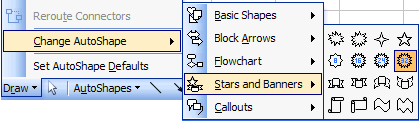
1. Change the shape / color of cell comments

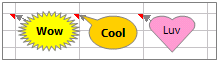
Just select the cell comment, go to draw menu in bottom left corner of the screen, and choose change auto shape option, select a 32 pointed star or heart symbol or a smiley face, just wow everyone 🙂

2. Filter unique items from a list

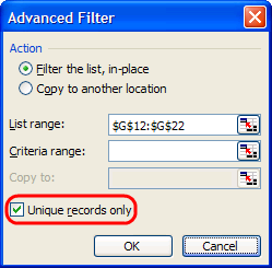
Select the data, go to data > filter > advanced filter and check the “unique items” option.

3. Sort from Left to Right

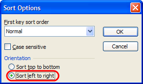
What if your data flows from left to right instead of top to bottom. Just change the sort orientation from “sort options” in the data > sort menu.

4. Hide the grid lines from your sheets

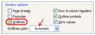
Go to Options dialog in tools menu, uncheck the “grid lines” option to remove gridlines from your worksheets. You can also change the color of grid line from here (not recommended)

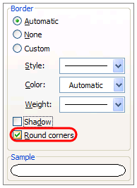
5. Add rounded border to your charts, make them look smooth

Just right click on the chart, select format chart option, in the dialog, check the “rounded borders”. You can even add a shadow effect from here.

6. Fetch live stock quotes / company research with one click

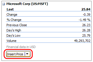
Just enter the stock symbol (MSFT, GOOG, AAPL etc.) in a cell, alt+click on the cell to launch “research pane”, select stock quotes to see MSN Money quotes for the selected symbol. You can fetch company profiles in the same way. Learn more.

7. Repeat rows on top when printing, show table headers on every page

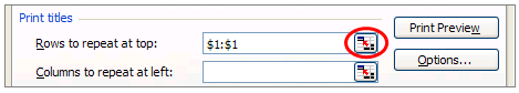
When you are on the sheet view, just hit menu > file > page setup, go to the last tab, specify “rows to repeat”. You can “repeat columns while printing” as well from the same menu.

8. Remove conditional formatting / all formatting with one click

Just go to Menu > Edit > Clear > All to remove all the formatting from selected cell / range.

9. Auto sum cells with one click

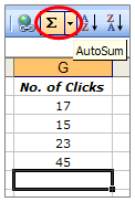
Select a bunch of cells and click on the Sigma symbol on the standard tool bar. Alternatively you can use Alt+= keyboard shortcut.

10. Find width of a column with formula, really!

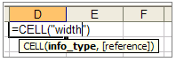
Just use =cell("width") to find the width of the column to which that formula cell belongs. Width is returned as the nearest integer.

11. Find total working days between any two dates, including holidays

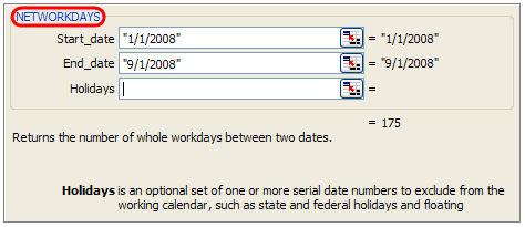
If you work on project plans, gantt charts alot, this can be totally handy. Just type =networkdays(start date, end date, list of holidays) to fetch the number of working days. In the above sample you can see the number of working days between New years day and September first of this year (labor day).

12. Freeze Rows / Columns in your sheet, Show important info even when scrolling

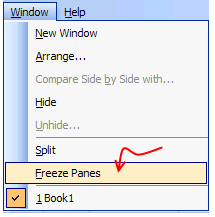
Select the cell diagonally beneath the row / columns you want to freeze (for eg. if you wan to freeze row 1&2 and columns A&B, click in C3), go to menu > window and click on freeze panes.

13. Split sheets in to two, compare side by side to be more productive

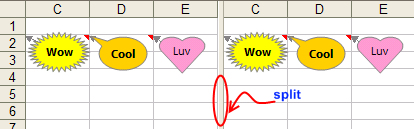
Just click on this little vertical bar on the bottom right corner of the sheet (see below) and drag it to create a vertical split. You can do the same way for a horizontal split as well 🙂

14. Change the color of various sheet name tabs

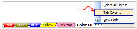
Right click on sheet and select “Tab color” option to change the worksheet tab colors. Group them with similar colors if you have lot of sheets, it looks nice.

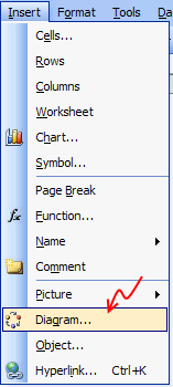
15. Insert a quick organization chart

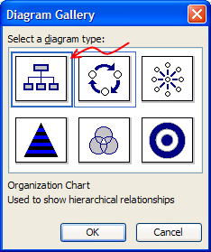
Click on menu > insert > diagram to open the above dialog, just select the organization chart option, enter node values and you have a pretty organization chart. Alternatively learn how to create org charts in excel.

So what do you say now? Isn’t Excel Exciting? 😀

Share this tip with your colleagues

Excel and Power BI tips - Chandoo.org Newsletter

Get FREE Excel + Power BI Tips

Simple, fun and useful emails, once per week.

Learn & be awesome.

121 Comments
Ask a question or say something…
Tagged under

cool, formatting, freeze panes, fun, how to, ideas, Learn Excel, microsoft, Microsoft Excel Formulas, spreadsheet, technology, tips, tricks
Category:

All Time Hits, Featured, hacks, ideas, Learn Excel

Welcome to Chandoo.org

Thank you so much for visiting. My aim is to make you awesome in Excel & Power BI. I do this by sharing videos, tips, examples and downloads on this website. There are more than 1,000 pages with all things Excel, Power BI, Dashboards & VBA here. Go ahead and spend few minutes to be AWESOME.

Read my story • FREE Excel tips book

Excel School made me great at work.

 5/5

Excel formula list - 100+ examples and howto guide for you

From simple to complex, there is a formula for every occasion. Check out the list now.

Calendars, invoices, trackers and much more. All free, fun and fantastic.

Power Query, Data model, DAX, Filters, Slicers, Conditional formats and beautiful charts. It’s all here.

Still on fence about Power BI? In this getting started guide, learn what is Power BI, how to get it and how to create your first report from scratch.

Related Tips

121 Responses to “Excel can be Exciting – 15 fun things you can do with your spreadsheet in less than 5 seconds”

Great tips! Another good one is highlighting a bunch of cells and changing the autosum visual at the bottom right to be Average or Count instead of auto sum.
[…] from a list, sorting data from left to right, freezing panes, and coloring your worksheet tabs. Excel can be Exciting : 15 Fun things to do with Microsoft Excel [Pointy Haired Dilbert — […]
[…] from a list, sorting data from left to right, freezing panes, and coloring your worksheet tabs. Excel can be Exciting : 15 Fun things to do with Microsoft Excel [Pointy Haired Dilbert — […]
Adam says:

one note on the «unique items» tip — this only works with numerical data — if you’re looking to weed out unique text entries, no dice — I work in Excel a lot with names and proprietary tags and would love a way to select a unique text entry — any suggestions?
- badOedipus says:
  
  You can filter duplicate text entries as described above if you use the advanced filter option, however it will not allow you to do an additional filter on an adjacent column afterwards without duplicating the data first.
  The method detailed below will allow you to filter our duplicate entries based on a conditional format.
  
  Select the range from which you wish to filter out duplicate text entries
  Click on Conditional Formatting > New Rule… > Use a formula to determine which cells to format
  type the following formula in the text box: =AND(COUNTIF(«RangeAddress«, «FirstCellAddress«)>1, MATCH(«FirstCellAddress«,»RangeAddress«, 0)<> ROW()) making sure to substitute accordingly. Note: RangeAddress should be absolute(«$A$1:$A$20»), and FirstCellAddress should be relative («A1»).
  Set the format to fill the cells with a color, depending on the application I use either a faint off-white to down play the color or a bright yellow to really make it pop — the choice is yours.
  Ta-da your duplicates are now colored. You can now filter by color if you use 2010 to see only duplicates or only unique records (unique being only one record per value). Pre-2010 you can sort by color to get them at the top/bottom of your list.
- Adrian says:
  
  Maybe if you use Access.
  - Vincent says:
    
    First post on chandoo.org, wahoooo!
    Anyways, after reading the above comments I just realized there’s a similar way to flag duplicate values with a formula, and one that works for strings as well as numbers. If you’re working in column A with a header row then your IDs will be in cells A2:A___. The following formula can be entered in B2 and filled downward to return FALSE when the ID is a repeated value, i.e. it is not the first instance of that value:
    «=MATCH(A2,$A$2:$A$__,0)=(ROW(A2)-ROW($A$1))».
    - Martin says:
      
      Re: =MATCH(A2,$A$2:$A$__,0)=(ROW(A2)-ROW($A$1))
      
      That’s a brilliant formula — I shall use that.
      
      Many thanks for sharing!
- Jason C says:
  
  Just highlight duplicates and then filter out the highlighted cells.
Mazy says:

OK, my hint, I think this excel function have never been documented or referred even in manuals:)

If you want to insert a part of a worksheet as picture (e.g. you want to include a small chart to a preformatted excel document), do the following:

DRAW anything, a square, circle, etc.
SELECT the cells you want to insert as a picture
SELECT the object you made (square,etc.)
PASTE

Voila:)
PK says:

I can’t get the comment to change. It just wants to draw a new autoshape.
- Tom says:
  
  To change the shape of the comment In Excel 2010 — I had to Customize the Ribbon [FILE, OPTIONS] and add a «Format» tab to the Main Tabs to allow the Format tab to be available all the time. Now I can Edit the shape.
@Adam.. It works for text data for me, which version of excel you are using, all these tips are tested in Excel 2003.

@PK … when you select comment to edit (shift+f2) click on the border of the comment, then go to bottom left corner in the screen and select draw > change auto shape. Should work in excel 2003 and above. Let me know if you see some problems 🙂
- Renate Callahan says:
  
  nope, it still doesn’t work. There is no draw -> change auto shape available for me. The left bottom corner of the screen just shows ‘Ready’ and if I right click on it it shows a lot of other things to activate, none of it is Draw or Auto options. I use Excel 2007
MM says:

You’ve missed an important step in your first tip. The Drawing toolbar must be active for this to work. Mine is not on by default, so I have to take the extra set to turn it on.
Jason says:

Very nice, thanks!

Could you clarify «You can also change the color of grid line from here (not recommended)» What is the recommended method.
The graphic designer-side of my job hates Excel, but the business owner side of me finds it to be essential. These tips help bring both sides (designer / business owner) closer together. Thanks!
@MM.. you are right, I have assumed the draw toolbar is on… thanks for pointing it out.

@Jason… “You can also change the color of grid line from here (not recommended)”, I said that to convey changing grid line colors is not recommended, as it can scare people or otherwise make your sheet look extremely busy… but you can change the color if you wish.. 😀
I use the NETWORKDAYS function all the time and it just blows people away.
Dude,
networkdays is my fav.

🙂
Nice post.

-Nikhil
My favorite excel command Ctrl and ~
displays all formulas
Thanks you pointy haired Dilbert, this is definitely a great list, like always bookmarked for future uses 😀
greats tips
i like command for displaying all formulas
thanks
Wade says:

Great tips!
However, #14 You need to right-click on the tab not the sheet.
#10 You can just left click and hold on the right most line of the column letter. Also, another tip a lot of users don’t know is that you can change a section of columns you want to one width by highlighting a column with the width you prefer and left-click-hold on the bottom right corner of that column letter and drag it through as many columns as you need.
Excel can be Exciting : 15 Fun things to do with Microsoft Excel | Pointy Haired Dilbert — Chandoo.o…

Who said Excel takes lot of time steps do something Here is a list of 15 incredibly fun things you can do to your spreadsheets and each takes no more than 5…
hey says:

Great history class. Should have gone for Excel 97 while you were at it 😉
0751firewire says:

Hey, HEY

Don’t be rude. It’s a waste of everyone’s time — including yours. Totally unnecessary.

******
Thanks for this post! I really enjoyed reading these tips. I will bookmark this post and will also subscribe to your weekly newsletter!

Thanks so much.
@Wade: you are right, you have to click on sheet name and not on sheet

and #10 was meant to show another way to find column width, but yeah, I always use the left click hold technique to see if the width is enough for me. Thanks for sharing it with everyone 🙂

@0751firewire: thanks 🙂

@everyone… I am happy so many of you liked this post and enjoyed these small but very useful stuff hidden away in the Excel.
- LEO DA VINCI says:
  
  Dear Chandoo,
  I have discovered you only 3 days back . I want a help from you . I am using a software which makes a grid file of lat,long and elevn. data (x,y,z) on 25m into 25m mesh size . I feel that this grid file which is made from a xcel csv sheet containing random x,y,z points can be made on xcel sheet itself. Can i do that ? example of a source data shown below
  
  x y z
  100 50 12.5
  200 40 14.0
  220 75 12.0
  202 60 15.0
  - @Leo Da Vinci
    You can either import and existing CSV file or setup the file directly in Excel as a workbook
  - whatever says:
    
    You can not make a grid gragh on xeel because it has boxes you would have too get speacial advanced software like the sciencestes do:
    
    i know more that somebody from the GEEK squad!!
    - @Whatever
      Can you post a sample of a Grid Graph or a link where we can see what your referring to?
[…] Excel can be Exciting : 15 Fun things to do with Microsoft Excel | Pointy Haired Dilbert — Chandoo.o… […]
Tip #13: In case anyone is an excel newbie like me, to remove the new vertical bar, just double click on the bar.
- Rufus says:
  
  Thanks fir the tip re vertical bar.
  I am a baby Excel beginner at 86!!!!!
Roger says:

Unique text entries can be found easily — use COUNTIF function for each row. You can use autofilter to delete anything with result > 1.
LD says:

To the person joking about Excel 97 — that version of Office is still the standard at my workplace. No joke.
[…] Excel can be Exciting : 15 Fun things to do with Microsoft Excel | Pointy Haired Dilbert — Chandoo.o… […]
shivshankar says:

Adv
[…] Find total working days between any two dates, including holidays […]
Arti says:

I tried second tip to remove the duplicate entries from the row by copying it in another location but its not working if I use data in A’ th column as

A1 aa
A2 aa
A3 bb

and I am trying to copy the unique records to column B.
The above scenario is not working if duplicate entries are present in A1 and A2.
It will work if duplicate entries are present below first record.
Robert says:

@Arti

Autofilter as well as advanced filter needs titles of the columns in the first row. If you have only the three items in your list, Excel assumes, the first «aa» is the title (field name) of your list, not an entry in the list itself. As a result, Excel writes into column B again the first aa as the title and the second aa and bb as the 2 entires.

Simply insert a row above your list and give your list a name in cell A1. Then it should work.
[…] more than 5 seconds to do. Happy Friday 1. Change the shape / color of cell comments Just select thhttp://chandoo.org/wp/2008/08/01/15-fun-things-with-excel/MI-INFO Tutorials — Excel BasicsFor large worksheets that span more than one screen of […]
[…] Excel can be Exciting : 15 Fun things to do with Microsoft Excel […]
[…] on September 13, 2008 Few weeks back, I came across a post about some useful tips in MS Excel — Excel can be exciting . So, I thought I’ll collate some of the helpful tips and tricks that I’ve come across while […]
[…] 15 Fun things you can do with Excel […]
Melli says:

Nr. 5
-> does not work. And I have Excel 2003!
@Melli .. Welcome to PHD…

Are you sure rounded borders are not working. I have made this example in Excel 2003 and they are working alright for me. You have to select the entire chart to change borders to rounded, not the plot area alone.
[…] Excel can be Exciting : 15 Fun things to do with Microsoft Excel | Pointy Haired Dilbert — Chandoo.o… (tags: work windows useful tutorials tutorial tricks toread tools) […]
[…] But often we leave the last steps for manual processing. The article addresses one such problem (extracting unique cells from a range) and tells us how we can automate the whole […]
homepage templates…

I just wanted to share this nice address, where you can get wordpress themes for free. I use one of the designs for my own blog and it was really easy to install. Just activating it in admin and the job was done. :-)…
I did not know excel is this much fun.
Ketan says:

@ Adam & Chandoo…
For removing / filtering the duplicate entry / unique data…one can use the readymade menu from JMT utilities….very useful…
[…] Using Advanced Data Filter […]
[…] Excel can be Exciting — 15 fun things you can do with excel […]
rayna says:

Thx so much PHD…tusi gr8 ho ji…:)
[…] > and un-check grid lines option. (Excel 2007: office button > excel option > advanced)… Get Full Tip 50. To hide a worksheet, go to menu > format > sheet > hide… Get Full Tip 51. To align […]
[…] Beautiful City Photography» and «10 Companies Hiring for Work from Home». (They’ve also included «15 fun things to do with Microsoft Excel», which may be the most terrifying title in blogging […]
[…] Learn Excel Formulas in Plain English | Executive Dashboards in Excel — 4 Part Tutorial | 15 Excel Fun Tips […]
[…] Related: How to change the shape of cell comments from rectangle to any other shape […]
[…] Learn how to color excel worksheet tabs. […]
[…] on excel comments: change the shape of excel comment box | pimp your comment boxes | extract comments using […]
Francis says:

i cannot find CHANGE AUTO SHAPE option in Excel 2007 to design my comment box. Please help?
- @Francis… Excel 2007 has made it little difficult to change comment shapes, but it is still possible. First add a regular shape (like rectangle) to the worksheet. Now select it. This will show a new ribbon called «format». From here, you can find the change shape tool. Add this tool to Quick Access Bar.
  
  Now Select the comment cell and edit comment. At this point, use the change shape tool from QAT to change the shape of comment.
  - Renate Callahan says:
    
    all right!! Thanks, this answers my question posted above. Yes, now it does work and it looks great! 🙂
Ken Buffong says:

Its really made easy.
Paul says:

Its a bit of a faff in 2007, not sure if its just my work computer than won’t let me change the default shape for comment boxes… But for this one workbook i’ve added a simple:

ActiveCell.Comment.Shape.Select
Selection.ShapeRange.AutoShapeType = msoShapeVerticalScroll

Or you can change msoShapeVeriticalScroll to any shape you like…
VENKATRAMAN V S says:

Dear All

Thank you all very much. You guys have taught me a lot of new things in Excel. Keep continuing the good work.
nazia says:

thanx so much…it really is of gr8 gr8 help to me…… :))
The color sheet tab option has disappeared. Was there and working fine but now when I right click there isn’t an option to change the color of my sheets. How can I get this option back?
- @Deanna.. you can reach this from Format button on home ribbon. Key board short code — ALT + HOT (just press h,o and t one after another).
Sanjay says:

Hello,

Can I know the name of the last person who saved the file last.

In a team of 10 members working on a shared excel file, this information will help me to know the name of the person who modified the file.
Shouvik says:

@Sanjay: Open the workbook — Click on File -> Properties -> Click on the Statistics Tab for the information you are looking for.
mer says:

Wish I could see those images, because they’re now blocked by photobucket. Next time use imgur, or host it on your own server.
mimi says:

Brilliant!
Helped me teach my pupils loads in I.C.T today!
LOL
irha says:

you don’t have references 🙁
Hussein says:

I liked a lot this web site

thanks
Rahul aggarwal says:

@chandoo ji
can we change default comment cell box shape in excel 2007or 2010?
saravanan says:

Hi Friends

Can we Increase the Column width >500 in excel 2003.

Pls help…
losraiders says:

I really like tip #1 but I’m how can you do it if you’re using Excel 2007. I don’t see the drawing toolbar…I believe it’s gone in 2007 but not certain. I did see the autoshape when I select the commnent and right click but nothing happens when I select it.
- This is possible in Excel 2007 (and 2010) too. Follow below steps:
  1. Add any drawing shape.
  2. Select it and go to format ribbon
  3. Right click on Edit shape and add it to «Quick Access toolbar»
  4. Now, remove the shape
  5. Select comment cell.
  6. Edit comment.
  7. Use quick access toolbar to change the shape to anything you want.
  - Sudhir says:
    
    This is awesome Chandoo ! Tip#1 I was most impressed. #6 I was not able to replicate — if you meant Alt + (Mouse left) click, it did not work. But manually triggered the reference — but was unable again to make it available as embedded «auto look up» in the sheet itself.
steve says:

wow! this site is awesome
Some tricks are not working with Excel 2003

But others are too cool thanx
[…] and un-check grid lines option. (Excel 2007: office button > excel option > advanced)… Get Full Tip 50. To hide a worksheet, go to menu > format > sheet > hide… Get Full Tip 51. To […]
[…] Using too many tab colors on your excel workbooks [how to do this] […]
Can anyone help. I want to be able to hide a row for exampe row A if the Cell A1 is empty after i have sorted the rows.
I can write the macro to sort the list then I am stuck.

Any HELP OUT THERE.

Regards ken
why isnt my thing working
=NETWORKDAYS(«11/11/2011″,»12/12/2012»,[holidays])
- D Gamlath says:
  
  It’s not going to work that way. At least not with the parentheses. Try entering the two dates in two cells and referring those cells within your formula 🙂
- Sudhir says:
  
  It will work — a date in formula is entered as follows:
  =NETWORKDAYS(DATE(2011,11,11),DATE(2012,12,12),0)
Marcia Fay Cobb says:

I’m doing an address directory. All I want to do is find out how to delete a blank line or move the second line up to the first line in the cell? Appreciate any help you can give. Thanks.
Shivani says:

How to make comments of different shapes in Excel 2010?
Jignesh says:

we have shared the workbook, so other user can access and feed data at their respective fields, all user can view list of users accessing the shared file,but unfortunately if a user removed from list of user name then that user will be disconnected and whatever changes made will be proved to be useless as file become exclusive.

Could you please anybody help me out how to protect the username list so nobody could removed from the list.
Abdul Azeez says:

how to change font color in cell by using formula
- Sudhir says:
  
  This can be done using conditional formatting. Is there a specific thing that you are looking at ?
Nadalvski says:

Hi Chandoo,
I bumped into your site two days ago and am hooked to it.
Very helpful and elaborate articles.
Thanks.
[…] Check out why here. […]
Prakash says:

Can anyone help me to do the following:
Is there any option to copy all the procedures done for a set of values to other set of value which we will input in later stages.
In other words: Imagine I have a list of values(first set) for which I need to do some mathematical and logical operations and I will get the final required output.

Also if I have one more set of values(second set) for which I need to do the same procedure to get required output.
So my question is : Is there any way to get the final output directly for set-2 values based on the steps(procedures) done for set-1 so that it will reduce lot of work.

Please help me.
Thank you all.
- @Prakash
  
  Can you ask the question in the forums
  http://chandoo.org/forum/
  Please also attach a sample file with an example of what results you want
nmsdfmn says:

whey it is appearing
Kris says:

I think you should mention that this feature available from WHAT Version otherwise users go crazy!
extreme x says:

Oh very cool stuff! Thanks
Rushabh Gala says:

This is really a good article even I read some comments which were really useful.
Chirag Parmar says:

That was cool Sir. Thanks for sharing these tricks with us.
Dustin says:

Help!! I just pulled data out of a different software and pasted values only in excel. Anything with a character other than a number is shifted to the left of the cell. Anything with only numbers is shifted to the right of the cell.

The VLOOKUP is only working on the ones shifted to the right. The formatting on the home tab is all the same. Why is it working on some but not the others? Is there underlying format that can be erased??
- Dustin says:
  
  The VLOOKUP is only working on the ones shifted to the left.********
  
  (Only works for cells that have characters other than numbers, in addition to numbers)
thanks for your tips and tutorials excel for children… i like
sandeep kothari says:

Hat tip to you, OSUM Chandoo!
Sandy says:

I’m adding birthdates to a column. I need to know how to differentiate a birthdate in the 19 hundreds (19XX) from a birthdate in the 2 thousands (20XX).

I appreciate any help!!! Thank you
Chad Estes says:

Assuming your birth date column is G and is a date datatype:

=if(YEAR(G1) < 2000, «Born in 20th Century», «Born in 21st Century»)
Sagar says:

Is there any way that, I can overlap and compare between two worksheets. This is required in case to auto highlight edited data between the copies. Please help….
Nice post . Step -> 7. Repeat rows on top when printing, show table headers on every page — will be useful . Thank you.
Bhanu Prasad K S says:

Hi Chandoo,

Firstly, I wanted to say a big thank you for whatever you are doing for people like me who need knowledge of excel and power BI.

I wanted to know how we can highlight cells which have dates between the given range.
for example, i want to highlight cell which have dates between Jan 1, 2022 and June 30, 2022.

Источник

An Excel spreadsheet is a very powerful software which was developed by Microsoft in 1985 and is used by over 800 million users for number crunching, data analysis & reporting, charting and note taking – wherein its true power is often underutilized 🙂

It is widely used by organizations for calculating, accounting, preparing charts, budgeting, project management, and various other tasks. The different uses of an Excel spreadsheet is in fact limitless! In this tutorial we will hold your hand and teach you how to use Excel for the first time.

Want to know How To Master Excel from Beginner to Expert?

*** Watch our video and step by step guide below with a free downloadable Excel workbook to practice ***

Watch it on YouTube and give it a thumbs-up!

An Excel Spreadsheet is the go-to software to analyze, sort, or present a large amount of information and data in no time.

In this Excel tutorial, I will cover the Basics of Excel that you need to know to get started with how to use Excel. This Excel for dummies guide will include tutorials on:

Opening an Excel Spreadsheet
Understanding the Different Elements of an Excel Spreadsheet
Entering Data in an Excel Spreadsheet
Basic Calculations in an Excel Spreadsheet
Saving an Excel Spreadsheet

Let’s start this step by step Excel tutorial on – “How to use Excel”

Opening an Excel Spreadsheet

To open an Excel Spreadsheet, follow the steps of this Excel tutorial below:

Step 1: Click on the Window icon on the left side of the Taskbar and then scroll below to find “Excel”.

Step 2: You can either click on the “Blank Workbook” button to open a blank Excel spreadsheet or select from the list of pre-existing templates provided by Excel.

To open an existing Excel spreadsheet, click on the “Open Other Workbooks” and select the Excel sheet you want to work on.

Step 3: An Excel spreadsheet is now opened and you are ready to explore the wonderful world of Excel.

Understanding the Different Elements of an Excel Spreadsheet

To explore the different ways on How to use Excel you should be familiar with the different elements of Excel first.

Excel Workbook and Excel Worksheet are often used interchangeably, but they do have different meanings. An Excel Workbook is an Excel file with the extension “.xlsx” or “.xls” whereas an Excel Worksheet is a single sheet inside the Workbook. Worksheets appear as tabs along the bottom of the screen.

Now that you are clear about these two terms, let’s move forward and understand the layout of an Excel Spreadsheet. It is a crucial step if you want to know how to use Excel efficiently.

Excel Ribbon

The Excel Ribbon is located at the top of the Excel Spreadsheet and just below the title bar or name of the worksheet. It comprises various tabs including Home, Insert, Page Layout, Formulas, Data, etc. Each tab contains a specific set of commands.

By default, each Excel spreadsheet contains the following Tabs – File, Home, Insert, Page Layout, Formulas, Data, Review, and View.

File Tab can be used to open a new or existing file, save, print, or share a file, etc.
Home Tab can be used to copy, cut, or paste cells and work on the formatting of data.
Insert Tab can be used to insert the picture, charts, filter, hyperlink, etc.
Page Layout Tab can be used to prepare the Excel spreadsheet for printing and exporting data.
Formula Tab in Excel can be used to insert, define the name, create the name range, review the formula, etc.
Data Tab can be used to get external data, sort filter and group existing data, etc.
Review Tab can be used to insert comments, protect the document, check spelling, track changes, etc.
View Tab can be used to change the view of the Excel Sheets and make it easy to view the data.

You should be familiar with these tabs so you can understand how to use Excel efficiently. You can even customize these Tabs using the following steps:

Step 1: Right-click on the ribbon and click on “Customize the Ribbon”

Step 2: An Excel Options dialog box will open, click on the New Tab.

Step 3: Select that newly created tab and click on Rename and give it a name e.g. Custom

Step 4: Now you can add the commands that you want under each group by simply clicking on the command from the Popular Command column and click on Add >>

This will create a New Tab called “Custom” with a popular command “Center“.

Under each Tab, there are various buttons grouped together. For Example – Under the Home Tab, all font-related buttons are clubbed together under the Group name “Font”.

You can access other features related to that group by clicking on the small arrow at the end of each Group. Once you click on that arrow, a dialog box will open and you can make further edits using that.

There is also a search bar available next to the tabs which was introduced in Excel 2019 and Office 365. You can type the feature that you are after and Excel will find it for you.

You can also collapse the ribbon to provide extra space in the worksheet by pressing the keyboard shortcut Ctrl + F1 or by right-clicking anywhere on the ribbon and then clicking “Collapse the Ribbon”.

This will collapse the Ribbon!

Formula Bar

Excel’s Formula bar is the area just below the Excel Ribbon. It contains two parts – on the left is the name box (it stores the cell address) and on the right is the contents of the currently selected cell. It is used to type values, text or an Excel formula or function.

You can hide or unhide the formula bar by checking/unchecking “Formula Bar” under View Tab.

You can also expand the formula bar if you have a large formula and its contents are not entirely visible. Click on the small arrow at the end of the formula bar and it will be expanded.

Status Bar

At the bottom left side of the workbook, all the Excel worksheets are shown. You can access an Excel sheet by simply clicking on it.

To add more Excel sheets, click on the “+” sign below which will add a new blank Excel sheet.

You can reorder the Excel sheets in your workbook by dragging them to a new location with your left mouse button.

You can also rename each Excel sheet by Right Clicking on a Sheet Name > Click on Rename > Type the Name > Press Enter.

At the bottom right of the Excel spreadsheet, you can quickly zoom the document by using the minus and plus symbols. To zoom to a specific percentage, in the ribbon menu go to the View tab > Click Zoom > Click on the specific percentage or type in your custom % > Click OK.

There are different Excel workbook views available at the left of the zoom control: Normal View, Page Break View, and Page Layout View. You can select the view as per your choice.

Cell & Excel Spreadsheet Basics

Any information including text, number, or an Excel formula can be inserted within a Cell. Alphabets are used to label Columns and numbers are used to label Rows.

An intersection of a Row and Column is called a Cell. In the image below, cell C4 is the intersection of Row 4 and Column C.

You can refer to a series of cells as a range by putting a colon between the first and last cells within the range. For example, the reference to the range starting from A1 to C10 will be A1: C10. This is great when you are using an Excel formula.

Now that you are familiar with the different elements in an Excel Spreadsheet, let’s show you how to use Excel to enter data and do some calculations!

Entering Data in an Excel Spreadsheet

Follow this step -by-step tutorial on how to use excel to enter data below:

Step 1: Click the cell you want to enter data into. For Example, you want to enter your sales data and want to start with the first cell, so click on A1

Step 2: Type what you want to add, say, Date. You will see that the same data will be visible on the Formula Bar as well.

Step 3: Press Enter. This will store the written data on the selected cell and move the selection to the next available cell, which is A2 in this example

To make any changes in the cell, simply click on it and make the changes.

You can copy (Ctrl + C), Cut (Ctrl + X) any data from one Excel worksheet and paste it (Ctrl + V) to the same or another Excel worksheet.

Basic Calculations in an Excel Spreadsheet

Now that you have understood how to use Excel to enter data, let’s do some calculations on the data. Let’s say you want to add two numbers: 4 and 5 in the excel spreadsheet.

Follow the steps below on how to use Excel to add two numbers:

Step 1: Start with the = or the + sign to tell Excel that you are ready to run some sort of calculation.

Step 2: Type number 4.

Step 3: Type + symbol to add

Step 4: Type number 5.

Step 5: Press Enter.

You will see the result 9 is displayed in the cell A1 and the formula is still displayed in the formula bar.

Let’s try to use a cell reference to make calculations.

In the example below, you have Column A that contains the number of products sold and Column B that contains price per product and you need to calculate the total amount in Column C.

To calculate the total amount, follow the steps below:

Step 1: Select cell C2

Step 2: Type = to start the formula

Step 3: Select cell A2 with your mouse cursor or by using the left arrow key.

Step 4: Type the multiplication sign *

Step 5: Select cell B2

Step 6: Press Enter

You can use various calculation operators, such as Arithmetic, Comparison, Text Concatenation and Reference operators that will be useful for you to have a clear and complete idea on how to use Excel.

Here is a walk-through for Excel for Dummies by Microsoft covering the most requested features of Excel.

Saving an Excel Spreadsheet

To save your work in Excel, click on the Save button on the Quick Access Toolbar or press Ctrl + S.

If you are trying to save a file for the first time, then follow these steps:

Step 1: Press Ctrl + Shift +S or Click on the “Save As” button under the File tab.

Step 2: Click on “Browse” and choose the location where you want to save the file.

Step 3: In the File name box, enter a name for your new Excel workbook.

Step 4: Click Save

Here is an Excel for Dummies Video from Microsoft explaining how to save an Excel Workbook.

This brings us to the end of this how to Use Excel tutorial.

I have just covered the basics of how to use Excel in this article. As an Excel newbie, Excel is a completely unexplored & exciting world for you right now and you are going to learn so much along your journey.

My advice is to take baby steps, learn how to use one Excel feature, apply it to your data, make mistakes and keep on practicing.

Within 7 days your Excel confidence will skyrocket!

Make sure to download our FREE PDF on the 333 Excel keyboard Shortcuts here:

You can learn more on how to use Excel by viewing our FREE Excel webinar training on Formulas, Pivot Tables and Macros & VBA!

You can follow our YouTube channel to learn more about How To Use Excel for Dummies!

👉 Click Here To Join Our Excel Academy Online Course & Access 1,000+ Excel Tutorials On Formulas, Macros, VBA, Pivot Tables, Dashboards, Power BI, Power Query, Power Pivot, Charts, Microsoft Office Suite + MORE!

Источник

Tools, Calculators and Simulations
Dashboards and Reports with Charts
Automate Jobs with VBA macros
Solver Add-in & Statistical Analysis
Data Entry and Lists
Games in Excel!
Educational use with Interactive features
Create Cheatsheets with Excel
Diagrams, Mockups, Gantt Charts
Fetch live data from web
Excel as a Database

Excel is one of the most used software in today’s digital world. Most people quickly open up an Excel file when they need to write or calculate anything. It is like “paper”. (remember those graph notebooks from school times..)

Good old days..

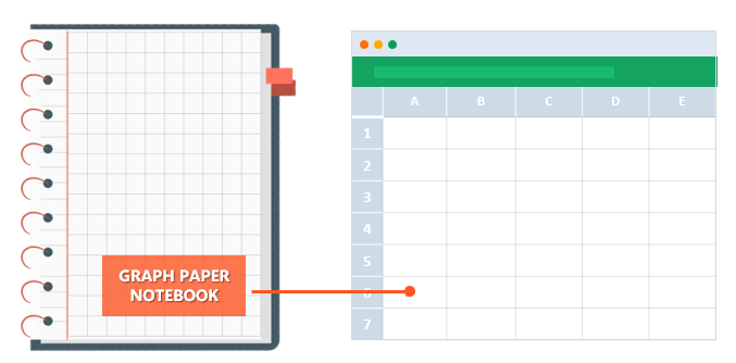
Actually, this is not only specific to Microsoft’s Excel but most of the spreadsheet software like open office or google sheets. However, we will focus on Excel and what can you do with it today, as it offers huge flexibility you will discover below.

Let’s start with the main usage areas of Excel. As we all know, spreadsheets are designed to make calculations easier. So they contain “formulas”. They allow us to make basic math like summing, multiplying, finding average as well as advanced calculations like regression analysis, conversions, and so on.

When we combine these powerful math features with some tables, lists, or other UI elements, we can come up with a calculator. And most of the time they will be dynamic (meaning that when you change a parameter all the rest of the calculations will adapt accordingly)

Below see an example from our past studies as Someka:

For more details, check Someka – Custom Services

We have built this calculator for an app development company executive. He was changing the parameters he wants and sees the outcomes immediately.

This is great especially when you try to make big “models” in excel. Financial Modeling is one of the most used application areas of these big models. If we tried to do this with pen-paper (which used to be the way once upon a time) it would be horrible I guess:

Financial Modeling with Excel Evolution

Financial modeling is also being used to test the excel skills of experts. They even make a competition for it: ModelOff

We also have a tool for startups to make a feasibility study playing with their own variables:

This is a comprehensive Feasibility Study Excel Template for app startups with download projections, costs, financial calculations, charts, dashboard, and more.

The business world is demanding. It is not enough just to make the calculations, set up your tables, and write the text. You have to create pie charts, trends, line graphs, and many more. Whether you are getting prepared for your pitch or make a presentation in your company, you can use Excel’s chart features.

Reports and Charts in Excel

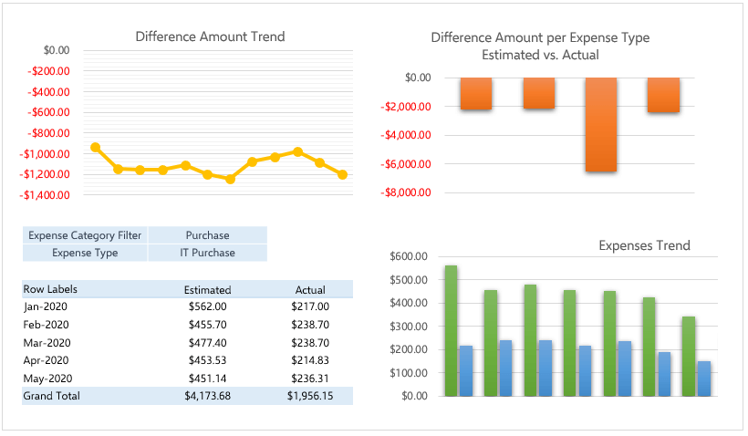
Pivot Tables

One of the greatest features which Excel offers is Pivot tables. This is an advanced Excel tool that helps you create dynamic summary reports from raw data very easily. After you create your table you can play with parameters easily with a drag and drop interface.

It looks like this:

Pivot Tables are quite useful

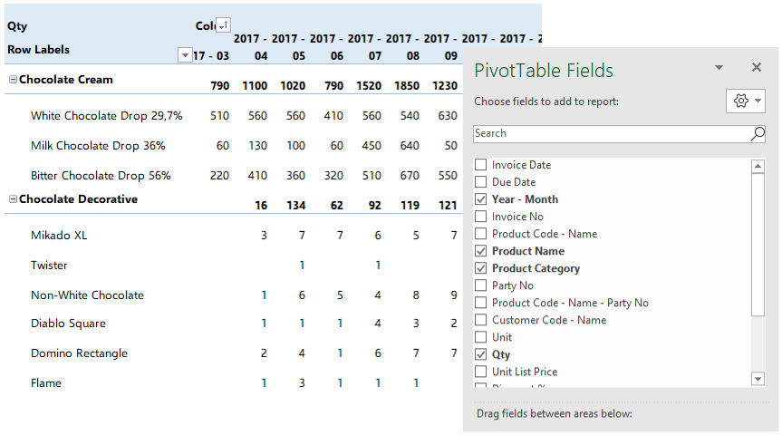
Dashboards

Complex excel models do have lots of variables, calculations, and settings. And instead of managing all variables one by one on different sheets, different places it is a very good idea to put them together like a “control panel”.

You can think dashboards as cockpits of planes.

Recently dashboards became very popular. There are lots of training videos about how to build and design control panels for our excel models. Actually, they are not so different from the rest of the calculations.

But the main idea is: if there is something you may want to change, later on, don’t write it directly in the formula but bind it to a variable.

Let’s say you are building a sales report for your manager. He asks you to make the file changeable so that he can see the results in US dollars or Euros according to the situation. Instead of writing an Fx rate into the calculations, you should bind this to a cell that you can play with later on.

Like this:

Excel Dashboard Logic

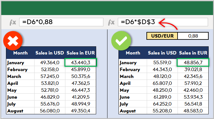
This may seem so obvious to some of you. But this is the basic approach of all dashboards in excel files. Of course, you can improve it with more complex formulas, buttons, cool charts, and even VBA but the main idea stands still.

Here is an example of a complete set of the dashboard:

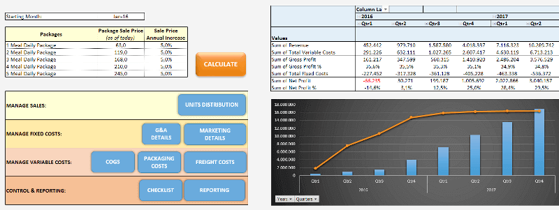
Excel Dashboard from Someka Custom Services

Or a dashboard for a livestock feasibility study:

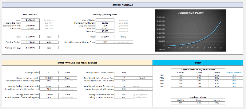
Livestock Feasibility Study Dashboard

If you are interested in Sales Dashboards, you may want to check out our Excel template:

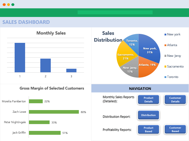
This is an interactive Sales Report Template in Excel. Features a dashboard with profitability, sales analysis and charts.

Other than that, Marketing ROI Calculator would be very helpful to prioritize your marketing campaigns in Excel:

It will provide essential metrics and help you to manage all your marketing campaign channels in one place.

Most of the users who use Excel extensively are already coding. But if you ask them whether they know how to code most probably they will say no. Of course, writing formulas is a very small part of the things you can do with VBA. It is a strong programming language that lets you create small scripts (macros), user forms, user-defined functions, add-ins, and even games! (which we will touch below separately)

I will not dive into VBA here since it is a detailed area. But there are some basic things that will be beneficial to know for those who use Excel often:

You can record macros for repeating jobs: You don’t need to code from scratch. Just click on the record macro button and it will write the code for you in the background. (If you want, you can modify later on)
It extends the borders of Excel world. If you feel like you are limited somehow in Excel, you are more like an advanced user. It is time to get a little bit into VBA.
You can create user forms with VBA only. If you see something like this, know that it is using VBA:

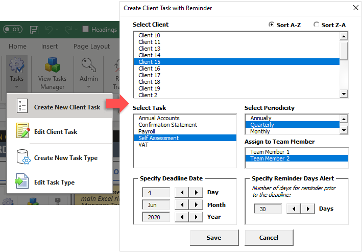
Someka Client Task Management Template

VBA is quite powerful and if you work with Excel extensively you won’t regret learning a bit. For example wouldn’t it be nice if you could send bulk emails from an Excel spreadsheat with a button click?

It is not surprising for spreadsheet software like Excel to offer advanced math techniques to make more complicated studies. (To be honest, I am not a statistics expert but with an engineering background, I will try to do my best to explain the basics. Feel free to correct me if I’m wrong)

Data analysis is a trending concept for recent years with the development of powerful computers and improved software. We are collecting and recording much much more data compared to the past. Take a look at this chart to understand what I mean:

Source: Statista

Especially this part:

“more data has been created in the past two years than in the entire previous history of the human race”

It is a bit frightening, isn’t it? Ok, we are not going to dive into the “Big Data” world. Let’s get back to our humble excel world.

As we collect this much data, some people will want to analyze it. Otherwise, it makes no sense to spend billions of dollars on those data centers. Excel has built-in functions for basic descriptive statistics methods like Mean, Median, Mode, Standard Deviation, Variance etc.

But if we want to go a bit further I will mention two Excel features (actually add-ins) at this step: Solver and Regression Analysis

Solver

Have you ever heard of “optimization”? When we have more than one parameters that affect the outcome, we can only have a most optimized solution rather than a maximum solution. This may sound weird but it is very valid in our daily lives.

One of the simplest and popular examples is: Farmer Fence Optimization Problem

“A farmer owns 500 meters of the fence and wants to enclose the largest possible rectangular area. How should he use his fence?”

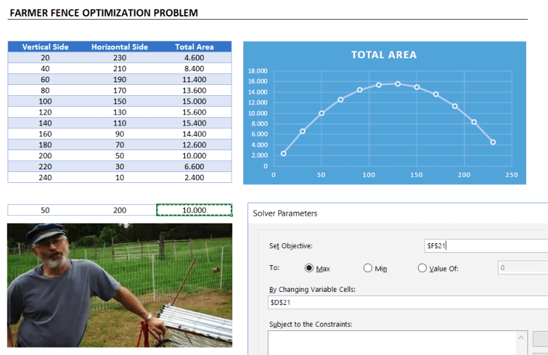
Farmer Fence Optimization Problem Excel Solver Solution

This is a very simple example to explain what a solver does. But actually, you can run much more complicated data sets with Solver.

Regression Analysis

Since this is a bit advanced topic for this blog post, I will only touch the surface.

In most simple terms, regression analysis helps you find the correlation between the variables. For example, you may want to know what is the relation between the number of birds flown over your head and the money you earned today. (sorry for the silly example. No, I am not curious about it You will need to gather sample data and put in an analysis to see if there is any correlation.

It seems something like this:

You put your data:

Sample Data

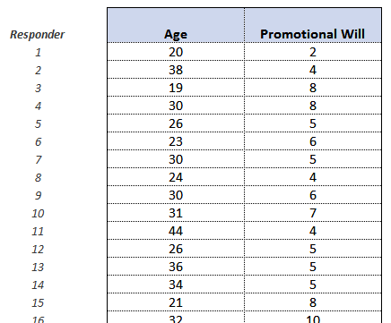
Run the regression from Analysis Toolpak:

Analysis ToolPak Excel

And get results something like this:

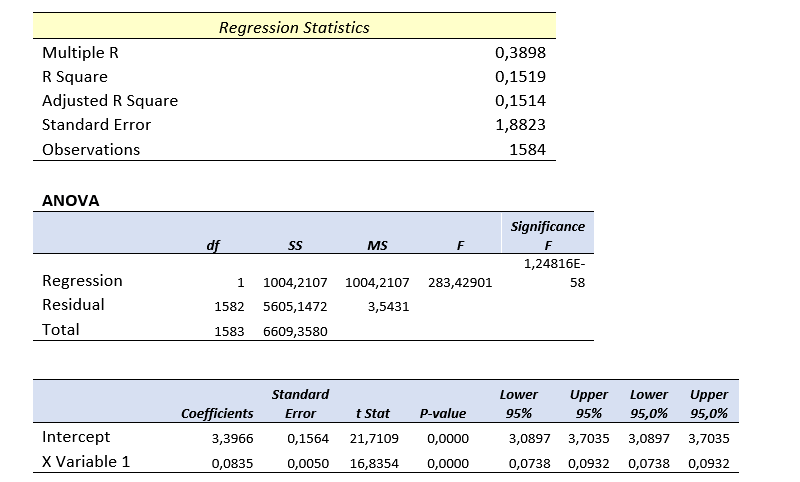
Excel Regression Analysis Results

Of course, there is much more sophisticated software to run data analysis. However, there is a joke in business intelligence communities:

What is the most used feature of any business intelligence solution?
It is “Export to Excel”

Looks like we won’t stop using Excel anytime soon.

Coming back from boring data analysis world, let’s mention the simplest and most handy usage area of excel: Make Lists!

It is already self-explaining so I won’t bother with the details. When you want to list down some simple data, take notes, create to-do lists, or anything. Just open the excel and write it down. Did we mention that “paper alternative” thing? Oh yes, we did.

A lead list example:

Lead List in Excel

You can also convert PDF files into Excel files in order to make it easier to work on. This can be done automatically with some software. But some pdf files cannot be processed automatically (like handwritten documents, scanned invoices, etc). You will need to do it manually.

PDF to Excel

When you want to play with the data on a web page, you can easily copy-paste it into an excel file and then you can sort, filter or do anything you want:

For example, Fortune 500 US List:

Fortune 500 List in Excel

Everybody loves to-do lists. And we have created useful to-do list in Excel for business or personal uses. Check it out, it is free:

To-Do List Excel Template

We already mentioned this in the VBA section above. But it is worth to talk a bit more.

Visual Basic allows you to code complex things like games as well. But of course, don’t expect a GTA or FIFA. Things like chess, sudoku, or Monopoly is OK. But, a few people have gone far and created more complicated things, like an RPG game. Take a look at this:

Source: carywalkin.ca

This game has been created by an accountant, Cary Walkin. I know it doesn’t look great but it is in Excel! (you can play it at the office )

Another example:

Source: excelunusual.com

A flight simulator in Excel?? Is it the same thing we use to sum up the sales figures? Lol yeah.

You can also embed flash games into Excel (like Super Mario, Angry Birds or whatever) But I count them off as they are not built with VBA.

As we mentioned in the Financial Modeling section, Excel is quite good for creating dynamic results according to the inputs. We get the benefit of this to create interactive tools.

One example that comes to my mind is this spreadsheet, guys from San Francisco have prepared:

Source: exceleverest.com

I haven’t tried it myself but an Excel tutorial in Excel. Liked the idea!

Another similar interactive Excel learning tool is from Keyskillset:

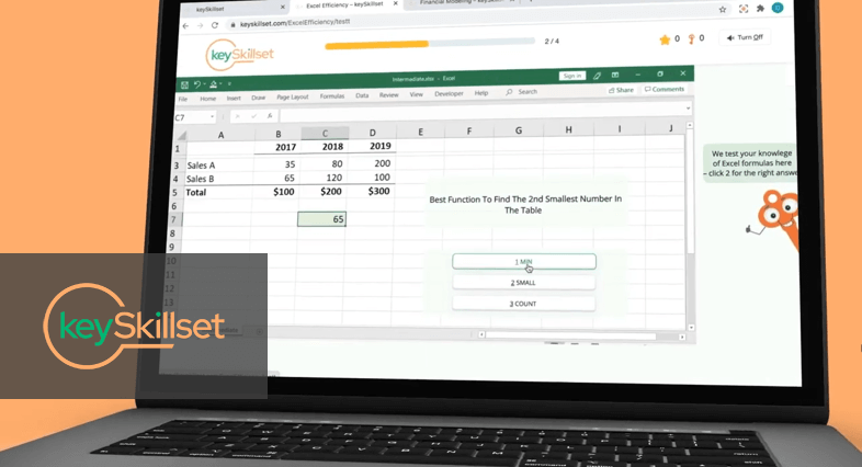
Actually, this is not completely in Excel and works as separate software but I liked how they combine the Excel training with gamification features.

Quizzes are good tools for interactive learning and you can prepare in Excel as well. A quizmaster template from indzara.com:

Source: indzara.com

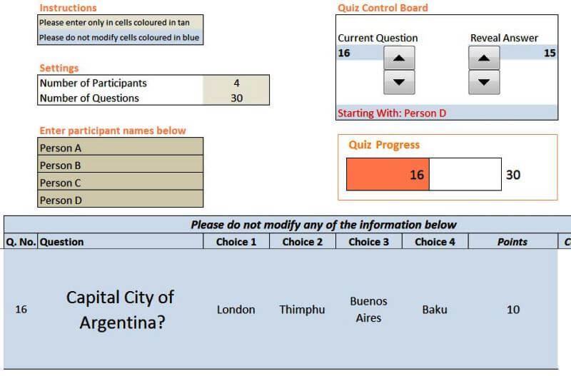
A student lesson plan template in excel which we have prepared recently:

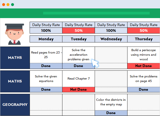
Someka Student Lesson Plan in Excel

You can learn Excel in Excel!

As said: Practice Makes Perfect!

You can test your Excel skills in Excel with Excel Formulas Trainer:

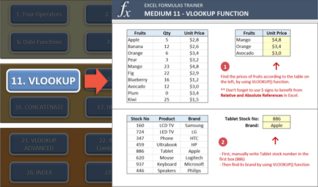
This is actually an Excel template prepared with VBA macros and basically works as a practice worksheet. It has 30 sections and around 100 questions. You can learn VLOOKUP, IF and much more excel formulas by doing. If you like the idea of “learning by doing”, then it is worth to check.

Also, this online course from GoSkills is for everyone as well, covering beginner, intermediate and advanced lessons.

By cheat sheets, we don’t refer to the piece of paper with information written down on it that an unethical person might create if they weren’t prepared for a test. What we mean is a reference tool that provides simple, brief instructions for accomplishing a specific task. We use this term because it is highly popular recently.

For example, this is a cheat sheet:

Created by Jacob Seidelin

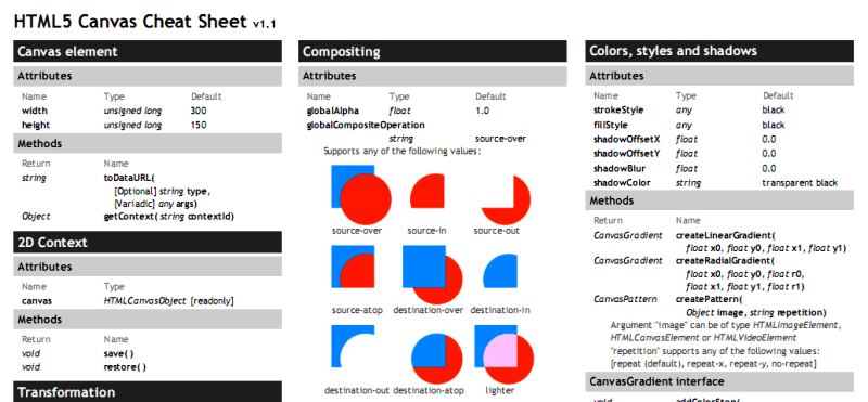
This compacted and summarized info is very useful in many aspects. When you try to memorize things, lookup, reference, etc. And can be easily created with Excel. Let’s make a Google search for a cheat sheet made in Excel.

This one is from Dave Child (cheatography.com) and I was also using this one I first learned HTML:

Created by Dave Child

The last example is an Excel Cheatsheet made for Excel shortcuts:

Of course, if you are looking for stylish infographics and cheat sheets, you should check out design software.

I know Excel is maybe not the best tool to do these. There are great programs or websites to make mockups, diagrams, brainstorming, mind-mapping, or project scheduling. But there are habits as well. Even though I am very open to try and use these kinds of brand-new tools, I find myself using excel for a mockup or a mind map. (select shapes, put notes, put arrows, change colors etc. Omg it is tedious)

Gantt charts can be a bit old-school as agile project management methods are increasing in popularity, they are still being used widely. There are several Gantt chart excel templates on the web.

A Gantt chart example from vertex42.com:

Source: vertex42.com

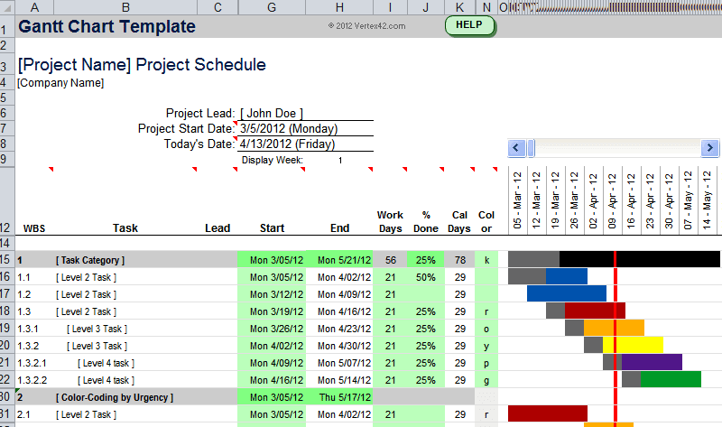
I just found out a reporting structure mockup I have prepared in Excel once upon a time:

A bit blurry but explains the purpose

By the way, did you see our Automatic Organization Chart Generator?

This is an Excel template that lets you create organization charts from Excel lists with a click of a button. It can be useful for small business owners and Human Resources departments.

These type of charts are directly related to Excel as most of the companies already keep their data in spreadsheets. But I also know people who even build their website mockups in Excel (with links to other sections, placement of buttons, sliders etc.).

Sometimes you may need your excel files to be updated automatically from a live data source. For example, if you are making a stock market analysis and want the latest data of some stock prices at NYSE, you can connect your Excel file to a data feed and let it take the latest info automatically (unless you want to input them one by one!)

As this is a comprehensive topic I will leave it for another post. But here is a few things you can fetch into excel:

Stock prices
Match results of soccer, NBA, NFL or any sports games (from live score sites)
Fx rates
Real-time flight data of airports
Any info in a shared database (whether it is your company intranet or public)

This topic is getting more and more important as most data is kept on cloud systems. We don’t download info bits to our computers as we used to do in the past. So, Microsoft is working hard to improve the web integration of Excel.

Recommended Reading: Can Excel Extract Data From Website?

Yes, it is not the best idea to use Excel as a database. Because it is not designed for this purpose. Queries will take a long time especially when data gets bigger. It can be unreliable sometimes and not very secure. It is all accepted. However, we are not always after a complete set of the database systems and it can serve us as a mini-warehouse for our little data.

For example, if you keep records of your invoice data and want to make some sales analysis, it can be a good starting point. If later, you want to see more details, want to record more breakdowns you will need to move to a “real database”. It can be Access, SQL or anything. Just keep an eye on your Excel file because it has a maximum of 1 million rows.

Some of you may say “hey, it is more than enough, isn’t it?”

Generally yes. But you cannot believe how data increase in size when you want to see details. I remember when I was working as an analyst in a game development company, we were holding records of 1+ billion rows of data.

Precisely because of that, we have built some of our Excel templates (which is the favorite feature of all the users) with a database section. You may check our Invoice Generators and see how invoice recording would be super easy in Excel!

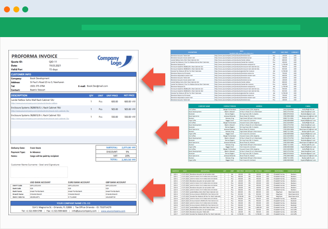
Someka Invoice Generators in Excel

Conclusion

As the internet gets more available for everybody people started to use collaboration platforms more than before. In this aspect, online spreadsheet applications, like Google Sheets, increase in popularity and stands as a competitor to Microsoft’s Excel. Other free alternatives like open office or libre office are also popular. But if you need the advanced functionalities of Excel there is still no substitute.

Microsoft is improving the software actively. PowerPivot, Power BI, and Excel Online are all brand new features they developed recently. We will wait and see how things evolve in the following years. (investintech.com has made interviews with Excel experts about the future of Excel)

I tried to cover most of the things that can be done with Excel. If I have missed anything or if you find any errors, let me know by commenting down or sending an email.

Also, don’t forget to check our Excel Templates Collection. You may find something useful for yourself:

Excel Templates and Spreadsheets – Someka

Источник

На чтение 16 мин. Просмотров 14.6k.

Malcolm Gladwell

Мечтатель начинает с чистого листа бумаги и переосмысливает мир

Эта статья содержит полное руководство по использованию Excel
VBA Worksheet в Excel VBA. Если вы хотите узнать, как что-то сделать быстро, ознакомьтесь с кратким руководством к рабочему листу VBA ниже.

Если вы новичок в VBA, то эта статья — отличное место для начала. Мне нравится разбивать вещи на простые термины и объяснять их на простом языке.

Вы можете прочитать статью от начала до конца, так как она написана в логическом порядке. Или, если предпочитаете, вы можете использовать оглавление ниже и перейти непосредственно к теме по вашему выбору.

Содержание

Краткое руководство к рабочему листу VBA
Вступление
Доступ к рабочему листу
Использование индекса для доступа к рабочему листу
Использование кодового имени рабочего листа
Активный лист
Объявление объекта листа
Доступ к рабочему листу в двух словах
Добавить рабочий лист
Удалить рабочий лист
Цикл по рабочим листам
Использование коллекции листов
Заключение

Краткое руководство к рабочему листу VBA

В следующей таблице приведен краткий обзор различных методов
Worksheet .

Примечание. Я использую Worksheet в таблице ниже, не указывая рабочую книгу, т.е. Worksheets, а не ThisWorkbook.Worksheets, wk.Worksheets и т.д. Это сделано для того, чтобы примеры были понятными и удобными для чтения. Вы должны всегда указывать рабочую книгу при использовании Worksheets . В противном случае активная рабочая книга будет использоваться по умолчанию.

Задача	Исполнение
Доступ к рабочему листу по имени	Worksheets(«Лист1»)
Доступ к рабочему листу по позиции слева	Worksheets(2) Worksheets(4)
Получите доступ к самому левому рабочему листу	Worksheets(1)
Получите доступ к самому правому листу	Worksheets(Worksheets.Count)
Доступ с использованием кодового имени листа (только текущая книга)	Смотри раздел статьи Использование кодового имени
Доступ по кодовому имени рабочего листа (другая рабочая книга)	Смотри раздел статьи Использование кодового имени
Доступ к активному листу	ActiveSheet
Объявить переменную листа	Dim sh As Worksheet
Назначить переменную листа	Set sh = Worksheets(«Лист1»)
Добавить лист	Worksheets.Add
Добавить рабочий лист и назначить переменную	Worksheets.Add Before:= Worksheets(1)
Добавить лист в первую позицию (слева)	Set sh =Worksheets.Add
Добавить лист в последнюю позицию (справа)	Worksheets.Add after:=Worksheets(Worksheets.Count)
Добавить несколько листов	Worksheets.Add Count:=3
Активировать рабочий лист	sh.Activate
Копировать лист	sh.Copy
Копировать после листа	sh1.Copy After:=Sh2
Скопировать перед листом	sh1.Copy Before:=Sh2
Удалить рабочий лист	sh.Delete
Удалить рабочий лист без предупреждения	Application.DisplayAlerts = False sh.Delete Application.DisplayAlerts = True
Изменить имя листа	sh.Name = «Data»
Показать/скрыть лист	sh.Visible = xlSheetHidden sh.Visible = xlSheetVisible sh.Name = «Data»
Перебрать все листы (For)	Dim i As Long For i = 1 To Worksheets.Count Debug.Print Worksheets(i).Name Next i
Перебрать все листы (For Each)	Dim sh As Worksheet For Each sh In Worksheets Debug.Print sh.Name Next

Вступление

Три наиболее важных элемента VBA — это Рабочая книга, Рабочий лист и Ячейки. Из всего кода, который вы пишете, 90% будут включать один или все из них.

Наиболее распространенное использование Worksheet в VBA для доступа к его ячейкам. Вы можете использовать его для защиты, скрытия, добавления, перемещения или копирования листа.

Тем не менее, вы будете в основном использовать его для выполнения некоторых действий с одной или несколькими ячейками на листе.

Использование Worksheets более простое, чем использование рабочих книг. С книгами вам может потребоваться открыть их, найти, в какой папке они находятся, проверить, используются ли они, и так далее. С рабочим листом он либо существует в рабочей книге, либо его нет.

Доступ к рабочему листу

В VBA каждая рабочая книга имеет коллекцию рабочих листов. В этой коллекции есть запись для каждого рабочего листа. Эта коллекция называется просто Worksheets и используется очень похоже на коллекцию Workbooks. Чтобы получить доступ к рабочему листу, достаточно указать имя.

Приведенный ниже код записывает «Привет Мир» в ячейках A1 на листах: Лист1, Лист2 и Лист3 текущей рабочей книги.

Sub ZapisVYacheiku1()

    ' Запись в ячейку А1 в листе 1, листе 2 и листе 3
    ThisWorkbook.Worksheets("Лист1").Range("A1") = "Привет Мир"
    ThisWorkbook.Worksheets("Лист2").Range("A1") = "Привет Мир"
    ThisWorkbook.Worksheets("Лист3").Range("A1") = "Привет Мир"

End Sub

Коллекция Worksheets всегда принадлежит книге. Если мы не
указываем рабочую книгу, то активная рабочая книга используется по умолчанию.

Sub ZapisVYacheiku1()

    ' Worksheets относятся к рабочим листам в активной рабочей книге.
    Worksheets("Лист1").Range("A1") = "Привет Мир"
    Worksheets("Лист2").Range("A1") = "Привет Мир"
    Worksheets("Лист3").Range("A1") = "Привет Мир"

End Sub

Скрыть рабочий лист

В следующих примерах показано, как скрыть и показать лист.

ThisWorkbook.Worksheets("Лист1").Visible = xlSheetHidden

ThisWorkbook.Worksheets("Лист1").Visible = xlSheetVisible

Если вы хотите запретить пользователю доступ к рабочему
листу, вы можете сделать его «очень скрытым». Это означает, что это может быть
сделано видимым только кодом.

' Скрыть от доступа пользователя
ThisWorkbook.Worksheets("Лист1").Visible = xlVeryHidden

' Это единственный способ сделать лист xlVeryHidden видимым
ThisWorkbook.Worksheets("Лист1").Visible = xlSheetVisible

Защитить рабочий лист

Другой пример использования Worksheet — когда вы хотите защитить его.

ThisWorkbook.Worksheets("Лист1").Protect Password:="Мойпароль"

ThisWorkbook.Worksheets("Лист1").Unprotect Password:="Мойпароль"

Индекс вне диапазона

При использовании Worksheets вы можете получить сообщение об
ошибке:

Run-time Error 9 Subscript out of Range

Это означает, что вы пытались получить доступ к рабочему листу, который не существует. Это может произойти по следующим причинам:

Имя Worksheet , присвоенное рабочим листам, написано неправильно.
Название листа изменилось.
Рабочий лист был удален.
Индекс был большим, например Вы использовали рабочие листы (5), но есть только четыре рабочих листа
Используется неправильная рабочая книга, например Workbooks(«book1.xlsx»).Worksheets(«Лист1») вместо
Workbooks(«book3.xlsx»).Worksheets («Лист1»).

Если у вас остались проблемы, используйте один из циклов из раздела «Циклы по рабочим листам», чтобы напечатать имена всех рабочих листов коллекции.

Использование индекса для доступа к рабочему листу

До сих пор мы использовали имя листа для доступа к листу.
Указатель относится к положению вкладки листа в рабочей книге. Поскольку
положение может быть легко изменено пользователем, не рекомендуется
использовать это.

В следующем коде показаны примеры использования индекса.

' Использование этого кода является плохой идеей, так как
' позиции листа все время меняются
Sub IspIndList()

    With ThisWorkbook
        ' Самый левый лист
        Debug.Print .Worksheets(1).Name
        ' Третий лист слева
        Debug.Print .Worksheets(3).Name
        ' Самый правый лист
        Debug.Print .Worksheets(.Worksheets.Count).Name
    End With

End Sub

В приведенном выше примере я использовал Debug.Print для печати в Immediate Window. Для просмотра этого окна выберите «Вид» -> «Immediate Window » (Ctrl + G).

Использование кодового имени рабочего листа

Лучший способ получить доступ к рабочему листу —
использовать кодовое имя. Каждый лист имеет имя листа и кодовое имя. Имя листа
— это имя, которое отображается на вкладке листа в Excel.

Изменение имени листа не приводит к изменению кодового имени, что означает, что ссылка на лист по кодовому имени — отличная идея.

Если вы посмотрите в окне свойств VBE, вы увидите оба имени.
На рисунке вы можете видеть, что кодовое имя — это имя вне скобок, а имя листа
— в скобках.

Вы можете изменить как имя листа, так и кодовое имя в окне
свойств листа (см. Изображение ниже).

Width

Если ваш код ссылается на кодовое имя, то пользователь может
изменить имя листа, и это не повлияет на ваш код. В приведенном ниже примере мы
ссылаемся на рабочий лист напрямую, используя кодовое имя.

Sub IspKodImya2()

    ' Используя кодовое имя листа
    Debug.Print CodeName.Name
    CodeName.Range("A1") = 45
    CodeName.Visible = True

End Sub

Это делает код легким для чтения и безопасным от изменения
пользователем имени листа.

Кодовое имя в других книгах

Есть один недостаток использования кодового имени. Он относится только к рабочим листам в рабочей книге, которая содержит код, т.е. ThisWorkbook.

Однако мы можем использовать простую функцию, чтобы найти
кодовое имя листа в другой книге.

Sub ИспЛист()

    Dim sh As Worksheet
    ' Получить рабочий лист под кодовым именем
    Set sh = SheetFromCodeName("CodeName", ThisWorkbook)
    ' Используйте рабочий лист
    Debug.Print sh.Name

End Sub

' Эта функция получает объект листа из кодового имени
Public Function SheetFromCodeName(Name As String, bk As Workbook) As Worksheet

    Dim sh As Worksheet
    For Each sh In bk.Worksheets
        If sh.CodeName = Name Then
           Set SheetFromCodeName = sh
           Exit For
        End If
    Next sh

End Function

Использование приведенного выше кода означает, что если
пользователь изменит имя рабочего листа, то на ваш код это не повлияет.

Существует другой способ получения имени листа внешней
рабочей книги с использованием кодового имени. Вы можете использовать элемент
VBProject этой Рабочей книги.

Вы можете увидеть, как это сделать, в примере ниже. Я включил это, как дополнительную информацию, я бы рекомендовал использовать метод из предыдущего примера, а не этот.

Public Function SheetFromCodeName2(codeName As String _
                             , bk As Workbook) As Worksheet

    ' Получить имя листа из CodeName, используя VBProject
    Dim sheetName As String
    sheetName = bk.VBProject.VBComponents(codeName).Properties("Name")

    ' Используйте имя листа, чтобы получить объект листа
    Set SheetFromCodeName2 = bk.Worksheets(sheetName)

End Function

Резюме кодового имени

Ниже приведено краткое описание использования кодового имени:

Кодовое имя рабочего листа может быть
использовано непосредственно в коде, например. Sheet1.Range
Кодовое имя будет по-прежнему работать, если имя
рабочего листа будет изменено.
Кодовое имя может использоваться только для
листов в той же книге, что и код.
Везде, где вы видите ThisWorkbook.Worksheets
(«имя листа»), вы можете заменить его кодовым именем рабочего листа.
Вы можете использовать функцию SheetFromCodeName
сверху, чтобы получить кодовое имя рабочих листов в других рабочих книгах.

Активный лист

Объект ActiveSheet ссылается на рабочий лист, который в данный момент активен. Вы должны использовать ActiveSheet только в том случае, если у вас есть особая необходимость ссылаться на активный лист.

В противном случае вы должны указать рабочий лист, который
вы используете.

Если вы используете метод листа, такой как Range, и не
упоминаете лист, он по умолчанию будет использовать активный лист.

' Написать в ячейку A1 в активном листе
ActiveSheet.Range("A1") = 99

' Активный лист используется по умолчанию, если лист не используется
Range("A1") = 99

Объявление объекта листа

Объявление объекта листа полезно для того, чтобы сделать ваш
код более понятным и легким для чтения.

В следующем примере показан код для обновления диапазонов
ячеек. Первый Sub не объявляет объект листа. Вторая подпрограмма объявляет
объект листа, и поэтому код намного понятнее.

Sub NeObyavObektList()

    Debug.Print ThisWorkbook.Worksheets("Лист1").Name
    ThisWorkbook.Worksheets("Лист1").Range("A1") = 6
    ThisWorkbook.Worksheets("Лист1").Range("B2:B9").Font.Italic = True
    ThisWorkbook.Worksheets("Лист1").Range("B2:B9").Interior.Color = rgbRed

End Sub

Sub ObyavObektList()

    Dim sht As Worksheet
    Set sht = ThisWorkbook.Worksheets("Лист1")

    sht.Range("A1") = 6
    sht.Range("B2:B9").Font.Italic = True
    sht.Range("B2:B9").Interior.Color = rgbRed

End Sub

Вы также можете использовать ключевое слово With с объектом
листа, как показано в следующем примере.

Sub ObyavObektListWith()

    Dim sht As Worksheet
    Set sht = ThisWorkbook.Worksheets("Лист1")

    With sht
        .Range("A1") = 6
        .Range("B2:B9").Font.Italic = True
        .Range("B2:B9").Interior.Color = rgbRed
    End With

End Sub

Доступ к рабочему листу в двух словах

Из-за множества различных способов доступа к рабочему листу вы можете быть сбитыми с толку. Так что в этом разделе я собираюсь разбить его на простые термины.

Если вы хотите использовать тот лист, который активен в данный момент, используйте ActiveSheet.

ActiveSheet.Range("A1") = 55

2. Если лист находится в той же книге, что и код, используйте кодовое имя.

3. Если рабочая таблица находится в другой рабочей книге, сначала получите рабочую книгу, а затем получите рабочую таблицу.

' Получить рабочую книгу
Dim wk As Workbook
Set wk = Workbooks.Open("C:ДокументыСчета.xlsx", ReadOnly:=True)
' Затем получите лист
Dim sh As Worksheet
Set sh = wk.Worksheets("Лист1")

Если вы хотите защитить пользователя от изменения имени листа, используйте функцию SheetFromCodeName из раздела «Имя кода».

' Получить рабочую книгу
Dim wk As Workbook
Set wk = Workbooks.Open("C:ДокументыСчета.xlsx", ReadOnly:=True)

' Затем получите лист
Dim sh As Worksheet
Set sh = SheetFromCodeName("sheetcodename",wk)

Добавить рабочий лист

Примеры в этом разделе показывают, как добавить новую
рабочую таблицу в рабочую книгу. Если вы не предоставите никаких аргументов для
функции Add, то новый
рабочий лист будет помещен перед активным рабочим листом.

Когда вы добавляете рабочий лист, он создается с именем по умолчанию, например «Лист4». Если вы хотите изменить имя, вы можете легко сделать это, используя свойство Name.

В следующем примере добавляется новый рабочий лист и изменяется имя на «Счета». Если лист с именем «Счета» уже существует, вы получите сообщение об ошибке.

Sub DobavitList()

    Dim sht As Worksheet

    ' Добавляет новый лист перед активным листом
    Set sht = ThisWorkbook.Worksheets.Add
    ' Установите название листа
    sht.Name = "Счета"

    ' Добавляет 3 новых листа перед активным листом
    ThisWorkbook.Worksheets.Add Count:=3

End Sub

В предыдущем примере вы добавляете листы по отношению к
активному листу. Вы также можете указать точную позицию для размещения листа.

Для этого вам нужно указать, какой лист новый лист должен
быть вставлен до или после. Следующий код показывает вам, как это сделать.

Sub DobavitListPervPosl()

    Dim shtNew As Worksheet
    Dim shtFirst As Worksheet, shtLast As Worksheet

    With ThisWorkbook

        Set shtFirst = .Worksheets(1)
        Set shtLast = .Worksheets(.Worksheets.Count)

        ' Добавляет новый лист на первую позицию в книге
        Set shtNew = Worksheets.Add(Before:=shtFirst)
        shtNew.Name = "FirstSheet"

        ' Добавляет новый лист к последней позиции в книге
        Set shtNew = Worksheets.Add(After:=shtLast)
        shtNew.Name = "LastSheet"

    End With

End Sub

Удалить рабочий лист

Чтобы удалить лист, просто вызовите Delete.

Dim sh As Worksheet
Set sh = ThisWorkbook.Worksheets("Лист12")
sh.Delete

Excel отобразит предупреждающее сообщение при удалении листа. Если вы хотите скрыть это сообщение, вы можете использовать код ниже:

Application.DisplayAlerts = False
sh.Delete
Application.DisplayAlerts = True

Есть два аспекта, которые нужно учитывать при удалении таблиц.

Если вы попытаетесь получить доступ к рабочему листу после
его удаления, вы получите ошибку «Subscript out of Range», которую мы видели в
разделе «Доступ к рабочему листу».

Dim sh As Worksheet
Set sh = ThisWorkbook.Worksheets("Лист2")
sh.Delete

' Эта строка выдаст «Subscript out of Range», так как «Лист2» не существует
Set sh = ThisWorkbook.Worksheets("Лист2")

Вторая проблема — когда вы назначаете переменную листа. Если вы попытаетесь использовать эту переменную после удаления листа, вы получите ошибку автоматизации, подобную этой:

Run-Time error -21147221080 (800401a8′) Automation Error

Если вы используете кодовое имя рабочего листа, а не
переменную, это приведет к сбою Excel,
а не к ошибке автоматизации.

В следующем примере показано, как происходят ошибки автоматизации.

sh.Delete

' Эта строка выдаст ошибку автоматизации
Debug.Assert sh.Name

Если вы назначите переменную Worksheet действительному рабочему листу, он будет работать нормально.

sh.Delete

' Назначить sh на другой лист
Set sh = Worksheets("Лист3")

' Эта строка будет работать нормально
Debug.Assert sh.Name

Цикл по рабочим листам

Элемент «Worksheets» — это набор рабочих листов, принадлежащих рабочей книге. Вы можете просмотреть каждый лист в коллекции рабочих листов, используя циклы «For Each» или «For».

В следующем примере используется цикл For Each.

Sub CiklForEach()

    ' Записывает «Привет Мир» в ячейку A1 для каждого листа
    Dim sht As Worksheet
    For Each sht In ThisWorkbook.Worksheets
         sht.Range("A1") = "Привет Мир"
    Next sht 

End Sub

В следующем примере используется стандартный цикл For.

Sub CiklFor()
    
    ' Записывает «Привет Мир» в ячейку A1 для каждого листа
    Dim i As Long
    For i = 1 To ThisWorkbook.Worksheets.Count
         ThisWorkbook.Worksheets(i).Range("A1") = "Привет Мир"
    Next sht

End Sub

Вы видели, как получить доступ ко всем открытым рабочим книгам и как получить доступ ко всем рабочим листам в ThisWorkbook. Давайте сделаем еще один шаг вперед — узнаем, как получить доступ ко всем рабочим листам во всех открытых рабочих книгах.

Примечание. Если вы используете код, подобный этому, для записи на листы, то сначала сделайте резервную копию всего, так как в итоге вы можете записать неверные данные на все листы.

Sub NazvVsehStr()

    ' Печатает рабочую книгу и названия листов для
    ' всех листов в открытых рабочих книгах
    Dim wrk As Workbook
    Dim sht As Worksheet
    For Each wrk In Workbooks
        For Each sht In wrk.Worksheets
            Debug.Print wrk.Name + ":" + sht.Name
        Next sht
    Next wrk

End Sub

Использование коллекции листов

Рабочая книга имеет еще одну коллекцию, похожую на Worksheets под названием Sheets. Это иногда путает пользователей. Чтобы понять, в первую очередь, вам нужно знать о типе листа, который является диаграммой.

В Excel есть возможность создать лист, который является диаграммой. Для этого нужно:

Создать диаграмму на любом листе.
Щелкнуть правой кнопкой мыши на графике и выбрать «Переместить».
Выбрать первый вариант «Новый лист» и нажмите «ОК».

Теперь у вас есть рабочая книга, в которой есть типовые листы и лист-диаграмма.

Коллекция «Worksheets » относится ко всем рабочим листам в рабочей книге. Не включает в себя листы типа диаграммы.
Коллекция Sheets относится ко всем листам, принадлежащим книге, включая листы типовой диаграммы.

Ниже приведены два примера кода. Первый проходит через все
листы в рабочей книге и печатает название листа и тип листа. Второй пример
делает то же самое с коллекцией Worksheets.

Чтобы опробовать эти примеры, вы должны сначала добавить лист-диаграмму в свою книгу, чтобы увидеть разницу.

Sub KollSheets()

    Dim sht As Variant
    ' Показать название и тип каждого листа
    For Each sht In ThisWorkbook.Sheets
        Debug.Print sht.Name & " is type " & TypeName(sht)
    Next sht

End Sub

Sub KollWorkSheets()

    Dim sht As Variant
    ' Показать название и тип каждого листа
    For Each sht In ThisWorkbook.Worksheets
        Debug.Print sht.Name & " is type " & TypeName(sht)
    Next sht

End Sub

Если у вас нет листов диаграмм, то использование коллекции Sheets — то же самое, что использование коллекции WorkSheets.

Заключение

На этом мы завершаем статью о Worksheet VBA. Я надеюсь, что было полезным.

Три наиболее важных элемента Excel VBA — это рабочие книги, рабочие таблицы, диапазоны и ячейки.

Эти элементы будут использоваться практически во всем, что вы делаете. Понимание их сделает вашу жизнь намного проще и сделает изучение VBA увлекательнее.

Источник

15 Most Common Excel Functions You Must Know + How to Use Them

Microsoft Excel is one of the most well-known computer applications. It has changed the way people and companies work with data.

Thus, learning Excel can help with both your career and your personal needs.

Excel runs using functions and there are roughly 500 of them! These range from basic arithmetic to complex statistics.

Most Excel users will only ever use about 100 of these functions

If you’re a new Excel user, this sheer quantity can be quite daunting.

So we are here to help you! 🤝

We have rounded up 15 of the most common and useful Excel functions that you need to learn. We also prepared a practice workbook for you to follow along with the examples. Download it here.

Let’s get started!

What are Excel functions?

Excel is used to calculate and manipulate numbers and text. To do this, you use formulas!

Formulas are expressions that tell Excel what you want to do with the data. They begin with the equal symbol (=) followed by a combination of operators and functions.

What are operators?

These are symbols that specify the type of calculation you want to perform on the elements of a formula.

For example, to add two numbers, you can type “=1+1” into a cell. Once you hit Enter, Excel will run the formula and return the result which is 2.

Here are some examples of common operators:

An arithmetic calculation return a number, comparisons return a Boolean or logical value i.e. TRUE or FALSE

Excel automatically treats cell contents that start with (=) as formulas. This also applies when you begin a cell with the plus (+) or minus (-) symbols.

You can bypass this by adding a leading apostrophe (‘). This is how you can show formulas as text like in the table above.

Order of operation and using parentheses in Excel formulas

Generally, Excel follows PEMDAS when calculating formulas. PEMDAS means parentheses first, then exponents, then multiplication and division, then addition and subtraction.

Adding parentheses changes how a formula calculates

What are functions?

These are predefined processes in Excel. Each function in Excel has a unique name and specific input(s). The function takes these inputs and performs the corresponding calculation.

The inputs or arguments of an Excel function are always enclosed in parentheses.

For example, this is the syntax for the MAX function:

=MAX(number1, [number2], …)

The list of numbers where you want to find the maximum value is placed inside the parentheses.

MAX returns the maximum value from a group of numbers, the function MIN does the same for the minimum value

Using a cell or a range as input

As you learn more about Excel, you’ll find that Excel formulas rarely consist of individual numbers only like in the formula “=1+1”.

Often, you need to reference a cell or a range(group of cells) as the input of your Excel function

Thus, referencing cells is important in Excel and you can learn more by clicking here.

Alright! You’ve just learned how a function in Excel works.

Let’s dive right into the list! 🤿

We will start with basic Excel functions and then move on to more advanced functions.

Basic Math Functions (Beginner Level ★☆☆)

1. SUM

This is the first function in Excel that most new users need. As the name implies, the SUM function adds up all the values in a specified group of cells or range.

Syntax: =SUM(number1, [number2], …)

Try it out in the practice workbook.

If you want to get the total quiz score for each student, you can use the SUM function. In this case, the input range will be all four quiz scores for each student.

1. Type this formula into cell F2:

=SUM(B2:E2)

You can also type “=SUM(B2,C2,D2,E2)” but “=SUM(B2:E2)” is much simpler.

You can also drag the input selection(blue box) over to your desired range

2. Press Enter. Excel then evaluates the formula and the cell returns the number for the total which is 360.

3. Copy this for the rest of the students or drag down the fill handle.

The fill handle is the small green square at bottom right of the cell

Notice that the SUM function ignores the cells containing text. (“X” meaning the student was unable to take the quiz)

Most of the basic math functions in Excel ignore non-numeric values such as text, date, and time.

2. COUNT

Next up is the COUNT function. It returns the number of cells containing numeric values within the input range.

Syntax: =COUNT(value1, [value2], …)

1. To get the number of quizzes taken by each student, use this formula in cell G2:

=COUNT(B2:E2)

2. Hit Enter and fill in the rows below.

If you would like to include non-numeric values in the count, you can use the COUNTA function. To count the number of blank cells, you can use the COUNTBLANK function.

Learn more about the COUNT function and its variants here.

3. AVERAGE

The average of a list of numbers is just the total divided by how many numbers there are in that list.

This is easy enough to calculate the quiz scores. You already have the SUM and the COUNT of quizzes for each student.

But, it gets even easier using the AVERAGE function in Excel.

Syntax: =AVERAGE (value1, [value2], …)

1. Type this into cell H2:

=AVERAGE(B2:E2)

2. Hit Enter and fill in the rows below.

Use Cell Formatting to change the number of decimals displayed

You can double-check the results using the SUM and COUNT functions earlier.

Logical Functions (Intermediate Level – ★★☆)

Let’s raise the difficulty level a little bit.

A logical function in Excel allows you to make comparisons and use the results to change how a formula calculates.

4. IF

The IF function is a very popular function in Excel and it is actually quite easy to learn.

Syntax: =IF(logical_test, value_if_true, [value_if_false])

This function checks if a logical test is either TRUE or FALSE. It then returns the specified value based on the result.

Using the average score of each student, try to assign PASS or FAIL grades. Assume that the passing score for this class is 60.

1. Begin the formula in cell C2 with “=IF(“

The logical_test is to check if the average score in Column B is greater than or equal to (>=) the passing score of 60.

2. So, the formula becomes:

=IF(B2>=60,

If the comparison returns TRUE, then the formula should return the text “PASS”. Thus, the value_if_true argument should be “PASS”.

And if it returns FALSE, then the value_if_false argument should be “FAIL”.

3. Thus, the formula becomes:

=IF(B2>=60,”PASS”,”FAIL”)

4. Hit Enter and fill in the rows below.

Luckily everyone in this class has passed

What if you needed to assign grades according to a scale instead of just “PASS” and “FAIL”?

For that, you have to use multiple criteria or logical tests. While this is possible using nested IF functions, it can get messy very quickly. Instead, you can use the IFS function.

5. IFS function

The IFS function was introduced in Excel 2016 to replace nested IF functions.

This function works by evaluating the first logical test or criteria. It returns the corresponding value if it is TRUE. But if it is FALSE, the function proceeds to evaluate the second criteria, and so on.

📖 In other words, the IFS function outputs the value that corresponds to the first specified criteria that is true.

Syntax: =IFS(logical_test1, value_if_true1, [logical_test2], [value_if_true2],..)

Use the grading table on the right as reference

1. First, the formula should check if the average score (column B) is above or equal to 90. If yes, it should return “A”.

=IFS(B2>=90,”A”,

2. If not, it should then check if the average score is greater than or equal to 80. If yes, it should return “B”. If you do this up to grade D, the formula becomes:

=IFS(B2>=90,”A”,B2>=80,”B”,B2>=70,”C”,B2>=60,”D”,

3. For the last grade “F”, put “TRUE” for the logical test.

The IFS function will only evaluate the last specified criteria if all of the previous logical values were FALSE. Thus, you can set the last criteria to always be TRUE thus making it a “catch all” statement.

The final formula is then:

=IFS(B2>=90,”A”,B2>=80,”B”,B2>=70,”C”,B2>=60,”D”,TRUE,”F”)

PRO-TIP:

You can use absolute cell references and a reference table when working with long formulas.

That way, you don’t have to revisit all of the arguments in the formula if you need to change some values.

For example, using the table and formula shown below, you can easily change the grading scale in use.

=IFS(B2>=$H$2,$F$2,B2>=$H$3,$F$3,B2>
=$H$4,$F$4,B2>=$H$5,$F$5,TRUE,$F$6)

The dollar sign ($) in a formula denotes an absolute cell reference, ex: $F$2

Text Functions (Intermediate Level – ★★☆)

In this next section, you will see how Excel can also be used to manipulate text.

In the “Class List” worksheet of the practice workbook, the full name of each student is listed in Column A. Your goal is to rearrange these from “first name last name” to “last name_first name” in Column F.

The finished table will let users sort using both first and last name

To do this, you first have to extract the first name and the last name from Column A.

6. FIND

The names are separated by a space character ” “. So, you have to identify the position of the space within each text string in Column A.

The FIND function in Excel returns the number or position of a specified character or substring within another text string.

Syntax: =FIND(find_text, within_text, [start_num])

To get the position of the space ” “, type this formula:

=FIND(” “,A2)

You will use these results to extract the first name later

Next, take a look at the LEN function.

7. LEN

This function returns the number of characters in a text string.

Syntax: =LEN(text)

To get the number of characters in each student’s name:

=LEN(A2)

You will use the LEN results to extract the last name later

Now you can move on to extracting the first and last name using the MID function in Excel.

8. MID

This function extracts a given number of characters from the middle of a text string.

Syntax: = MID(text, start_num, num_chars)

It is one of three text functions that are used to extract text. The other two are LEFT and RIGHT which extract text from the start and end of a text string respectively.

The first name starts at the very first character of the text string. So, you extract starting from position 1. Then the length of the first name is given by the position of the space character minus 1.

So, the formula to extract the first name or first word from a text string is:

=MID(A2,1,B2-1)

Or, you can express it directly using the FIND formula earlier.

=MID(A2,1,FIND(” “,A2)-1)

This formula works for any text string you need to grab the first word from

For the last name, you can extract it starting from the position of the space character plus 1. Its length is just the length of the entire text string minus the position of the space character.

=MID(A2,B2+1,C2-B2)

Or, using the FIND and LEN formulas earlier:

=MID(A2,FIND(” “,A2)+1,LEN(A2)-FIND(” “,A2))

The space character's position number raised by 1 gives the starting position of the last name

Now you can combine the last name and the first name in the desired order using the CONCAT function.

9. CONCAT

Like IFS, CONCAT is another newly introduced function in Excel 2016. It replaced the old CONCATENATE function.

Syntax: =CONCAT(text1, [text2],…)

Combine the last name and the first name with a comma and space character “, ” in between.

=CONCAT(E2,”, “,D2)

CONCAT also converts input numbers to text

PRO-TIP:

In the above example, you used helper columns for FIND, LEN, and MID to help build the final formula and visualize how it works.

In real-world applications, you can use a single long formula to get the results like this:

=CONCAT(MID(A2,FIND(” “,A2)+1,LEN(A2)
-FIND(” “,A2)),”, “,MID(A2,1,FIND(” “,A2)-1))

Helper columns are useful in building and testing long formulas

Lookup and Reference Functions (Advanced Level – ★★★)

In this final section, we will focus on functions that allow you to look for specific data points and refer to them.

Take a look at the “Schedule” worksheet.

You will find the schedule and seating plan for the next four quizzes

10. COLUMN

The COLUMN function in Excel returns the column number of a given cell.

Syntax: =COLUMN([reference])

Let’s try to assign specific dates for each quiz. For example, you may want the quizzes to be held every Monday. This means that the first quiz date should be offset by 1 week or 7 days for each succeeding quiz date.

You can use the column number to multiply the 7 days offset for each week like this:

=$B$2+(COLUMN()-2)*7

The start date, Oct 3, is highlighted in green and its column number, 2, is subtracted from the formula

Two (2) is subtracted from the column number so that the sequence starts at 1.

You can also get this result using the much simpler “=B2+7” since you are only adding a fixed number of days to each date. 🤔

But, using the COLUMN function, you can create complex patterns.

Take this pattern for example:

The quizzes are still held every Monday. But every third week, they are held on Wednesday instead.

Here is the formula for this pattern:

=$B$2+(COLUMN()-2)*7+IF(MOD(COLUMN()-1,3)=0,2,0)

The formula is a bit long so here is a breakdown of how it works

The MOD function in Excel returns the remainder after a number is divided by a given divisor. It’s part of the Math & Trig group of functions.

This group includes other fun functions such as ABS which returns the absolute value of a number and ROUND which rounds a number to a specified number of digits.

Learn more about the function groups towards the end of this article!

Kasper Langmann, Microsoft Office Specialist

11. ROW

Next, take a look at the ROW function. It works exactly like COLUMN but it returns the row number instead.

Syntax: =ROW([reference])

In this next example, you will assign the seating plans. You can try different seating arrangements using the ROW function.

Assume R1C1 is the seat closest to the teacher’s desk.

1. You can have the students seated one seat after another and in two columns:

=CONCAT(“R”,MOD(ROW()-6,3)*2+1,”C”,INT((ROW()-6)/3)*2+1)

The INT function in Excel rounds a number down to the nearest integer

2. Or they can sit in rows of 3 and columns of 2

=CONCAT(“R”,MOD(ROW()-6,2)*2+1,”C”,INT((ROW()-6)/2)*2+1)

You can modify the values in the formula to change the seating pattern

3. You can also sit them in the farthest rows:

=CONCAT(“R”,MOD(ROW()-6,2)*4+1,”C”,INT((ROW()-6)/2)*2+1)

In this seating plan, students have the most distance from the front and back

4. Or in the farthest columns:

=CONCAT(“R”,MOD(ROW()-6,3)*2+1,”C”,INT((ROW()-6)/3)*4+1)

In this seating plan, students have the most distance from the sides

Manually creating seating patterns for small sets like this one is easy. But a formula like those shown above definitely helps especially for larger sets like 50, 100, or even more.

The COLUMN and ROW functions are rarely used on their own. Like IF and IFS, you use them with other functions to change how the formula is calculated.

12. MATCH

Now, open up the “Lookup” worksheet.

In the next few examples, you will create a search feature that allows students to look up their names. They can then see their scores from past quizzes and their assigned seats for the next quizzes.

To start, you will use the MATCH function. It searches for a specified item within a given range of cells. It then returns the relative position of the first match.

Syntax: =MATCH(lookup_value, lookup_array, [match_type])

The lookup_value is the item you want to search for. So, set this to cell B2.
The lookup_array is the range or table array where you want to search. Use F2:F7 from the “Class List” worksheet.
For the match_type, set this to zero so that the function searches for an exact match. (Learn more about MATCH and the different match types in this article)

The formula then becomes:

=MATCH(B2,’Class List’!F2:F7,0)

Students can now search for their names and the function returns the relative position in the Class List table

However, it only works correctly if the name is entered exactly as it is written in Column F of the Class List.

To fix this, you can use the asterisk “*” wildcard character so that searching for either first or last name works.

You can also enclose the formula in an IFNA function. This way, if the formula cannot find the given name in the table, it will return a phrase like “No result found”.

You will later use the resulting Row to retrieve the first and last name

13. INDEX

The INDEX function retrieves a value from a given table array based on the provided row and column numbers.

Syntax: =INDEX (array, row_num, [col_num])

Similar to the MATCH example, you need to specify where the range or array lookup is.

Use D2:E7 from Class List as the table array

For row_num, you can use the earlier MATCH result at Cell B5. Then for col_num, use 1 for the First Name:

=INDEX(‘Class List’!D2:E7,B5,1)

And set col_num to 2 for the Last Name.

=INDEX(‘Class List’!D2:E7,B5,2)

Just like that, you have a working search 🔍 formula!

This is just a small example of the countless possibilities using the INDEX and MATCH combination. Click here for more examples!

14. VLOOKUP

The VLOOKUP function in Excel works similarly to the INDEX and MATCH combination. It is faster to set up but it is less versatile. VLOOKUP also only works if your lookup array is at the leftmost of the reference table.

Syntax: =VLOOKUP (lookup_value, table_array, col_index_num, [range_lookup])

This time, you will use the First Name result (cell B6) as the lookup_value. Use this and VLOOKUP to retrieve the given student’s scores from the “Quiz Scores” worksheet.

=VLOOKUP($B$6,’Quiz Scores’!$A$2:$E$7,COLUMN(),FALSE)

For the seat assignment, use the Last Name result followed by the asterisk wild character.

=VLOOKUP($B$7&”*”,Schedule!$A$6:$E$11,COLUMN(),FALSE)

15. INDIRECT

The last function that you will be learning about today is also one of the most powerful in Excel.

INDIRECT allows you to specify cell references using text strings.

SYNTAX: =INDIRECT(ref_text, [a1])

For example, instead of typing “=A1”, you can type “=INDIRECT(“A”&1). This means you can dynamically change references.

Let’s take the INDEX & MATCH formula you used to retrieve the Last Name. You can get the same result using this formula:

=INDIRECT(“‘Class List’!”&”E”&(B5+1))

This is a simple example and definitely doesn't do justice to how powerful INDIRECT really is

The INDIRECT function opens up so many possibilities with dynamic references in Excel. I highly this article for an in-depth tutorial on INDIRECT.

That’s it – Now what?

As you have just learned, Excel offers so many different functions to choose from. Luckily, Excel has brought them all together in the Formulas tab.

The functions are categorized into groups such as Math & Trigonometry, Text, & Date and Time

You can look for an Excel function using search keywords or you can also select from the categorical dropdowns.

For example, click on the Financial group to find functions that can help you calculate items like net present value, future value, cumulative interest paid, cumulative principal paid, etc.

NOMINAL returns the annual nominal interest rate

You can also click on More Functions which opens up even more possibilities for advanced Excel formulas.

For example, the Statistical group is useful if you need to calculate a statistical value. This includes functions for maximum value, minimum value, forecast value, gamma function value, etc. You can insert a cumulative distribution function and other useful tools for data analysis.

NORM.DIST can be used either as a cumulative distribution function or as a probability density function

Learn how to use these formulas and more by signing up for my free online Excel course.

We will help you make the most out of your Excel experience! 📈

Other relevant resources

If you enjoyed this article, you can visit my YouTube channel for more in-depth tutorials and other fun stuff!

Did you know that the Flash Fill feature can help speed up your work by automatically filling a repetitive pattern Excel detects from your data? Learn more here.

Thanks for reading! 😄

Kasper Langmann2023-02-23T11:47:15+00:00

Page load link

Источник

In an ideal world, you wouldn’t need to read this tutorial about some of the most important text formulas in Excel.

Unfortunately, we are not in ideal world…

If you work with Excel, you will need to know or learn how to use the LEFT, RIGHT, MID, LEN, FIND and SEARCH functions.

So… fortunately, you have found this tutorial which focuses on some of the most important text functions in Excel.

In this particular Excel tutorial, I explain step-by-step how you can use the LEFT, RIGHT, MID, LEN, FIND and SEARCH functions in Excel.

The following table of contents illustrates, more precisely, the topics we cover in this blog post. You can also use it to skip to the section that interests you the most.

Why You Should Learn How To Use The LEFT, RIGHT, MID, LEN, FIND And SEARCH Functions In Excel
What Are Excel Text Functions
What Is “Text”
Example Of How To Use The LEFT, RIGHT, MID, LEN, FIND And SEARCH Functions In Excel
Step #1: How To Use The LEFT Function In Excel To Determine Whether The First Character In A Cell Is A Number
Step #2: How To Use The IF Function In Excel To Place Each Full Address In A Single Row Of The Excel Worksheet
Step #3: How To Use Filters And Sorting To Delete Blank Rows In Excel Without Loosing Data
Step #4:How To Use The RIGHT Function In Excel To Determine Whether The Last Character In A Cell Is A Space
Step #5: How To Use The LEN Function In Excel To Calculate The Number Of Characters In A Text String
Step #6: How To Use The LEFT Function To Get All The Characters In A Text String Except The Last One
Step #7: How To Use The FIND And SEARCH Functions In Excel
- The FIND And SEARCH Functions In Excel
- How To Apply The FIND Or SEARCH Functions To The Sample Data Set
Step #8: How To Use The LEFT, RIGHT And MID Functions In Excel To Get The Individual Components Of Each Address
- The MID Function In Excel
- How To Use The LEFT, RIGHT And MID Functions To Get The Individual Components Of Each Address
Step #9: How To Use The CONCATENATE Function In Excel To Join All The Components Of An Address In A Single Cell
Conclusion
Books Referenced In This Excel Tutorial

This is a massive amount of content, so let’s begin by understanding…

Why You Should Learn How To Use The LEFT, RIGHT, MID, LEN, FIND And SEARCH Functions In Excel

You may rightly wonder why should you study this comprehensive 11,000+ word tutorial on Excel text formulas to learn how to use some of the most common Excel text functions.

There are several reasons why knowing how to use functions such as LEFT, RIGHT, MID, LEN, FIND and SEARCH is important. But instead of simply listing a bunch of reasons, allow me to ask you a question:

When working with Excel, there are times where you have to use data prepared by other people or companies. Based on your experience, how does this data look like? If you have never worked with data sets prepared by somebody else, please make a guess.

Is it the data set clean, organized, and properly and consistently formatted?
Or is it messy, disorganized, full of clutter and inconsistently formatted?

Let’s face it…

When you receive data prepared by other people or companies, you will need to clean up the data before you can proceed to work with it. In some cases, the data sets will be a complete mess.

And let’s not even talk about the situations where you have to work with several data sets, all prepared by different people who have completely different ideas about how the data should be organized (or disorganized).

When you use data from other sources, it’s usually not ready for analysis. Data scientists spend approximately 80% of their time in the process of gathering and cleaning up data before they can actually begin to analyze it.

The problem of messy data, however, is not exclusive to data analysts. There are many (other) examples. The main point to remember is that data quality is important. Therefore, knowing how to clean up data is essential.

What is the main take-away from the above?

You will need to clean up data. There is no question about it.

Sometimes you may also feel like this:

In order to avoid this type of situation, let’s ask a more relevant question: how will you clean up the data?

Will you do it manually? With the risks of missing errors or introducing new errors? Not to mention the amount of time cleaning up a large data set manually would take or how tedious the work would be…

Or will you automate the data clean-up process as much as possible to make it more streamlined and reliable?

If you are interested in learning how you can start automating the data clean-up process in Excel, keep reading. This Excel tutorial will make you significantly more efficient and productive, and reduce the risk of office violence.

I show you, step-by-step and using a very detailed example, how you can start using the LEFT, RIGHT, MID, LEN, FIND and SEARCH Excel functions now to improve your efficiency and productivity in Excel now.

You may be surprised by what you can do with Excel’s text functions. As explained by John Walkenbach in the Excel 2013 Bible:

(…) some of these formulas perform feats that you may not have thought possible.

Just as an example, quoting Excel Formulas and Functions for Dummies, mastering functions such as LEFT, RIGHT and MID “gives you the power to literally break text apart.”

Does this sound useful?

Then let’s start by understanding…

What Are Excel Text Functions

When you think about Excel, working with text is probably not the first thing that comes to your mind…

That is completely natural. After all, Excel is not a word processor… If you need a word processor, you can use Microsoft Word.

However, you may be surprised by Excel’s capabilities to handle and work with text. This is where Excel text functions come in…

Excel text functions are, as implied by their name, functions you can use to work with text or strings. For these purposes, as explained by John Walkenbach (one of the foremost authorities on Microsoft Excel) in the Excel 2013 Bible, text and string (and sometimes text string) are used interchangeably.

Despite the above, Walkenbach also explains how “many text functions are not limited to text” and, therefore, you can also use some of Excel’s text functions in cells that have numbers.

Excel has several text functions, which you can find by going to the Formulas tab of the Ribbon and clicking on “Text” or using the keyboard shortcut “Alt + M + T”.

What Is “Text”

I’ll ask you a question that may sound a little bit basic but, do you know what is text?

And I don’t mean regular text. I assume that, if you are reading this Excel tutorial, you know what is the usual definition of the word “text”.

The question is actually tricky because, in Excel, some things are slightly different from what you’d usually expect…

In Excel 2013 Formulas, John Walkenbach explains that whenever you type data, “Excel immediately goes to work and determines whether you are entering” one of the following:

A formula.
A number, which includes regular numbers, dates and times.
Text, which is anything other than a formula or a number.

Believe it or not, it’s actually possible for Excel to treat a number as text. This is not that uncommon and, in some cases, can be quite annoying, such as when you are importing data into Excel.

It can also be quite dangerous as Excel does not always treat numbers that are formatted as text in the same way.

Let’s take a very simple example. The following Excel worksheet has two numbers in cells B1 and B2 (both numbers are 1). Cells B3 and B4 are reserved for the sum of these two numbers which you would expect to be 2 (as 1+1=2, right?).

Notice, however, that the numbers in cells B1 and B2 do not have the same alignment. The “1” in cell B1 is aligned to the left whereas the “1” in cell B2 is aligned to the right. This is because I have formatted cell B1 as text, something I may explain in future tutorials, and have not modified the alignment.

Now… let’s do some magic and see how, sometimes, 1 plus 1 doesn’t equal 2…

The screenshot below shows the result of calculating the sum of cells B1 and B2 using two different methods:

In cell B3, the sum has been carried out by using the formula =B1+B2, as it appears in the parenthesis within cell A3.
In cell B4, the sum has been calculated with the formula =SUM(B1:B2), as it appears inside the parenthesis in cell A4.
You can actually check out the formula bar to confirm that this is indeed the formula in the cell.

Don’t worry, you don’t have to go back to math lessons to review sums. Excel is indeed giving different treatments to cell B1 depending on which formula is used. In these cases, the SUM function treats cell B1 as a 0 and results in the sum of 1+1 not being equal to 2.

In this particular case, Excel indicates that there is a possible error (see the warning in the screenshot above) and the number in cell B1 is stored as text. According to John Walkenbach in Excel 2013 Formulas, this is usually the case (that Excel identifies the cell) if you have background error checking enabled.

However, as Walkenbach himself explains:

(…) be aware of Excel’s inconsistency in how it treats a number formatted as text.

Perhaps even better, be careful in general when using the text format and, when in doubt, use the general format.

Now that you know what exactly is “text” within Excel, allow me to introduce the example that I use in this tutorial on Excel text formulas:

My main business (as of the time of writing of this blog post) is real estate.

As you can imagine, our real estate company has to work a lot with addresses. Addresses for plots of land, buildings, houses and so on. You get the idea…

Sometimes we receive these addresses in big data sets prepared by somebody else and, as you may expect, their idea about how a database should be organized is different from mine.

Therefore, we constantly have to go through the process of cleaning up and fixing address data.

Address data is not only relevant for the real estate and construction industry. Databases where addresses can appear include, for example, the following:

If you focus on sales, you may work constantly with lists of customers and may have to keep an organized list with their contact details.
If you work at a company that operates several shops or branches, you may need to keep track of their individual addresses.

Therefore, the example I use to explain you how to use the LEFT, RIGHT, MID, LEN, FIND and SEARCH functions in Excel focuses on address data. More precisely, I take an address that I receive in a particular format and split the address into its different parts using Excel.

For these purposes, I have created 1,000 random addresses using a random address generator. They have all been pasted into a single column of an Excel worksheet.

This Excel Text Functions Tutorial is accompanied by Excel workbooks containing the data and formulas I use. You can get immediate free access to these example workbooks by subscribing to the Power Spreadsheets Newsletter.

The column with the full addresses in the initial Excel worksheet looks as follows:

Do you see any problems with the way this address list is organized?

Granted… it’s possible to get messier data. In this case all the addresses follow the same format, names are properly capitalized and, generally, the data looks relatively clean.

However, the data is organized in a way that may make it difficult to analyze using more advanced tools such as filters or PivotTables (topics I may explain in future tutorials). For example:

Every single address is divided in two rows. The top row shows the street and number while the second row includes the city, state and zip code.

This is not very convenient if, for example, you want to have all the data of each customer in a single row.
Within a row, there are several details. As mentioned above, the first row includes both the street and number, and the second row lists the city, state and zip code.
Depending on the type of analysis you want to carry out with the data, it may be more useful if you are able to split these elements and show each item in a separate cell.

As a consequence of the above, I show you how to:

Convert all addresses into a single row.
Separate the elements of each address so that each item has its own individual cell.

More precisely, I show you step-by-step how to fill out the following table using Excel text formulas:

The steps in this example are chosen and structured considering that the main purpose is to show you, going slowly and step-by-step, how to use the LEFT, RIGHT, MID, LEN, FIND and SEARCH functions in Excel so you can apply and adapt these formulas by yourself later in different situations. There are other ways to achieve the same or similar results by using methods such as nesting functions within other functions, the text to columns command or, in some cases, slightly simpler formulas or tools that do not involve the LEFT, RIGHT, MID, LEN, FIND or SEARCH functions.

In certain cases, those other methods may be more appropriate and efficient to achieve your particular objectives. For example, instead of creating several columns (as I do in the process below), you can create a few nested functions that carry out all the required processes in less cells or use the text to columns command to parse the data.

However, nested functions, text to columns and similar tools deviate from the main purpose of this Excel tutorial: showing you how to use the LEFT, RIGHT, MID, LEN, FIND and SEARCH functions.

I agree, however, that there are different ways to perform the actions described in this Excel tutorial and I’m very interested in hear which other methods you would use to organize the addresses above. Please share your ideas and comments about how you would improve the process in the comments at the end of this guide.

I also mention and use some functions than are not explained in depth in this Excel tutorial, such as VALUE, ISNUMBER, IF and CONCATENATE. I may cover them in detail in future tutorials.

Are you ready?

Then let’s go on to the step-by-step explanation of how to use the LEFT, RIGHT, MID, LEN, FIND and SEARCH functions in Excel to fix these addresses.

Step #1: How To Use The LEFT Function In Excel To Determine Whether The First Character In A Cell Is A Number

One of the main problems with the original address list is that each address is spread over two rows of data.

Therefore, in the first few steps of this example, I show you how to solve this problem and get each address into a single row.

If you take a close look at the addresses, you’ll notice that the first row (where the street and number are) always begins with a numeric character while the second row (where the city, state and zip code appear) begins with an alphabetic character.

You can use this fact to distinguish between the rows of a single address. More precisely, you know that:

If the first character in a cell is a number, this is the first row of the address.
If the first character in a cell is not a number, this is the second row of the address.

So, the first thing you want Excel to do is determine whether the first character in a cell is a number or not.

I explain below, step-by-step, how you can do this:

1. Step #1: Use The LEFT Function To Grab The First Character Of The String.

The LEFT function allows you to find what the first characters in a text string are. You get to choose the number of characters that the LEFT function returns.

What is the syntax of the LEFT function?

The syntax of the LEFT function is “LEFT(text,num_chars)”, where:

“text” is the text from which you want to extract the characters.
Here is where you tell Excel the location of the string from which you want to grab the characters or type the text within quotes “” (for example “This is the best Excel tutorial”).
“num_chars” is the number of characters you want to extract.
The main requirement that num_chars must meet is that it can’t be a negative number. You can, however, specify a number of characters that is larger than those contained in the original string. In this case, the LEFT function simply returns the whole text.

You can also leave num_chars blank (omit it), in which case the LEFT function assumes it is 1 and return the first character of the text string.

So, how do you use the LEFT function to grab the first character of the addresses that are being cleaned up in the example?

For illustration purposes, I first create an additional column in the Excel worksheet that contains the addresses. This is column C and is titled “First Character”.

Now, let’s take a look at the syntax of the LEFT function, “LEFT(text,num_chars)”. In this case:

“text” is the text located in column B.
“num_chars” is 1.
It’s also possible to leave num_chars blank so that Excel assumes it is 1.

So the LEFT function is “LEFT(B#,1)”, where # is the number of the relevant row. For example, the formula for cell C3 is “=LEFT(B3,1)”:

And, in this case, the LEFT function returns 8, which is the first character of the address 857 King Street.

Now, you can copy and paste this formula across the 2,000 rows of data to get the LEFT function to return the main character of every single cell in the address list.

2. Step #2: Convert The Character You Have Extracted From The Text String Into A Number.

You are already aware of how, sometimes, Excel does not treat numbers as numbers. Remember how, above, I showed you that sometimes 1+1 is not equal to 2.

A similar thing may happen to the cells where the output of the LEFT function are.

For example, if you were to use the ISNUMBER function, which allows you to check if a value is a number and returns TRUE (if it is a number) or FALSE (otherwise) on cell C3 (which displays the number 8), the results are as follows:

Meaning that, according to Excel, the value in cell C3 is not a number.

To ensure that this does not cause any problems down the road, I convert the character that has been extracted from the text string to a number using the VALUE function. The VALUE function converts any text string that represents a number to an actual number for Excel purposes.

I may cover the VALUE function in detail in future Excel tutorials.

For the moment, is enough to know that the VALUE function has a single parameter which is the text that is converted to a number. In the example used in this Excel tutorial, this is the text located in column C.

Before applying the VALUE formula I add a new column to the Excel worksheet. This is column D titled “First Character Value”.

In this case, the formula for cell D3 is “=VALUE(C3)”.

And the result is the number 8:

You can copy and paste the formula in all the cells of column D to convert all of the text values that represent numbers in column C to actual numbers. Note that, in the cases where column C does not contain a number, but has a letter, the VALUE function returns “#VALUE”.

I fix this below.

3. Step #3: Check Whether The Character You Have Extracted Is A Number Or Not.

The ISNUMBER function allows you to check if a value is a number. If the value is indeed a number, ISNUMBER returns TRUE. If the value is not a number, ISNUMBER returns FALSE.

You can use the ISNUMBER function to check whether the first character you have extracted from the column of addresses is a number or not.

I may explain more about the ISNUMBER function in future Excel tutorials but, for the moment, is enough to know that ISNUMBER has a single parameter. This parameter is the particular value that you want Excel to test.

As usual, let’s add a new column to the Excel worksheet. This is column E and its title is “Is First Character a No.?”.

The formula for cell E3 is “=ISNUMBER(D3)”.

And the function returns TRUE, indicating that the value in cell D3 (and therefore the first character in the address) is a number.

You can copy and paste the formula in all the cells of column E to have Excel evaluate the values of the first character of the original text string. Notice how Excel, correctly, returns TRUE in the cases where the first character of the address cell is a number and FALSE when the first character is not a number.

If column E displays TRUE, that row is the first row of a particular address. This is because the first row of each address (where the street and number are) always begins with a number.

On the other hand, if column E shows FALSE, that particular row is the second row of an address (where the city, state and zip code appear) since those rows begin with alphabetic characters.

As a consequence of the above, you’re ready to move to the second step of cleaning up the address data…

Step #2: How To Use The IF Function In Excel To Place Each Full Address In A Single Row Of The Excel Worksheet

This particular step doesn’t focus on the functions and tools that are the main subject of this Excel tutorial. However, this step is important as it completes the process of putting each full address (which is originally divided in two rows) in a single row.

So let’s go ahead and do this…

1. Step #1: Use The IF Function To Get The First Part Of Each Address.

More precisely, you’re seeking to get the the street and number for each address.

The IF function allows you to check whether a condition is true or not and, based on the result, does one thing or another. Therefore, you can choose what the IF function should return if the condition is true or false.

For purposes of this tutorial, is important to understand its basic syntax: “IF(logical_test,value_if_true,value_if_false)”, where:

“logical_test” is the condition you want to test.
“value_if_true” is the value that the IF function returns if the condition you are testing is true.
“value_if_false” is the value that the IF function returns if the condition you are testing is false.

How can you use this to get the first part of each address?

The first thing you probably want to look at is column E, since this tells you which rows have the first part of each address. Those rows are the ones where column E shows TRUE since, in those cases, the first character is a number (and all addresses begin with a number).

Therefore, you can use the IF function to:

Test whether the value that appears in column E is equal to TRUE. This is the logical_test.
If the condition you are testing is true, which is the case if that particular row contains the first part of an address, print that first part of the address (the street and number which appear in column B).
If the condition you are testing is false, which happens if that row has the second part of an address, print nothing or leave the cell blank. This can be achieved by using quotes (“”).

How does this look in practice?

Let’s go back to the Excel worksheet…

First, I add a new column. This is column F and is titled “First Part of Address”.

The IF formula for cell F3 is “=IF(E3=TRUE,B3,””)”.

And, as expected, this returns the first part of the desired address.

You can copy and paste this formula in all the relevant cells. Check out how, as planned, column F displays the first part of the address or is blank.

2. Step #2: Use The IF Function To Get The Second Part Of The Address.

This time, you’ll be using the IF function to get the city, state and zip code for each address.

This step is basically the same as above with a couple of small tweaks. In this case, you can use the IF function as follows:

Test whether column E shows TRUE. This is the same logical test used in the previous step.
If the condition is true, print the second part of the address (the city, state and zip code that is displayed in column B).
Here is the main change in the syntax of the IF function when compared to the syntax used in the previous step. In the previous step you referred to the same row of the active cell whereas, now, you refer to one row below the active cell.
If the condition you are testing is false, print nothing or leave the cell blank. This is exactly the same result as in the previous step.

Let’s start by adding an additional column to the Excel worksheet. This is column G and its title is “Second Part of Address”.

The IF formula for cell G3 is “=IF(E3=TRUE,B4,””)”. Notice that this is exactly the same formula used in the previous step except for the second parameter which has changed from cell B3 (same row as active cell) to cell B4 (one row below the active cell).

And, as planned, Excel returns the second part of the relevant address.

Just as in the previous step, you can copy and paste this formula to the 2,000 rows of column G. The results are substantially similar: Excel either returns the second part of the address or leaves the cell blank.

Step #3: How To Use Filters And Sorting To Delete Blank Rows In Excel Without Loosing Data

You may have noticed that, now that all addresses are in a single row, half of the cells in columns F and G are blank.

Those rows are no longer useful for purposes of fixing the addresses and, therefore, I show you how to delete them without loosing any data by using filters and sorting.

1. Step #1: Copy And Paste The Values Of All The Cells Located In Column G.

If you take a closer look at the IF formulas in column G, you’ll notice that they always make reference to a cell located in the row immediately below. As a consequence of this, if you delete all the rows that have blanks, you also delete the cells to which these formulas make reference to. For example, cell G3 makes reference to cell B4, as shown in the image below:

Deleting these references without any previous preparations leads to invalid cell reference errors appearing in column G. For example, in the case above:

You can avoid this type of error by copying all of column G and pasting its values.

To do this, proceed as follows. Below the step-by-step explanation there is an image illustrating how to perform all of these steps.

Step #1: Click on the column letter header G.
Step #2: In the Home tab of the Ribbon, click on “Copy”.
Step #3: In the same Home tab, click on the drop-down menu button below “Paste”.
Step #4: Once the drop-down menu expands, click on “Values”.
Step #5: Excel pastes hard-coded values (not formulas) on all cells of column G.

Once you have done this, the cells in column G won’t have any formulas, just values. For example, in the case of cell G3:

2. Step #2: Using Filters, Sort Column F Or G From Highest To Lowest.

I may explain filters in more depth in future tutorials. For the moment is enough to know that you can use the sorting and filtering tools of Excel for purposes of rearranging your data, as shown below.

To do this, proceed as follows. I include an image below the step-by-step explanation showing how you can do this in Excel.

Step #1: Select the headers of the table which, in this case, are located in row 2.
Step #2: Go to the Data tab of the Ribbon and click on “Filter”.
Step #3: Excel shows a drop-down arrow next to each header, showing that the filters are enabled but have not been applied.
Step #4: Click on the drop-down arrow to the right of “First Part of Address” in cell F2 or “Second Part of Address” in cell G2.
Step #5: When the full drop-down menu appears, click on “Sort Z to A”.
Step #6: Excel sorts all the columns of the table based on the values of the column whose drop-down menu you have used for sorting purposes.

Why have I asked to sort the data like this?

If you scroll down to the middle of the table, you notice that the rows whose columns F and G appear empty are all in the lower half of the table.

This means that the 1,000 addresses are now all in the first 1,000 rows of the table and, therefore, you can proceed to eliminate rows 1,001 to 2,000.

3. Step #3: Delete Rows That Have Blank Cells In Columns F And G.

You can proceed as follows to delete all the rows that have blank cells in columns F and G. The image below the explanation illustrates all of these steps.

Step #1: Select all of the rows to be deleted. You can do this by, for example, clicking on the row number header of the first row to be deleted, and then using the keyboard shortcut “Shift + Ctrl + down arrow”. This may take you all the way to the end of the Excel worksheet; don’t worry about it.
Step #2: Right click on the row number headers.
Step #3: A context menu appears.
Step #4: Click on “Delete”.

Excel deletes all chosen rows. Now the table only has 1,000 rows, each corresponding to one of the 1,000 addresses.

4. Step #4: Disable The Filters.

You can disable the filters by clicking on “Filter” in the Data tab.

This step is optional; you can also carry on with the rest of this Excel tutorial while having the filters enabled.

Step #4:How To Use The RIGHT Function In Excel To Determine Whether The Last Character In A Cell Is A Space

Before I begin this section, I have to make the following clarification:

Usually you won’t use the method described in the following 3 steps (including steps #5 and #6) to deal with leading and trailing spaces in a text string. Instead of this, you’ll generally use the TRIM function.

However, I believe carrying out all activities with the functions we’re focusing on (LEFT, RIGHT, MID, LEN, FIND and SEARCH) gives you a better idea of the different things you can achieve with them.

Before we carry on, allow me to ask you the following question:

Based on the screenshot above, would you be able to say with certainty that there are no extra blank spaces at the end of an address?

For example, let’s focus on the first address: 999 River Street.

Would you be able to say with certainty that the letter t in Street is the last character and there are no blank spaces after it?

It is a tough question to answer, isn’t it?

And it is not a trivial question. As explained by John Walkenbach in Excel 2013 Formulas, extraneous spaces can cause problems in some cases, such as when using lookup formulas.

Fortunately, you can use the RIGHT function to take the guess work out of this.

The RIGHT function is, as you may expect, substantially similar to the LEFT function that I explained above. More precisely, the RIGHT function allows you to get the last (further to the right) characters in a text string. You decide, and tell Excel, how many characters it should return.

The syntax of the RIGHT function is, basically, the same as that of the LEFT function: “RIGHT(text,num_chars)”, where:

“text” is the text string from which you want to get the characters.
This can be either the location of the text from which you want to extract the characters or a string within quotes (such as “I love Microsoft Excel”).
“num_chars” is the number of characters you want the RIGHT function to give you back.
How many characters can you specify?As long as you don’t specify a negative number (which is not allowed), you should be fine.

Just note that, if you specify a number of characters that is larger than the length of the text string, the RIGHT function simply returns the whole string. Additionally, if you fail to specify a number, Excel assumes its 1 and return the last character of the string.

So let’s go ahead and use the RIGHT function to determine whether any of the two parts of the addresses has a blank space at the end.

As in previous occasions, I start by adding two columns to the right of the Excel worksheet. These are columns H and I, and are named “Last Character of First Part” and “Last Character of Second Part” respectively.

The formula for cell H3 is “=RIGHT(F3,1)”.

And the formula for cell I3 is “=RIGHT(G3,1)”.

You’ll notice that, according to the RIGHT function, the last character of the second part of the address is the number 2. This result was expected, as that is the last character of the zip code.

However, the cell with the last character of the first part shows nothing, meaning that it’s not the letter t but rather a space.

You can copy and paste these two formulas across all the rows of the table to see whether the other addresses have the same characteristic (the last character of their first part is a space).

As you can see in the results below, all of the cells in column H have no visible characters. They’re all spaces.

Sigh…

This means that one of the next steps in the process is to eliminate the extra space at the end of the first part of each address.

Could you do it using some of the functions that you have already learned in this tutorial?

Yes!

You can, for example, use the LEFT function to grab all the characters of the first part of the address except for the last one. In the next two steps, I show you one of the ways this can be done.

There are other ways to achieve this goal such as, for example, using the TRIM function. However, this is a topic that I’ll cover some other time.

Step #5: How To Use The LEN Function In Excel To Calculate The Number Of Characters In A Text String

Do you recall the syntax of the LEFT function?

That’s right, it’s “LEFT(text,num_chars)”.

If your purpose is to extract all the characters from the first part of the address except for the last one, the first question you may have is: how can you figure what is the character length of each of those strings of text?

That is a reasonable question. After all, the length of each address varies.

In this section, I introduce you a function that allows you to count the number of characters in a text string: the LEN function.

The LEN function counts and informs you what is the number of characters in a string. In other words, it tells you how long the text string is. The syntax of LEN is “LEN(text)”, where “text” is simply the string whose length you want to know.

Note that spaces, such as the ones that appear at the end of the first part of the addresses in the sample data set or between words, are also counted as characters.

As explained by Ken Bluttman in Excel Formulas and Functions for Dummies, LEN is usually used in conjunction with other functions such as LEFT, RIGHT or MID. In those cases, LEN is regularly used to set one of the parameters of the other function. I may explain in future tutorials how you can do this to create even more powerful Excel text formulas.

Before using the LEN function to calculate the number of characters in the first part of each address, I insert a new column in the Excel worksheet. This is column J and is named “Length of First Part of Address”.

Now you can proceed to measure the length of the first part of each address by using the LEN function. For example, the formula for cell J3 is “=LEN(F3)”

And LEN returns the number of characters in the first part of the address.

You can then, as usual, copy and paste the formula in all the relevant cells of column J to get Excel to calculate the length of the first part of each address.

Now that you have the length of the first part of each address, you can simply subtract one from each number to get the number of characters that you should extract from each string of text (using the LEFT function) to eliminate the extra space at the end.

For these purposes, I simply add a new column to the Excel worksheet (column J, titled “Proper Length of First Part of Address”) where I subtract 1 from the values obtained above.

After copying and pasting this formula in all the appropriate cells, the table looks roughly as follows:

Step #6: How To Use The LEFT Function To Get All The Characters In A Text String Except The Last One

By now, you have learned how to use the LEFT function in Excel and you know how many characters you need to extract from the first part of each address in order to exclude the last character.

So… do you know how to use the LEFT function to get all the characters, excluding the last one, in the first part of an address?

Let’s go through this process together…

First, I add a new column to the address table. This is column L and its title is “Proper First Part of Address”.

You already know the syntax of the LEFT function. For example, the formula for cell L3 is “=LEFT(F3,K3)”.

And Excel returns the first part of the address, excluding the last character. In this case, this means that the text string doesn’t have the extra space at the end.

You can then copy and paste it for all the rows in the table.

For organizational purposes, I add a new column to the table (column M with the title “Second Part of Address”), where I put the second part of each address. This way, the first and second part of the address are next to each other.

Step #7: How To Use The FIND And SEARCH Functions In Excel

Things are looking good, aren’t they?

Each address is in a single row and there are no extra spaces or extraneous characters.

However, the final objective of the example has not yet been achieved. I said at the beginning of this Excel tutorial that I’d show you how to fill out the following table using Excel text formulas:

In order to do this, I need to be able to extract each of these elements from the two parts of the addresses that currently appear in columns L and M.

As you probably imagine, it is possible to:

Use functions such as LEFT and RIGHT to get the desired parts of each text string.
Use LEN to calculate the number of characters to be extracted by the LEFT and RIGHT functions.

However, in this particular case, the situation is slightly more complicated than when using the LEFT and LEN functions to get the first part of the address without the last character.

The reason for this is that:

In the previous steps, the length of the whole text string varied, but the number of characters to be excluded was fixed (it was always 1).
Now, both the length of the text string and the length of the components to be included or excluded varies.
For example, street addresses (both the street and the number) and city names have different lengths.

State names have all the same length (2 characters) but, in order to be able to extract them using Excel text formulas (more precisely, using the MID function which I explain below), it’s necessary to know the position of the first character which, in turn, depends on the city name length.

Zip codes are more manageable. They are all 5 characters long and sit at the end of the string. Therefore, as you may have guessed, it is possible to extract them with the RIGHT function.

In any case, it’s necessary to find a way to measure the length of each of the different elements of the addresses.

How could you do this?

Allow me to introduce the FIND and SEARCH functions…

The FIND And SEARCH Functions In Excel

The FIND and SEARCH functions in Excel are substantially similar. Their purpose, as you may imagine from their names, is to find a particular piece of text within a text string.

What does this mean?

Let’s look at the rough idea graphically. Assume you are reading a book and you see the following text:

Now, imagine that you want to find the string of text “state Department”.

If you had the possibility to use the FIND or SEARCH functions of Excel, you could tell them something like: find the text string “state Department” within this page.

And Excel would tell you the location of the string “state Department”.

Now that you know the basic idea behind the FIND and SEARCH functions in Excel, let’s take a closer look at how they work in practice. From the explanation above, it is already clear that the main purpose of both FIND and SEARCH is to locate a particular text string within a longer text string.

How does Excel tell you the location of the text string you want to locate?

The FIND and SEARCH functions tell you where is the string you are searching for by returning a number that represents the starting position of that text string. Let’s take, for example, the first address in the sample data set: 999 River Street and assume you want to know the location of the word “River”.

In this case, Excel returns the number 5 because the starting position of the word “River” is the fifth character. The first 4 characters are 9, 9, 9 and space.

Let’s take a look now at the syntax of the FIND and SEARCH functions in Excel. The syntax of FIND is “FIND(find_text,within_text,start_num)” whereas the syntax of SEARCH is “SEARCH(find_text,within_text,start_num)”. In both cases:

“find_text” is the string that you want to find. In the cases above, it is “state Department” or “River”.
“within_text” is the text string where you want to search. In the cases above, it is the whole page or the Proper First Part of Address in the sample Excel worksheet.
“start_num” is the character at which you want to start to search for the find_text within the within_text.
This argument is optional. If you leave it blank, Excel assumes it is 1 and begins the search on the first character of the within_text.

start_num is useful if, for example, you are only interested in the find_text that appears towards the end of a particular string of text.

For example, in the case of 999 River Street above, you may want to find the location of the second space (the one that separates the words “River” and “Street” but are not interested in knowing where the first space (that separates 999 from River) is. In such a case, you can set start_num to a number such as 6 (which, as explained above, is the starting position of the word “River”) and the FIND or SEARCH function return the number 10.

In fact, if you continue reading, you’ll notice that this is precisely one of the methods that I use below.

You probably have an additional question regarding the FIND and SEARCH functions…

Are FIND and SEARCH then the same function? Is there any difference between them?

Good question. There are, indeed, a couple of differences between FIND and SEARCH. The main ones are the following:

FIND is case-sensitive whereas SEARCH is not.
For example, using the text from the cases above, FIND distinguishes between “state Department” and “state department” or between “River” and “river”. The SEARCH function doesn’t make such a distinction.
SEARCH allows you to use the wildcard characters “?” (question mark) and “*” (asterisk) in find_text (the text you are searching for), whereas FIND does not.
What is the purpose of these wildcard characters?The question mark (?) character matches any single character. For example, in the case of 999 River Street above; if instead of searching for “River” you search for “R?ver”, Excel also searches for variants such as “Rover”.

The asterisk (*) character matches any sequence of characters. Continuing with the case of 999 River Street; if instead of searching for “River” you type in “Riv*”, Excel also looks out for different words that begin with “Riv” such as “Riviera”.

What should you do if you want to actually search for a question mark (?) or asterisk (*)?Type a tilde “~” before the question mark or asterisk. For example, if you want to search for “River?”, type “River~?” and if you want to search for “River*”, type “River~*”.

And… what should you do if you want to search for a tilde (~)?

Following with the logic of adding tildes before the special characters, in this case you need to type 2 tildes (~~).

Now you that you have a good understanding of both the FIND and SEARCH functions, let’s take a look at…

How To Apply The FIND Or SEARCH Functions To The Sample Data Set

The main purpose of introducing the FIND and SEARCH functions to you is to allow you to measure the length of each of the different elements of the addresses so that, in the following steps, you can get each individual item using the LEFT, RIGHT and MID functions.

Below, I explain to you how to do this.

Please note that I use and make reference to the SEARCH function. Theoretically, for this particular case, you can also use the FIND function since the searches do not use wildcard characters and there are no lowercase nor uppercase letters.

1. Step #1: Use The SEARCH Function To Locate Spaces And Commas.

Use SEARCH to find the location of:

The first space in the first part of the address. This is the space that separates the street name from the number.
For example, in the case of the first address:
The comma (,) in the second part of the address. This is the space that separates the city from the state.
For example, using the same case as above:
The last space in the second part of the address. This is the space that separates the state from the zip code.
Continuing with the same example:

For clarity purposes, I add three new columns to the table. These columns are N, O and P. Their titles are “Location of First Space in First Part”, “Location of “,” in Second Part” and “Location of Last Space in Second Part”.

The formulas for the first two columns are relatively straightforward. After all, you know what is the text you are searching for (a space or a comma), what is the text you are searching in, and that you are searching from the beginning of the text.

Therefore, the formula for cell N3 is “=SEARCH(” “,L3)”.

Similarly, the formula in cell O3 is “=SEARCH(“,”,M3)”.

Both formulas return the expected results. For example, the location of the first space in the first part of the address is 4 (the first 3 characters are 9, 9 and 9) and the location of the comma in the second part is 7 (the first 6 characters are E, a, s, t, o and n).

The syntax of the third SEARCH formula, whose purpose is to find the last space in the second part of the address, is slightly more complicated.

If you take a close look at the second part of each address, you’ll notice that there are at least two spaces: one after the comma (,) that separates the city from the state, and one that separates the state from the zip code. There may be additional spaces if the city name is two words or longer.

You want the SEARCH function to return the location of the last space. This means that you need to specify a third parameter in the SEARCH function: the optional start_num argument which specifies the character at which you want to begin the search.

This is, however, not that simple. After all, city names have different lengths so you can’t just fix start_num.

To solve this small issue, let’s add a couple of intermediate steps.

First, I add an extra column in the Excel worksheet between the current columns O (Location of “,” in Second Part) and P (Location of Last Space in Second Part). This new column has the name “Beginning of State” and, as you see later, it comes in handy for other purposes in addition to finding the location of the last space in the second part of the address.

How do you know the number of the character at which the state begins?

You already know what is the number of the character at which the comma (,) that separates the city from the state is. This is the value that appears in column O (Location of “,” in Second Part).

Additionally, if you look closely at the format of the second part of all addresses, you’ll notice that after the comma there is a space (which is the first space in the second part). The state begins after that space.

As you have probably realized by now, the state begins 2 positions after the comma. Therefore, to find the number of the character at which the state begins you just need to add 2 to the value that appears in column O.

For example, the formula for cell P3 is “=O3+2”.

Once you know the position at which the state begins, you know that the next space is the last space in the second part of the address.

Therefore, you can use the position of the first character of the state as the starting point for the search of the last space in the text string (the start_num argument).

Considering the above, you can build a slightly more complex SEARCH function to find this last space. For example, the formula for cell Q3 is “=SEARCH(” “,M3,P3)”.

The newly added columns return the values that were expected so you can copy and paste the formulas in all the cells of columns N, O, P and Q to get all the relevant locations for each address.

2. Step #2: Determine Length Of Components Of First Part Of Address.

Use the data you have already calculated to determine the length of the different components in the first part of the address: namely the street name and number.

If you go back to column K of the Excel worksheet, you find the total length of the first part of the address after excluding the extra space at the end.

Additionally, in the step immediately prior to this one, you found the location of the space that separates the number and the street name. This value appears in column N of the Excel worksheet.

Using these two values, you can determine:

The length of the number in the first part of the address.
You can find this by subtracting 1 from the location of the first space. This makes sense, since that space is just (1 character) after the end of the number
The length of the street name.
You can calculate this by subtracting the location of the first space from the length of the whole text string. This makes sense, since that space is immediately (1 character) before the beginning of the street name.

Let’s do this…

For clarity purposes, I add (again) two new columns to the table in the Excel worksheet. These are columns R and S. Their titles are “Length of No.” and “Length of Street Name”.

And then I type in the relevant formulas. For example, the formula for cell R3 is “=N3-1”.

And the formula for cell S3 is “=K3-N3”.

As usual, you can simply copy and paste these formulas in the rest of the cells of those two columns to get the lengths of the street names and numbers for the rest of the addresses.

3. Step #3: Determine The Length Of The City Name.

You may wonder…

Wait! What happens with the length of the state and zip code? Don’t we need to calculate those too?

You can calculate the length of the states and zip codes for practicing purposes. However, this is not strictly necessary because they are always the same. More precisely:

States are always 2 characters long.
Zip codes are always 5 characters long.

So in reality, it’s only necessary to calculate the length of the city name.

Do you know how to do this calculation?

Hint: it’s very similar to the way we calculated the length of the number in the first part of the address.

Before you answer, let me add a new column to the Excel worksheet. This is column T and I name it “Length of City”.

You may have answered that the calculation of the length of any city name requires that you subtract 1 from the location of the comma in the second part of the address.

If this was your answer, you are correct! This makes sense due to the fact that the comma is immediately (1 character) after the end of the city.

Therefore, for example, the formula for cell T3 is “=O3-1”.

You can then proceed to copy and paste this formula in all the other rows of the table to have Excel calculate the length of each city name.

Step #8: How To Use The LEFT, RIGHT And MID Functions In Excel To Get The Individual Components Of Each Address

I am aware that this has been a long tutorial…

But you’re close to finishing.

This is the step, where you actually extract each of the components of each address to the table where each of them has its own column.

You can do most of this by using the LEFT and RIGHT functions which have been explained in this Excel tutorial. You, however, need to use the MID function to get the State data.

So, before going into the actual process of getting the data, let’s take a look at the MID function…

The MID Function In Excel

The MID function works similarly to the LEFT and RIGHT functions.

In particular, its purpose is substantially the same: to grab a certain amount of characters from a text string.

Why do you need the MID function if you already know how to use the LEFT and RIGHT functions?

You already know that you can use the LEFT function to get the first (furthest to the left) characters of a piece of text and the RIGHT function to extract the last (furthest to the right) characters of a string.

But… how can you get characters from the middle of a text string?

For example, in the case of the address database that has been used as an example in this Excel tutorial, how can you get the state data?

Theoretically, you can first apply the LEFT function to get the left portion of the address (up to and including the state) and, then, the RIGHT function to get the state. You can also do it the other way around: apply the RIGHT function followed by the LEFT function…

But using the MID function is simpler and doesn’t require you to go through multiple steps.

More precisely, the MID function returns a certain number of characters from the middle of a piece of text. It does this by starting at whichever position you specify in the formula and grabbing the amount of characters you determine.

The syntax of the MID function is “MID(text,start_num,num_chars)”, where:

“text” is the string from which you want to get the characters.
“start_num” is the position of the first character you want the MID function to get.
start_num can’t be a negative number.

Ideally, it should also be less than the length of the text from which the MID function is extracting the characters. The reason for this is that, if start_num is larger than the length of the text, the result returned by the formula is “” (empty).

Finally, as suggested by Ken Bluttman in Excel Formulas and Functions for Dummies, start_num should be a number larger than one. Why is this? Because, if you needed to begin to extract text from the beginning of the string, you could simply use the LEFT function.
“num_chars” is the number of characters, or length, of the text string you want the MID function to return. This value can’t be a negative number.

If, for some reason, start_num (position of first character to be extracted) plus num_chars (number of characters to be grabbed) is more than the length of the text string from which the function is getting the characters, the MID function returns all the characters up to the end of the text. In this case, it has a similar effect to applying RIGHT (although the syntax is certainly different).

How To Use The LEFT, RIGHT And MID Functions To Get The Individual Components Of Each Address

By now you know how to use the LEFT, RIGHT and MID functions in Excel. You have also applied the LEFT and RIGHT functions to a couple of different situations.

So let’s go ahead and apply them to get the individual components of each address and fill the following table:

For ease of reference, I add the columns above to the left of the table in the original Excel worksheet. They are columns U through Z.

1. Step #1: Use The LEFT Function To Fill The “No.” Fields.

You know the text from which you want to extract the data (column L; Proper First Part of Address) and how many characters to get (column R; Length of No.).

You can build the relevant LEFT function with these two arguments. For example, the formula for cell V3 is “=LEFT(L3,R3)”.

Notice that the value returned by the LEFT function for the first address (999 River Street) is as expected (999).

2. Step #2: Use The RIGHT Function To Fill The Street Fields.

The text from which you want to get the data is the same as above (column L). In this case, the amount of characters to get appears in column S (Length of Street Name).

These two parameters are all you need to build the relevant RIGHT formula. For example, in the case of cell U3, the relevant formula is “=RIGHT(L3,S3)”.

Just as in the previous case, the text returned by the RIGHT function for the first address is the correct one (River Street).

3. Step #3: Fill The City By Using The LEFT Function.

The city is the first item in the second part of the address. Therefore, in this case, the string from which you want to extract the data is column M (Second Part of Address). The amount of characters to get is in column T (Length of City).

You are now ready to insert the LEFT formula. As an example, for cell W3, the formula is “=LEFT(M3,T3)”.

Once again, the formula returns the appropriate data (Easton).

4. Step #4: Use The MID Function To Get The Data For The State Fields.

Finally!

The chance for you to test the MID function.

Let’s recall the syntax of the MID function: “MID(text,start_num,num_chars)” and analyze each item separately:

The string from which you want to extract the characters is the same as that from which you have gotten the city. Therefore, in the first argument, you make reference to column M.
Maybe you remember that, when explaining how to use the FIND and SEARCH functions in Excel, I added column P (Beginning of State) and calculated what was the location of the first character of the state.
I also mentioned that this value would be useful later… and here it is the moment where you get to use it again.

You know that the position of the first character you want the MID function to get is in this column P. Therefore, you have the second argument for the formula.
Finally, you know that the states are always 2 characters long.

Therefore, you are ready to insert the appropriate MID formula. For example, in cell X3, this is “=MID(M3,P3,2)”.

And Excel returns the correct values.

5. Step #5: Use The RIGHT Function To Obtain The Zip Code Data.

The zip code is the last item to extract.

As anticipated above, you are using the RIGHT function to extract the zip code.

The text from which you extract the data is the same as in the two cases above (column M). All zip codes are 5 characters long. This is all the data you need to create the relevant RIGHT function.

For example, for cell Y3, the formula is “=RIGHT(M3,5)”.

And you get the correct zip code as a result.

6. Step #6: Copy And Paste Formulas.

Copy and paste all the formulas in cells U through Y all the way down to the end of the table.

Congratulations!

You have completed all the steps of this Excel Text Formulas Tutorial that are related to how to use the LEFT, RIGHT, MID, LEN, FIND and SEARCH functions in Excel.

Additionally, your table is almost complete…

If you have the energy for a final step, I show you how to fill the last column of the table above…

Step #9: How To Use The CONCATENATE Function In Excel To Join All The Components Of An Address In A Single Cell

For the moment, you just need to know that the CONCATENATE function allows you to join different text strings into a single one. In this particular case, you use it to join the different components of each address, which you extracted in the step before, into a single cell.

The syntax of the CONCATENATE function is relatively simple: “CONCATENATE(text1,text2,…)”. In other words, the arguments of the CONCATENATE function are simply the text strings you want to join. As shown below, these arguments can also be strings (such as spaces or punctuation marks) surrounded by quotation marks (“”).

This is not too complicated, right?

So let’s go ahead and join all the components of an address in a single cell using the CONCATENATE function.

The form of the final joined addresses is “Street Name ###, City, State Zip Code”. This means that the first address should be River Street 999, Easton, PA 18042.

So how does the formula for this look like?

As you are probably aware, most of the text strings that are joined are in the last few columns (columns U through Y) of the table. These are the columns where the individual items of each address are stored.

However, you need to add spaces ( ) and commas (,). You can do this by using quotation marks (“”).

For example, the formula for cell Z3 is “=CONCATENATE(U3,” “,V3,”, “,W3,”, “,X3,” “,Y3)”.

And Excel returns the expected address.

Copy and paste this formula in all the rows of column Z and you are completely done.

Really!

The table is ready.

Conclusion

Once again…

Congratulations! You are ready to start using the LEFT, RIGHT, MID, LEN, FIND and SEARCH functions in Excel.

This Excel Text Functions Tutorial is accompanied by Excel workbooks containing the data and formulas I use above. You can get immediate free access to these example workbooks by subscribing to the Power Spreadsheets Newsletter.

I hope you agree that, despite their relative simplicity, these text functions are very powerful and useful. They are (usually) considered to be among the Excel functions everyone should know due to, among others, how much easier they make life when you are isolating pieces of text or cleaning up large data sets.

If you have completed this tutorial about Excel text formulas, you:

Have a basic understanding of when you can use the LEFT, RIGHT, MID, LEN, FIND and SEARCH functions in Excel, and what these functions are capable of doing.
Know the syntax of these formulas in order to be able to apply them in different situations.

You also have a basic understanding of some other functions and tools of Excel, such as the VALUE, ISNUMBER, IF and CONCATENATE functions, filters and sorting commands. I may cover these particular topics in more detail in future Excel tutorials but, using the information included in this guide, you can also start using them immediately.

There are other topics and methods you can learn for purposes of improving your efficiency and productivity when cleaning up data or carrying out similar activities with Excel that I have not covered in this guide. As I mentioned at the beginning of this tutorial about Excel text formulas, there are other methods that can be used to clean up the addresses that appear in the example that I used here.

Books Referenced In This Excel Tutorial

Bluttman, Ken (2013). Excel Formulas and Functions For Dummies. Indianapolis, IN: John Wiley & Sons Inc.
Walkenbach, John (2013). Excel 2013 Bible. Indianapolis, IN: John Wiley & Sons Inc.
Walkenbach, John (2013). Excel 2013 Formulas. Hoboken, NJ: John Wiley & Sons Inc.

Источник

You can use Object Linking and Embedding (OLE) to include content from other programs, such as Word or Excel.

OLE is supported by many different programs, and OLE is used to make content that is created in one program available in another program. For example, you can insert an Office Word document in an Office Excel workbook. To see what types of content that you can insert, click Object in the Text group on the Insert tab. Only programs that are installed on your computer and that support OLE objects appear in the Object type box.

If you copy information between Excel or any program that supports OLE, such as Word, you can copy the information as either a linked object or an embedded object. The main differences between linked objects and embedded objects are where the data is stored and how the object is updated after you place it in the destination file. Embedded objects are stored in the workbook that they are inserted in, and they are not updated. Linked objects remain as separate files, and they can be updated.

Linked and embedded objects in a document

1. An embedded object has no connection to the source file.

2. A linked object is linked to the source file.

3. The source file updates the linked object.

When to use linked objects

If you want the information in your destination file to be updated when the data in the source file changes, use linked objects.

With a linked object, the original information remains stored in the source file. The destination file displays a representation of the linked information but stores only the location of the original data (and the size if the object is an Excel chart object). The source file must remain available on your computer or network to maintain the link to the original data.

The linked information can be updated automatically if you change the original data in the source file. For example, if you select a paragraph in a Word document and then paste the paragraph as a linked object in an Excel workbook, the information can be updated in Excel if you change the information in your Word document.

When to use embedded objects

If you don’t want to update the copied data when it changes in the source file, use an embedded object. The version of the source is embedded entirely in the workbook. If you copy information as an embedded object, the destination file requires more disk space than if you link the information.

When a user opens the file on another computer, he can view the embedded object without having access to the original data. Because an embedded object has no links to the source file, the object is not updated if you change the original data. To change an embedded object, double-click the object to open and edit it in the source program. The source program (or another program capable of editing the object) must be installed on your computer.

Changing the way that an OLE object is displayed

You can display a linked object or embedded object in a workbook exactly as it appears in the source program or as an icon. If the workbook will be viewed online, and you don’t intend to print the workbook, you can display the object as an icon. This minimizes the amount of display space that the object occupies. Viewers who want to display the information can double-click the icon.

Embed an object in a worksheet

Click inside the cell of the spreadsheet where you want to insert the object.
On the Insert tab, in the Text group, click Object .
In the Object dialog box, click the Create from File tab.
Click Browse, and select the file you want to insert.
If you want to insert an icon into the spreadsheet instead of show the contents of the file, select the Display as icon check box. If you don’t select any check boxes, Excel shows the first page of the file. In both cases, the complete file opens with a double click. Click OK.

Note: After you add the icon or file, you can drag and drop it anywhere on the worksheet. You can also resize the icon or file by using the resizing handles. To find the handles, click the file or icon one time.

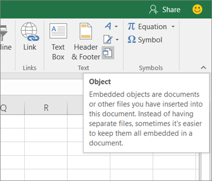
Insert a link to a file

You might want to just add a link to the object rather than fully embedding it. You can do that if your workbook and the object you want to add are both stored on a SharePoint site, a shared network drive, or a similar location, and if the location of the files will remain the same. This is handy if the linked object undergoes changes because the link always opens the most up-to-date document.

Note: If you move the linked file to another location, the link won’t work anymore.

Click inside the cell of the spreadsheet where you want to insert the object.
On the Insert tab, in the Text group, click Object .
Click the Create from File tab.
Click Browse, and then select the file you want to link.
Select the Link to file check box, and click OK.

Create a new object from inside Excel

You can create an entirely new object based on another program without leaving your workbook. For example, if you want to add a more detailed explanation to your chart or table, you can create an embedded document, such as a Word or PowerPoint file, in Excel. You can either set your object to be displayed right in a worksheet or add an icon that opens the file.

Click inside the cell of the spreadsheet where you want to insert the object.
On the Insert tab, in the Text group, click Object .
On the Create New tab, select the type of object you want to insert from the list presented. If you want to insert an icon into the spreadsheet instead of the object itself, select the Display as icon check box.
Click OK. Depending on the type of file you are inserting, either a new program window opens or an editing window appears within Excel.
Create the new object you want to insert.

When you’re done, if Excel opened a new program window in which you created the object, you can work directly within it.

When you’re done with your work in the window, you can do other tasks without saving the embedded object. When you close the workbook your new objects will be saved automatically.

Note: After you add the object, you can drag and drop it anywhere on your Excel worksheet. You can also resize the object by using the resizing handles. To find the handles, click the object one time.

Embed an object in a worksheet

Click inside the cell of the spreadsheet where you want to insert the object.
On the Insert tab, in the Text group, click Object.
Click the Create from File tab.
Click Browse, and select the file you want to insert.
If you want to insert an icon into the spreadsheet instead of show the contents of the file, select the Display as icon check box. If you don’t select any check boxes, Excel shows the first page of the file. In both cases, the complete file opens with a double click. Click OK.

Note: After you add the icon or file, you can drag and drop it anywhere on the worksheet. You can also resize the icon or file by using the resizing handles. To find the handles, click the file or icon one time.

Insert a link to a file

Note: If you move the linked file to another location, the link won’t work anymore.

Click inside the cell of the spreadsheet where you want to insert the object.
On the Insert tab, in the Text group, click Object.
Click the Create from File tab.
Click Browse, and then select the file you want to link.
Select the Link to file check box, and click OK.

Create a new object from inside Excel

Click inside the cell of the spreadsheet where you want to insert the object.
On the Insert tab, in the Text group, click Object.
On the Create New tab, select the type of object you want to insert from the list presented. If you want to insert an icon into the spreadsheet instead of the object itself, select the Display as icon check box.
Click OK. Depending on the type of file you are inserting, either a new program window opens or an editing window appears within Excel.
Create the new object you want to insert.

When you’re done, if Excel opened a new program window in which you created the object, you can work directly within it.

When you’re done with your work in the window, you can do other tasks without saving the embedded object. When you close the workbook your new objects will be saved automatically.

Note: After you add the object, you can drag and drop it anywhere on your Excel worksheet. You can also resize the object by using the resizing handles. To find the handles, click the object one time.

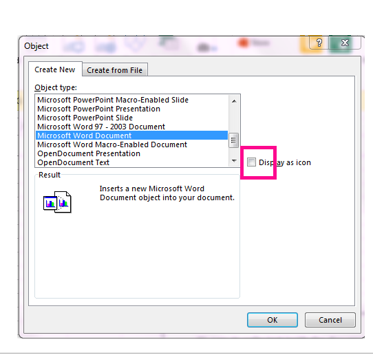
Link or embed content from another program by using OLE

You can link or embed all or part of the content from another program.

Create a link to content from another program

Click in the worksheet where you want to place the linked object.
On the Insert tab, in the Text group, click Object.
Click the Create from File tab.
In the File name box, type the name of the file, or click Browse to select from a list.
Select the Link to file check box.
Do one of the following:
- To display the content, clear the Display as icon check box.
- To display an icon, select the Display as icon check box. Optionally, to change the default icon image or label, click Change Icon, and then click the icon that you want from the Icon list, or type a label in the Caption box.
Note: You cannot use the Object command to insert graphics and certain types of files. To insert a graphic or file, on the Insert tab, in the Illustrations group, click Picture.

Embed content from another program

Click in the worksheet where you want to place the embedded object.
On the Insert tab, in the Text group, click Object.
If the document does not already exist, click the Create New tab. In the Object type box, click the type of object that you want to create.

If the document already exists, click the Create from File tab. In the File name box, type the name of the file, or click Browse to select from a list.
Clear the Link to file check box.
Do one of the following:
- To display the content, clear the Display as icon check box.
- To display an icon, select the Display as icon check box. To change the default icon image or label, click Change Icon, and then click the icon that you want from the Icon list, or type a label in the Caption box.

Link or embed partial content from another program

From a program other than Excel, select the information that you want to copy as a linked or embedded object.
On the Home tab, in the Clipboard group, click Copy.
Switch to the worksheet that you want to place the information in, and then click where you want the information to appear.
On the Home tab, in the Clipboard group, click the arrow below Paste, and then click Paste Special.
Do one of the following:
- To paste the information as a linked object, click Paste link.
- To paste the information as an embedded object, click Paste. In the As box, click the entry with the word «object» in its name. For example, if you copied the information from a Word document, click Microsoft Word Document Object.

Change the way that an OLE object is displayed

Right-click the icon or object, point to object typeObject (for example, Document Object), and then click Convert.
Do one of the following:
- To display the content, clear the Display as icon check box.
- To display an icon, select the Display as icon check box. Optionally, you can change the default icon image or label. To do that, click Change Icon, and then click the icon that you want from the Icon list, or type a label in the Caption box.

Control updates to linked objects

You can set links to other programs to be updated in the following ways: automatically, when you open the destination file; manually, when you want to see the previous data before updating with the new data from the source file; or when you specifically request the update, regardless of whether automatic or manual updating is turned on.

Set a link to another program to be updated manually

On the Data tab, in the Connections group, click Edit Links.

Note: The Edit Links command is unavailable if your file does not contain links to other files.
In the Source list, click the linked object that you want to update. An A in the Update column means that the link is automatic, and an M in the Update column means that the link is set to Manual update.

Tip: To select multiple linked objects, hold down CTRL and click each linked object. To select all linked objects, press CTRL+A.
To update a linked object only when you click Update Values, click Manual.

Set a link to another program to be updated automatically

On the Data tab, in the Connections group, click Edit Links.

Note: The Edit Links command is unavailable if your file does not contain links to other files.
In the Source list, click the linked object that you want to update. An A in the Update column means that the link will update automatically, and an M in the Update column means that the link must be updated manually.

Tip: To select multiple linked objects, hold down CTRL and click each linked object. To select all linked objects, press CTRL+A.
Click OK.

Issue: I can’t update the automatic links on my worksheet

The Automatic option can be overridden by the Update links to other documents Excel option.

To ensure that automatic links to OLE objects can be automatically updated:

Click the Microsoft Office Button , click Excel Options, and then click the Advanced category.
Under When calculating this workbook, make sure that the Update links to other documents check box is selected.

Update a link to another program now

On the Data tab, in the Connections group, click Edit Links.

Note: The Edit Links command is unavailable if your file does not contain linked information.
In the Source list, click the linked object that you want to update.

Tip: To select multiple linked objects, hold down CTRL and click each linked object. To select all linked objects, press CTRL+A.
Click Update Values.

Edit content from an OLE program

While you are in Excel, you can change the content linked or embedded from another program.

Edit a linked object in the source program

On the Data tab, in the Connections group, click Edit Links.

Note: The Edit Links command is unavailable if your file does not contain linked information.
In the Source file list, click the source for the linked object, and then click Open Source.
Make the changes that you want to the linked object.
Exit the source program to return to the destination file.

Edit an embedded object in the source program

Double-click the embedded object to open it.
Make the changes that you want to the object.
If you are editing the object in place within the open program, click anywhere outside of the object to return to the destination file.

If you edit the embedded object in the source program in a separate window, exit the source program to return to the destination file.

Note: Double-clicking certain embedded objects, such as video and sound clips, plays the object instead of opening a program. To edit one of these embedded objects, right-click the icon or object, point to object typeObject (for example, Media Clip Object), and then click Edit.

Edit an embedded object in a program other than the source program

Select the embedded object that you want to edit.
Right-click the icon or object, point to object typeObject (for example, Document Object), and then click Convert.
Do one of the following:
- To convert the embedded object to the type that you specify in the list, click Convert to.
- To open the embedded object as the type that you specify in the list without changing the embedded object type, click Activate.

Select an OLE object by using the keyboard

Press CTRL+G to display the Go To dialog box.
Click Special, select Objects, and then click OK.
Press TAB until the object that you want is selected.
Press SHIFT+F10.
Point to Object or Chart Object, and then click Edit.

Issue: When I double-click a linked or embedded object, a «cannot edit» message appears

This message appears when the source file or source program can’t be opened.

Make sure that the source program is available If the source program is not installed on your computer, convert the object to the file format of a program that you do have installed.

Ensure that memory is adequate Make sure that you have enough memory to run the source program. Close other programs to free up memory, if necessary.

Close all dialog boxes If the source program is running, make sure that it doesn’t have any open dialog boxes. Switch to the source program, and close any open dialog boxes.

Close the source file If the source file is a linked object, make sure that another user doesn’t have it open.

Ensure that the source file name has not changed If the source file that you want to edit is a linked object, make sure that it has the same name as it did when you created the link and that it has not been moved. Select the linked object, and then click the Edit Links command in the Connections group on the Data tab to see the name of the source file. If the source file has been renamed or moved, use the Change Source button in the Edit Links dialog box to locate the source file and reconnect the link.

Need more help?

You can always ask an expert in the Excel Tech Community or get support in the Answers community.

Источник

Calculating Combinations
The COMBIN function is used to determine the number of combinations that can be made from a group of elements. This tip explains the function and how you can use it.

Calculating the Day of the Year
Need to know what day of the year a certain date is? You can figure it out easily using the formulas in this tip.

Checking for Text
Need to figure out if a particular cell contains text? You can use the ISTEXT function to easily return this bit of trivia.

Cleaning Text
You can use the CLEAN worksheet function to remove any non-printable characters from a cell. This can come in handy when you want to pare down what is stored in a worksheet.

Colors in an IF Function
You can use the IF worksheet function to test for a number of different conditions or values. You can’t use it to check for cell colors, however. Here are some ideas on how you can take cell colors into account in the IF function.

Converting Codes to Characters
Character codes are the numeric values used, by a computer, to signify various alphanumeric characters. You can use the CHAR worksheet function to discover the character code of any character.

Converting Radians to Degrees
When applying trigonometry to the values in a worksheet, you may need to convert radians to degrees. This is done by using the DEGREES worksheet function, described in this tip.

Converting to Hexadecimal
Excel allows you to easily convert values from decimal to other numbering systems, such as hexadecimal. This tip explains how to use the DEC2HEX worksheet function.

Converting to Octal
If you need to do some work in the base-8 numbering system (octal), you’ll love two worksheet functions provided by Excel for this purpose. These functions allow you to convert values to octal and convert them back again.

Converting to Other Number Systems
Most calculations are done using the decimal numbering system. If you need to convert your decimal values to a differing numbering system, then you’ll appreciate the functions discussed in this tip.

Counting Displayed Cells
When you filter data, Excel displays only a portion of what is really in a worksheet. If you want to count the number of cells that are displayed after filtering, then you’ll want to explore the techniques in this tip.

Counting the Number of Blank Cells
If you need to count the number of blank cells in a range, the function to use is COUNTBLANK. This tip discusses the function, along with a «gotcha» that you should be aware of.

Counting with Formulas
When you need to count a number of cells based upon a single criteria, the standard function to use is COUNTIF. This tip explains, through an example, how you can use the function to do the desired counting.

Determining a Value of a Cell
Cells can store all sorts of information that can be formatted and displayed in a myriad of ways. If you want to quickly get to the value stored within the cell, you can use the N worksheet function.

Determining Columns in a Range
If you need to know the number of columns in a particular range, you can use the COLUMNS worksheet function. This tip demonstrates how simple it is to use the function.

Determining the Least Common Multiple
Need to figure out the least common multiple of a range of values? It is a snap when you use the LCM function, described in this tip.

Disabling #SPILL! Errors
In the newest version of Excel, a change in how formulas are calculated can cause havoc for some «older» formulas. Here is why that happens and what you can do about it.

Displaying Letter Grades
Grading in schools is often done using numeric values. However, you may want to change those numeric values into letter grades based upon a determined scale. This can be done most easily using Excel’s lookup functions.

EOMONTH Function is Flakey
Some users have reported problems using the EOMONTH function in later versions of Excel, beginning with Excel 2007. The problem seems to be related to Excel’s compatibility mode and the fact that the function was moved from the Analysis ToolPak to Excel itself.

Establishing a FLOOR and CEILING
Excel includes a surprising number of functions you can use to round your data. Two such functions are FLOOR and CEILING, described in this tip.

Exact Matches with DSUM
The DSUM function is very handy when you need to calculate a sum based on data that matches criteria you specify. If you don’t specify the criteria just right, however, you may not get the results you expect.

Finding the Date Associated with a Negative Value
When working with data taken from the real world, you often have to determine which certain conditions were met, such as when a particular reading dropped below a certain value. This tip examines how you can easily tell the date on which a reading drops below zero.

Finding the Lowest Numbers
Need to find the lowest numbers in a range of values? It’s easy to do using the SMALL worksheet function, or you can use a macro for more demanding needs.

Finding the Nth Root of a Number
Finding a square root is easy because Excel provides a worksheet function for that purpose. Finding a different root may not be as easy, unless you adapt the formula presented in this tip.

Finding Unique Rows Based on Two Columns
Using the UNIQUE function you can derive unique values from a range of cells. By expanding the range of cells accessed by the function you can control what is returned.

Getting Help when Entering Functions
Need a quick memory jog when entering a worksheet function? Here’s a shortcut that will be invaluable.

Getting the Name of the Parent Workbook
If you need to insert into a cell the name of the workbook in which a worksheet is contained, you can use the CELL function. This tip explains the proper way to get the info you need.

Indirect References to a DSUM Parameter
Indirect references can be very helpful in formulas, but getting your head around how they work can sometimes be confusing. Here’s an example of using an indirect reference within another formula.

Leaving a Cell Value Unchanged If a Condition Is False
Ever want the IF function to only return a value if the condition it is testing is true, and not if the condition is false? This tip explains how this function works and what you can do to only return what you are looking for.

Making PROPER Skip Certain Words
The PROPER worksheet function is used to change the case of text so that only the first letter of each word is uppercase. However, some words should not have the initial letter uppercased. There are a couple of ways you can modify the work done by PROPER, as described in this tip.

Making VLOOKUP Case Sensitive
The VLOOKUP function, like other lookup functions in Excel, is not case sensitive. In other words, it doesn’t matter whether the characters being evaluated are upper- or lower-case. If you need the function to pay attention to character case, then you will need to devise a workaround. The techniques in this tip are a great place to start.

Making VLOOKUP Trigger a Macro
VLOOKUP is an oft-used worksheet function to lookup values in a data table. If the function cannot return a value, it normally returns an error. This knowledge can help you figure out how to run a macro when VLOOKUP fails.

Making Your Formulas Check for Errors
Want to use a formula to check if there is an error in your formula? (Sounds confusing, but it’s not that bad.) You’ll love the IFERROR function, described in this tip.

Median of Selected Numbers
Need to find a median value in a series of values? It’s easy with the MEDIAN function. What isn’t as easy is to derive the median from only a subset of the values based upon some criterion. Here’s an easy way to approach the task.

Modifying Proper Capitalization
The PROPER worksheet function is used to change the case of text so that the first letter of each word is capitalized. If there are some words you don’t want to have an initial cap, then you’ll want to use the ideas presented in this tip.

Nesting IF Worksheet Functions
The IF worksheet function is very handy to make conditional evaluations. You are not limited to a single IF comparison, however. Excel allows you to easily nest IF statements within each other.

Outstanding Macro Function Reference
Looking for a great reference that you can use to help figure out the various worksheet functions available in Excel? Here’s a free resource you need to check.

Phantom Counts
Two common worksheet functions used to count things are COUNT and COUNTA. Not understanding how these functions treat cell contents can result in incorrect counts.

Random Numbers in a Range
Excel provides several different functions that you can use to generate random numbers. One of the most useful is the RANDBETWEEN function, which allows you to generate a random number between a lower and upper boundary that you specify.

Returning an ANSI Value
Need to know the character value of the first character in a string? It’s easy to do, without using a macro, by using the CODE function, described in this tip.

Returning Blanks or Asterisks from a Lookup
Want to return more than a value when doing a lookup? Here are a couple of ways to do it by adding an IF clause to your formula.

Returning Blanks with VLOOKUP
Normally the VLOOKUP function returns a value, and if it can’t return a value it returns a zero. Here’s how you can use the function within a formula to be more discriminating in what is returned.

Returning Item Codes Instead of Item Names
The data validation capabilities of Excel are really handy when you want to limit what is put into a cell. However, you can’t use data validation to return a value different than what the user selects. There are ways around this, though.

Returning the Left-most Characters
When working with text in a formula, you may need to extract the left-most characters from a string of text or from a cell. You can do this using the LEFT worksheet function, described in this tip.

Returning the MODE of a Range
The MODE function is used to determine the most frequently recurring value in a range. This tip explains how to use the function in your worksheet.

Returning Values to the Left of a VLOOKUP
VLOOKUP is a great function to use in accessing data based on a lookup value. Problem is, you can’t easily return information to the left of the cell in which you are looking up values. This tip focuses on three approaches to getting around this limitation.

Selecting Random Names
Got a ton of names from which you need to select a few random names? There are several ways you can extract what you need; several different ideas are explained in this tip.

Specifying a Date Range in a SUMIFS Formula
The SUMIFS function allows you to specify criteria by which values can be included in a sum. Putting together the criteria for the function can be confusing, though, when working with dates. This tip provides a step-by-step look at how you can specify the criteria properly.

Specifying a Language for the TEXT Function
You may want to use Excel to display dates using a different language than your normal one. There are a couple of ways you can go about this, as described in this tip.

Specifying Proper Case
If you need to change the case of letters in a cell, one of the functions you can use is the PROPER function. This tip describes how to use the function to alter the appearance of your text.

Strange ATAN Results
You may use Excel’s trigonometric functions to do some quick calculations, and suddenly notice that the results in your worksheet are different than the results you get using a calculator. The reason could be as simple as understanding what Excel expects in its functions.

The EDATE Function
Want to figure a date a certain number of months in the future or past? The EDATE function may be just what you need for your calculation.

Understanding the VLOOKUP Function
Functions are at the heart of Excel’s power in working with data. One of the most misunderstood functions provided by Excel is VLOOKUP. Here’s a brief overview of how to use the function.

Using a Cell Value as a Worksheet Name in a Formula
Excel allows you to easily develop formulas that pull values from worksheets and workbooks other than the one in which you are working. A great way to put together such a formula is through the use of the INDIRECT function, described in this tip.

Using a Week Number as One Criterion in a Formula
The SUMIFS function can be quite powerful in conditionally summing information based on criteria you specify. This tip looks at one example of using the function based on two criteria, one of which is the week number of the dates associated with some values.

Using COUNTIF with Colors
Excel allows you to easily format cells with different fonts, borders, and colors. If you want to count the number of cells that use a particular background color, there are a couple of approaches you can use. This tip shows you how.

Using GEOMEAN with a Large List
When performing a statistical analysis on a large dataset, you may want to use GEOMEAN to figure out the geometric mean of the data. Doing so, however, could possibly generate an error, as described in this tip.

Using the ABS Function
Need to find the absolute value of a number? That’s where the ABS function comes into play.

Using the COLUMN Function
Need to know the column number for use in a formula? The worksheet function you want is the COLUMN function, described in this tip.

Using the CONCATENATE Worksheet Function
The process of combining string (text) values to make a new string is called concatenation. Excel provides the CONCATENATE function to accomplish the task, but there is an even easier way to join strings together.

Using the EOMONTH Function
If you need to determine the date of the last day in a month, it’s hard to beat the flexibility of the EOMONTH function. This tip explains how to use this function in your formulas.

Using the FORECAST Function
Excel provides a handy worksheet function that allows you to forecast values based upon a set of known values. This function, appropriately enough, is known as the FORECAST function and is described in this tip.

Using the IF Worksheet Function
Programmers know that a staple of any language is the ability to create conditional statements. Excel understands this, as well, so it provides the IF worksheet function that allows you to evaluate an expression and thereby conditionally choose a result.

Using the INT Worksheet Function
The INT function allows you to convert a value to an integer. The effect the function has depends on the characteristics of the number it is converting.

Using the IRR Function
When working with finances, you often need to know the rate of return on a given investment. The most common type of calculation used is the internal rate of return, which in Excel is calculated using the IRR worksheet function.

Using the REPT Function
Excel includes a handy function that allows you to repeat characters or strings of characters. How you use the REPT function is presented in this tip.

Using the TRUNC Worksheet Function
Want to chop off everything after a certain point in a number? The TRUNC function can help with this need.

Using the UNIQUE Function
The UNIQUE function can be used to evaluate a range and return the unique values in that range. Understanding how the function works, as described in this tip, can allow you to do even more with UNIQUE.

Using the WEEKNUM Function
Need to know which week of the year a particular date falls within? Excel provides the WEEKNUM function so you can easily calculate this statistic.

Using the XIRR Function
One of the financial worksheet functions provided in Excel is the XIRR function. This is used to figure out an internal rate of return when the payments associated with an investment are not evenly spaced. Here’s how to use the function.

Ways to Concatenate Values
Users of the most recent versions of Excel have four different ways available to combine values into strings. Even those using older versions have two ways they can use. So how do these concatenation techniques compare to each other? This tip provides the info you need.

Источник

Apart from cells and ranges, working with worksheets is another area you should know about to use VBA efficiently in Excel.

Just like any object in VBA, worksheets have different properties and methods associated with it that you can use while automating your work with VBA in Excel.

In this tutorial, I will cover ‘Worksheets’ in detail and also show you some practical examples.

So let’s get started.

All the codes I mention in this tutorial need to be placed in the VB Editor. Go to the ‘Where to Put the VBA Code‘ section to know how it works.

If you’re interested in learning VBA the easy way, check out my Online Excel VBA Training.

Difference between Worksheets and Sheets in VBA
Referencing a Worksheet in VBA
- Using the Worksheet Name
- Using the Index Number
- Using the Worksheet Code Name
- Referring to a Worksheet in a Different Workbook
Adding a Worksheet
Deleting a Worksheet
Renaming the Worksheets
Assigning Worksheet Object to a Variable
Hide Worksheets Using VBA (Hidden + Very Hidden)
Hide Sheets Based on the Text in it
Sorting the Worksheets in an Alphabetical Order
Protect/Unprotect All the Sheets at One Go
Creating a Table of Contents of All Worksheets (with Hyperlinks)
Where to Put the VBA Code

Difference between Worksheets and Sheets in VBA

In VBA, you have two collections that can be a bit confusing at times.

In a workbook, you can have worksheets and as well as chart sheets. The example below has three worksheets and one chart sheet.

In Excel VBA:

The ‘Worksheets’ collection would refer to the collection of all the worksheet objects in a workbook. In the above example, the Worksheets collection would consist of three worksheets.
The ‘Sheets’ collection would refer to all the worksheets as well as chart sheets in the workbook. In the above example, it would have four elements – 3 Worksheets + 1 Chart sheet.

If you have a workbook that only has worksheets and no chart sheets, then ‘Worksheets’ and ‘Sheets’ collection is the same.

But when you have one or more chart sheets, the ‘Sheets’ collection would be bigger than the ‘Worksheets’ collection

Sheets = Worksheets + Chart Sheets

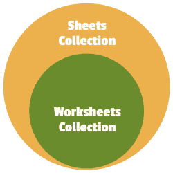
Now with this distinction, I recommend being as specific as possible when writing a VBA code.

So if you have to refer to worksheets only, use the ‘Worksheets’ collection, and if you have to refer to all sheets (including chart sheets), the use the ‘Sheets’ collection.

In this tutorial, I will be using the ‘Worksheets’ collection only.

Referencing a Worksheet in VBA

There are many different ways you can use to refer to a worksheet in VBA.

Understanding how to refer to worksheets would help you write better code, especially when you’re using loops in your VBA code.

Using the Worksheet Name

The easiest way to refer to a worksheet is to use its name.

For example, suppose you have a workbook with three worksheets – Sheet 1, Sheet 2, Sheet 3.

And you want to activate Sheet 2.

You can do that using the following code:

Sub ActivateSheet()
Worksheets("Sheet2").Activate
End Sub

The above code asks VBA to refer to Sheet2 in the Worksheets collection and activate it.

Since we are using the exact sheet name, you can also use the Sheets collection here. So the below code would also do that same thing.

Sub ActivateSheet()
Sheets("Sheet2").Activate
End Sub

Using the Index Number

While using the sheet name is an easy way to refer to a worksheet, sometimes, you may not know the exact name of the worksheet.

For example, if you’re using a VBA code to add a new worksheet to the workbook, and you don’t know how many worksheets are already there, you would not know the name of the new worksheet.

In this case, you can use the index number of the worksheets.

Suppose you have the following sheets in a workbook:

The below code would activate Sheet2:

Sub ActivateSheet()
Worksheets(2).Activate
End Sub

Note that we have used index number 2 in Worksheets(2). This would refer to the second object in the collection of the worksheets.

Now, what happens when you use 3 as the index number?

It will select Sheet3.

If you’re wondering why it selected Sheet3, as it’s clearly the fourth object.

This happens because a chart sheet is not a part of the worksheets collection.

So when we use the index numbers in the Worksheets collection, it will only refer to the worksheets in the workbook (and ignore the chart sheets).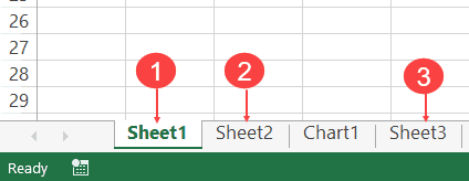

On the contrary, if you’re using Sheets, Sheets(1) would refer to Sheets1, Sheets(2) would refer to Sheet2, Sheets(3) would refer to Chart1 and Sheets(4) would refer to Sheet3.

This technique of using index number is useful when you want to loop through all the worksheets in a workbook. You can count the number of worksheets and then loop through these using this count (we will see how to do this later in this tutorial).

Note: The index number goes from left to right. So if you shift Sheet2 to the left of Sheet1, then Worksheets(1) would refer to Sheet2.

Using the Worksheet Code Name

One of the drawbacks of using the sheet name (as we saw in the section above) is that a user can change it.

And if the sheet name has been changed, your code wouldn’t work until you change the name of the worksheet in the VBA code as well.

To tackle this problem, you can use the code name of the worksheet (instead of the regular name that we have been using so far). A code name can be assigned in the VB Editor and doesn’t change when you change the name of the sheet from the worksheet area.

To give your worksheet a code name, follow the below steps:

Click the Developer tab.
Click the Visual Basic button. This will open the VB Editor.
Click the View option in the menu and click on Project Window. This will make the Properties pane visible. If the Properties pane is already visible, skip this step.
Click on the sheet name in the project explorer that you want to rename.
In the Properties pane, change the name in the field in front of (Name). Note that you can’t have spaces in the name.

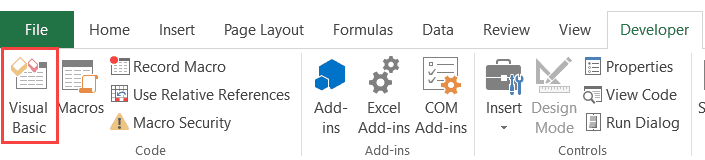
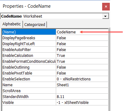
The above steps would change the name of your Worksheet in the VBA backend. In the Excel worksheet view, you can name the worksheet whatever you want, but in the backend, it will respond to both the names – the sheet name and the code name.

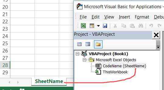
In the above image, the sheet name is ‘SheetName’ and the code name is ‘CodeName’. Even if you change the sheet name on the worksheet, the code name still remains the same.

Now, you can use either the Worksheets collection to refer to the worksheet or use the codename.

For example, both the line will activate the worksheet.

Worksheets("Sheetname").Activate
CodeName.Activate

The difference in these two is that if you change the name of the worksheet, the first one wouldn’t work. But the second line would continue to work even with the changed name. The second line (using the CodeName) is also shorter and easier to use.

Referring to a Worksheet in a Different Workbook

If you want to refer to a worksheet in a different workbook, that workbook needs to be open while the code runs, and you need to specify the name of the workbook and the worksheet that you want to refer to.

For example, if you have a workbook with the name Examples and you want to activate Sheet1 in the Example workbook, you need to use the below code:

Sub SheetActivate()
Workbooks("Examples.xlsx").Worksheets("Sheet1").Activate
End Sub

Note that if the workbook has been saved, you need to use the file name along with the extension. If you’re not sure what name to use, take help from Project Explorer.

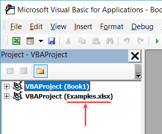
In case the workbook has not been saved, you don’t need to use the file extension.

Adding a Worksheet

The below code would add a worksheet (as the first worksheet – i.e., as the leftmost sheet in the sheet tab).

Sub AddSheet()
Worksheets.Add
End Sub

It takes the default name Sheet2 (or any other number based on how many sheets are already there).

If you want a worksheet to be added before a specific worksheet (say Sheet2), then you can use the below code.

Sub AddSheet()
Worksheets.Add Before:=Worksheets("Sheet2")
End Sub

The above code tells VBA to add a sheet and then uses the ‘Before’ statement to specify the worksheet before which the new worksheet should to be inserted.

Similarly, you can also add a sheet after a worksheet (say Sheet2), using the below code:

Sub AddSheet()
Worksheets.Add After:=Worksheets("Sheet2")
End Sub

If you want the new sheet to be added to the end of the sheets, you need to first know how many sheets are there. The following code first counts the number of sheets, and the adds the new sheet after the last sheet (to which we refer using the index number).

Sub AddSheet()
Dim SheetCount As Integer
SheetCount = Worksheets.Count
Worksheets.Add After:=Worksheets(SheetCount)
End Sub

Deleting a Worksheet

The below code would delete the active sheet from the workbook.

Sub DeleteSheet()
ActiveSheet.Delete
End Sub

The above code would show a warning prompt before deleting the worksheet.

If you don’t want to see the warning prompt, use the below code:

Sub DeleteSheet()
Application.DisplayAlerts = False
ActiveSheet.Delete
Application.DisplayAlerts = True
End Sub

When Application.DisplayAlerts is set to False, it will not show you the warning prompt. If you use it, remember to set it back to True at the end of the code.

Remember that you can’t undo this delete, so use the above code when you’re absolutely sure.

If you want to delete a specific sheet, you can do that using the following code:

Sub DeleteSheet()
Worksheets("Sheet2").Delete
End Sub

You can also use the code name of the sheet to delete it.

Sub DeleteSheet()
Sheet5.Delete
End Sub

Renaming the Worksheets

You can modify the name property of the Worksheet to change its name.

The following code will change the name of Sheet1 to ‘Summary’.

Sub RenameSheet()
Worksheets("Sheet1").Name = "Summary"
End Sub

You can combine this with the adding sheet method to have a set of sheets with specific names.

For example, if you want to insert four sheets with the name 2018 Q1, 2018 Q2, 2018 Q3, and 2018 Q4, you can use the below code.

Sub RenameSheet()
Dim Countsheets As Integer
Countsheets = Worksheets.Count
For i = 1 To 4
Worksheets.Add after:=Worksheets(Countsheets + i - 1)
Worksheets(Countsheets + i).Name = "2018 Q" & i
Next i
End Sub

In the above code, we first count the number of sheets and then use a For Next loop to insert new sheets at the end. As the sheet is added, the code also renames it.

Assigning Worksheet Object to a Variable

When working with worksheets, you can assign a worksheet to an object variable, and then use the variable instead of the worksheet references.

For example, if you want to add a year prefix to all the worksheets, instead of counting the sheets and the running the loop that many numbers of times, you can use the object variable.

Here is the code that will add 2018 as a prefix to all the worksheet’s names.

Sub RenameSheet()
Dim Ws As Worksheet
For Each Ws In Worksheets
Ws.Name = "2018 - " & Ws.Name
Next Ws
End Sub

The above code declares a variable Ws as the worksheet type (using the line ‘Dim Ws As Worksheet’).

Now, we don’t need to count the number of sheets to loop through these. Instead, we can use ‘For each Ws in Worksheets’ loop. This will allow us to go through all the sheets in the worksheets collection. It doesn’t matter whether there are 2 sheets or 20 sheets.

While the above code allows us to loop through all the sheets, you can also assign a specific sheet to a variable.

In the below code, we assign the variable Ws to Sheet2 and use it to access all of Sheet2’s properties.

Sub RenameSheet()
Dim Ws As Worksheet
Set Ws = Worksheets("Sheet2")
Ws.Name = "Summary"
Ws.Protect
End Sub

Once you set a worksheet reference to an object variable (using the SET statement), that object can be used instead of the worksheet reference. This can be helpful when you have a long complicated code and you want to change the reference. Instead of making the change everywhere, you can simply make the change in the SET statement.

Note that the code declares the Ws object as the Worksheet type variable (using the line Dim Ws as Worksheet).

Hide Worksheets Using VBA (Hidden + Very Hidden)

Hiding and Unhiding worksheets in Excel is a straightforward task.

You can hide a worksheet and the user would not see it when he/she opens the workbook. However, they can easily unhide the worksheet by right-clicking on any sheet tab.

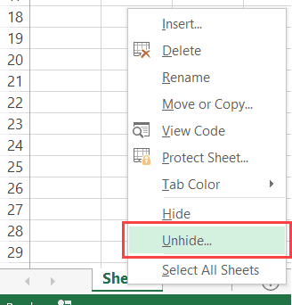
But what if you don’t want them to be able to unhide the worksheet(s).

You can do this using VBA.

The code below would hide all the worksheets in the workbook (except the active sheet), such that you can not unhide it by right-clicking on the sheet name.

Sub HideAllExcetActiveSheet()
Dim Ws As Worksheet
For Each Ws In ThisWorkbook.Worksheets
If Ws.Name <> ActiveSheet.Name Then Ws.Visible = xlSheetVeryHidden
Next Ws
End Sub

In the above code, the Ws.Visible property is changed to xlSheetVeryHidden.

When the Visible property is set to xlSheetVisible, the sheet is visible in the worksheet area (as worksheet tabs).
When the Visible property is set to xlSheetHidden, the sheet is hidden but the user can unhide it by right-clicking on any sheet tab.
When the Visible property is set to xlSheetVeryHidden, the sheet is hidden and cannot be unhidden from worksheet area. You need to use a VBA code or the properties window to unhide it.

If you want to simply hide sheets, that can be unhidden easily, use the below code:

Sub HideAllExceptActiveSheet()
Dim Ws As Worksheet
For Each Ws In ThisWorkbook.Worksheets
If Ws.Name <> ActiveSheet.Name Then Ws.Visible = xlSheetHidden
Next Ws
End Sub

The below code would unhide all the worksheets (both hidden and very hidden).

Sub UnhideAllWoksheets()
Dim Ws As Worksheet
For Each Ws In ThisWorkbook.Worksheets
Ws.Visible = xlSheetVisible
Next Ws
End Sub

Related Article: Unhide All Sheets In Excel (at one go)

Hide Sheets Based on the Text in it

Suppose you have multiple sheets with the name of different departments or years and you want to hide all the sheets except the ones that have the year 2018 in it.

You can do this using a VBA INSTR function.

The below code would hide all the sheets except the ones with the text 2018 in it.

Sub HideWithMatchingText()
Dim Ws As Worksheet
For Each Ws In Worksheets
If InStr(1, Ws.Name, "2018", vbBinaryCompare) = 0 Then
Ws.Visible = xlSheetHidden
End If
Next Ws
End Sub

In the above code, the INSTR function returns the position of the character where it finds the matching string. If it doesn’t find the matching string, it returns 0.

The above code checks whether the name has the text 2018 in it. If it does, nothing happens, else the worksheet is hidden.

You can take this a step further by having the text in a cell and using that cell in the code. This will allow you to have a value in the cell and then when you run the macro, all the sheets, except the one with the matching text in it, would remain visible (along with the sheets where you’re entering the value in the cell).

Sorting the Worksheets in an Alphabetical Order

Using VBA, you can quickly sort the worksheets based on their names.

For example, if you have a workbook that has sheets for different department or years, then you can use the below code to quickly sort these sheets in an ascending order.

Sub SortSheetsTabName()
Application.ScreenUpdating = False
Dim ShCount As Integer, i As Integer, j As Integer
ShCount = Sheets.Count
For i = 1 To ShCount - 1
For j = i + 1 To ShCount
If Sheets(j).Name < Sheets(i).Name Then
Sheets(j).Move before:=Sheets(i)
End If
Next j
Next i
Application.ScreenUpdating = True
End Sub

Note that this code works well with text names and in most of the cases with years and numbers too. But it can give you the wrong results in case you have the sheet names as 1,2,11. It will sort and give you the sequence 1, 11, 2. This is because it does the comparison as text and considers 2 bigger than 11.

Protect/Unprotect All the Sheets at One Go

If you have a lot of worksheets in a workbook and you want to protect all the sheets, you can use the VBA code below.

It allows you to specify the password within the code. You will need this password to unprotect the worksheet.

Sub ProtectAllSheets()
Dim ws As Worksheet
Dim password As String
password = "Test123" 'replace Test123 with the password you want
For Each ws In Worksheets
ws.Protect password:=password
Next ws
End Sub

The following code would unprotect all the sheets in one go.

Sub ProtectAllSheets()
Dim ws As Worksheet
Dim password As String
password = "Test123" 'replace Test123 with the password you used while protecting
For Each ws In Worksheets
ws.Unprotect password:=password
Next ws
End Sub

Creating a Table of Contents of All Worksheets (with Hyperlinks)

If you have a set of worksheets in the workbook and you want to quickly insert a summary sheet which has the links to all the sheets, you can use the below code.

Sub AddIndexSheet()
Worksheets.Add
ActiveSheet.Name = "Index"
For i = 2 To Worksheets.Count
ActiveSheet.Hyperlinks.Add Anchor:=Cells(i - 1, 1), _
Address:="", SubAddress:=Worksheets(i).Name & "!A1", _
TextToDisplay:=Worksheets(i).Name
Next i
End Sub

The above code inserts a new worksheet and names it Index.

It then loops through all the worksheets and creates a hyperlink for all the worksheets in the Index sheet.

Where to Put the VBA Code

Wondering where the VBA code goes in your Excel workbook?

Excel has a VBA backend called the VBA editor. You need to copy and paste the code into the VB Editor module code window.

Here are the steps to do this:

Go to the Developer tab.
Click on the Visual Basic option. This will open the VB editor in the backend.
In the Project Explorer pane in the VB Editor, right-click on any object for the workbook in which you want to insert the code. If you don’t see the Project Explorer go to the View tab and click on Project Explorer.
Go to Insert and click on Module. This will insert a module object for your workbook.
Copy and paste the code in the module window.

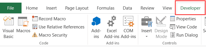
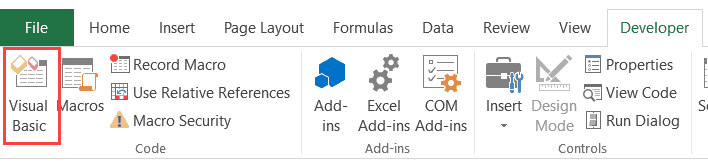
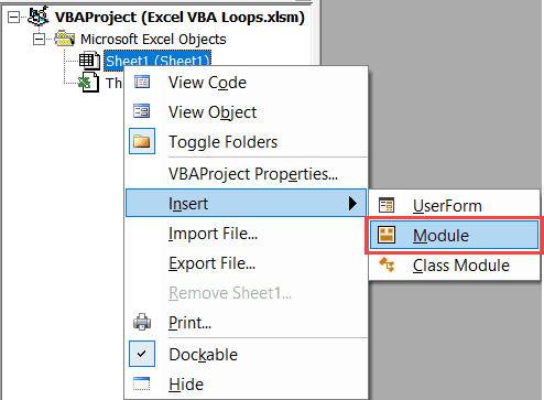
You May Also Like the Following Excel VBA Tutorials:

Working with Workbooks using VBA.
Using IF Then Else Statements in VBA.
For Next Loop in VBA.
Creating a User-Defined Function in Excel.
How to Record a Macro in Excel.
How to Run a Macro in Excel.
Excel VBA Events – An Easy (and Complete) Guide.
How to Create an Add-in in Excel.
How to Save and Reuse Macro using Excel Personal Macro Workbook.
Using Active Cell in VBA in Excel (Examples)
How to Open Excel Files Using VBA (Examples)

Источник