
Excel for Microsoft 365 Excel 2021 Excel 2019 Excel 2016 More…Less
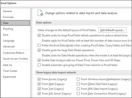
Beginning with Excel 2016 for Office 365 subscribers, The Data import and analysis options have been moved to their own Data section in the Excel Options dialog box. You can reach these options by selecting File > Options > Data. In earlier versions of Excel, the Data tab can be found by selecting File > Options > Advanced.
Data Options
-
Make changes to the default layout for Pivot Tables.
You can choose from multiple default layout options for new PivotTables. For instance, you can choose to always create a new PivotTable in Tabular Form versus Compact, or turn off Autofit column widths on update.
-
Disable undo for large PivotTable refresh operations to reduce refresh time.
If you choose to disable undo, you can select the number of rows as a threshold for when to disable it. The default is 300,000 rows.
-
Prefer the Excel Data Model when creating PivotTables, Query Tables and Data Connections.
The Data Model integrates data from multiple tables, effectively building a relational data source inside an Excel workbook.
-
Disable undo for large Data Model operations.
If you choose to disable undo, you can select the number of megabytes in file size as a threshold for when to disable it. The default is 8 Mb.
-
Enable Data Analysis add-ins: Power Pivot, Power View and 3D Maps.
Enable Data Analysis add-ins here instead of through the Add-ins tab.
-
Disable automatic grouping of Date/Time columns in PivotTables.
By default, date and time columns get grouped with + signs next to them. This setting will disable that default.
Show legacy data import wizards
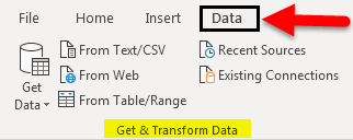
Power Query (formerly Get & Transform) available through the Data tab on the ribbon, is superior in terms of data connectors and transformational capabilities compared to the legacy data import wizards. However, there may still be times when you want to use one of these wizards to import your data. For example, when you want to save the data source login credentials as part of your workbook.
Security Saving credentials is not recommended and may lead to security and privacy issues or compromised data.
To enable the legacy data import wizards
-
Select File > Options > Data.
-
Select one or more wizards to enable access from the Excel ribbon.

-
Close the workbook and then reopen it to see the activate the wizards
-
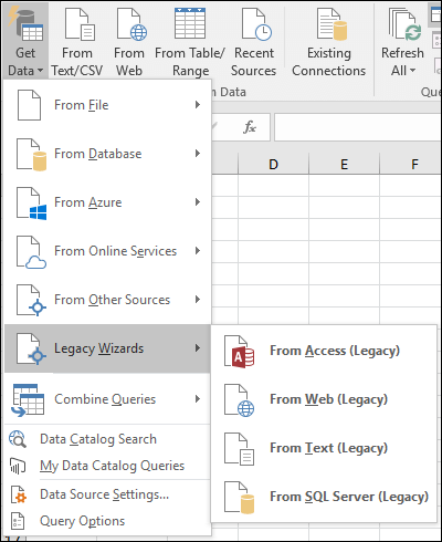
Select Data > Get Data > Legacy Wizards, and then select the wizard you want.
You can disable the wizards by repeating steps 1 through 3, but clearing the check boxes described in step 2.
See Also
Power Query in Excel
Set PivotTable default layout options
Create a Data Model in Excel
Need more help?
Want more options?
Explore subscription benefits, browse training courses, learn how to secure your device, and more.
Communities help you ask and answer questions, give feedback, and hear from experts with rich knowledge.
Содержание
- Data import and analysis options
- Data Options
- Show legacy data import wizards
- Text Import Wizard
- Step 1 of 3
- Step 2 of 3 (Delimited data)
- Step 2 of 3 (Fixed width data)
- Step 3 of 3
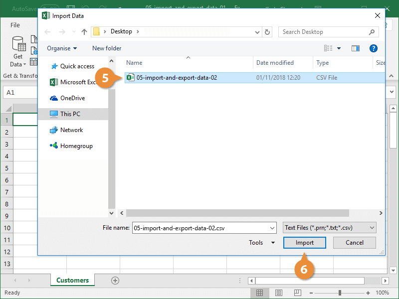
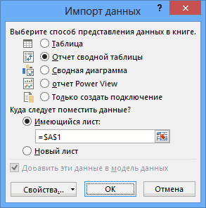
- Import Data
- Step 1 of 3
- Step 2 of 3 (Delimited data)
- Step 2 of 3 (Fixed width data)
- Step 3 of 3
- Import Data
- Need more help?
Data import and analysis options
Beginning with Excel 2016 for Office 365 subscribers, The Data import and analysis options have been moved to their own Data section in the Excel Options dialog box. You can reach these options by selecting File > Options > Data. In earlier versions of Excel, the Data tab can be found by selecting F ile > Options > Advanced.
Options > Advanced section to a new tab called Data under File > Options.» loading=»lazy»>
Note: This feature is only available if you have an Office 365 subscription. If you are an Microsoft 365 subscriber, make sure you have the latest version of Office.
Data Options
Make changes to the default layout for Pivot Tables.
You can choose from multiple default layout options for new PivotTables. For instance, you can choose to always create a new PivotTable in Tabular Form versus Compact, or turn off Autofit column widths on update.
Disable undo for large PivotTable refresh operations to reduce refresh time.
If you choose to disable undo, you can select the number of rows as a threshold for when to disable it. The default is 300,000 rows.
Prefer the Excel Data Model when creating PivotTables, Query Tables and Data Connections.
The Data Model integrates data from multiple tables, effectively building a relational data source inside an Excel workbook.
Disable undo for large Data Model operations.
If you choose to disable undo, you can select the number of megabytes in file size as a threshold for when to disable it. The default is 8 Mb.
Enable Data Analysis add-ins: Power Pivot, Power View and 3D Maps.
Enable Data Analysis add-ins here instead of through the Add-ins tab.
Disable automatic grouping of Date/Time columns in PivotTables.
By default, date and time columns get grouped with + signs next to them. This setting will disable that default.
Show legacy data import wizards
Power Query (formerly Get & Transform) available through the Data tab on the ribbon, is superior in terms of data connectors and transformational capabilities compared to the legacy data import wizards. However, there may still be times when you want to use one of these wizards to import your data. For example, when you want to save the data source login credentials as part of your workbook.
Security Saving credentials is not recommended and may lead to security and privacy issues or compromised data.
To enable the legacy data import wizards
Select File > Options > Data.
Select one or more wizards to enable access from the Excel ribbon.
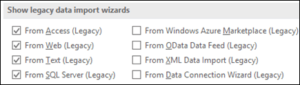
Close the workbook and then reopen it to see the activate the wizards
Select Data > Get Data > Legacy Wizards, and then select the wizard you want.
You can disable the wizards by repeating steps 1 through 3, but clearing the check boxes described in step 2.
Источник
Text Import Wizard
Although you can’t export to Excel directly from a text file or Word document, you can use the Text Import Wizard in Excel to import data from a text file into a worksheet. The Text Import Wizard examines the text file that you are importing and helps you ensure that the data is imported in the way that you want.
Note: The Text Import Wizard is a legacy feature that continues to be supported for back-compatibility. As an alternative, you can import a text file by connecting to it with Power Query.
Go to the Data tab > Get External Data > From Text. Then, in the Import Text File dialog box, double-click the text file that you want to import, and the Text Import Wizard dialog will open.
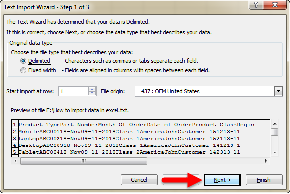
Step 1 of 3
Original data type If items in the text file are separated by tabs, colons, semicolons, spaces, or other characters, select Delimited. If all of the items in each column are the same length, select Fixed width.
Start import at row Type or select a row number to specify the first row of the data that you want to import.
File origin Select the character set that is used in the text file. In most cases, you can leave this setting at its default. If you know that the text file was created by using a different character set than the character set that you are using on your computer, you should change this setting to match that character set. For example, if your computer is set to use character set 1251 (Cyrillic, Windows), but you know that the file was produced by using character set 1252 (Western European, Windows), you should set File Origin to 1252.
Preview of file This box displays the text as it will appear when it is separated into columns on the worksheet.
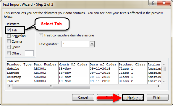
Step 2 of 3 (Delimited data)
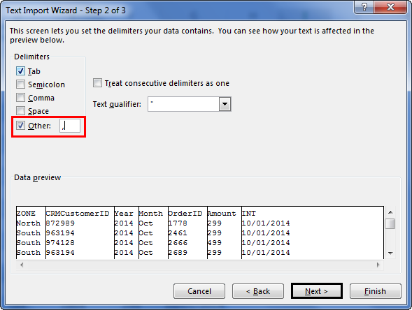
Delimiters Select the character that separates values in your text file. If the character is not listed, select the Other check box, and then type the character in the box that contains the cursor. These options are not available if your data type is Fixed width.
Treat consecutive delimiters as one Select this check box if your data contains a delimiter of more than one character between data fields or if your data contains multiple custom delimiters.
Text qualifier Select the character that encloses values in your text file. When Excel encounters the text qualifier character, all of the text that follows that character and precedes the next occurrence of that character is imported as one value, even if the text contains a delimiter character. For example, if the delimiter is a comma ( ,) and the text qualifier is a quotation mark ( «), «Dallas, Texas» is imported into one cell as Dallas, Texas. If no character or the apostrophe (‘) is specified as the text qualifier, «Dallas, Texas» is imported into two adjacent cells as «Dallas and Texas».
If the delimiter character occurs between text qualifiers, Excel omits the qualifiers in the imported value. If no delimiter character occurs between text qualifiers, Excel includes the qualifier character in the imported value. Hence, «Dallas Texas» (using the quotation mark text qualifier) is imported into one cell as «Dallas Texas».
Data preview Review the text in this box to verify that the text will be separated into columns on the worksheet as you want it.
Step 2 of 3 (Fixed width data)
Data preview Set field widths in this section. Click the preview window to set a column break, which is represented by a vertical line. Double-click a column break to remove it, or drag a column break to move it.
Step 3 of 3
Click the Advanced button to do one or more of the following:
Specify the type of decimal and thousands separators that are used in the text file. When the data is imported into Excel, the separators will match those that are specified for your location in Regional and Language Options or Regional Settings (Windows Control Panel).
Specify that one or more numeric values may contain a trailing minus sign.
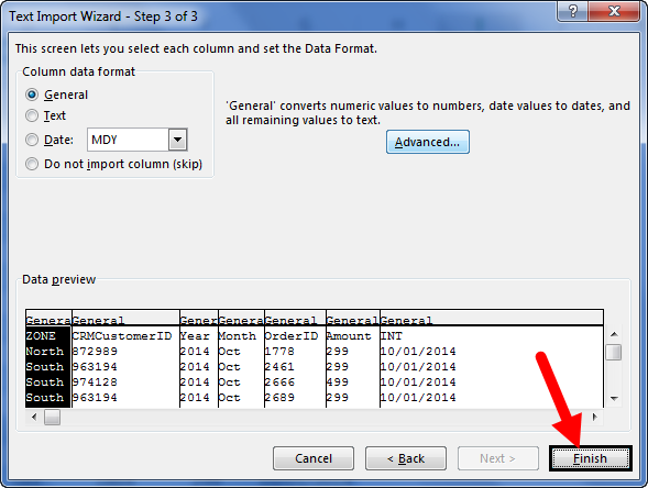
Column data format Click the data format of the column that is selected in the Data preview section. If you do not want to import the selected column, click Do not import column (skip).
After you select a data format option for the selected column, the column heading under Data preview displays the format. If you select Date, select a date format in the Date box.
Choose the data format that closely matches the preview data so that Excel can convert the imported data correctly. For example:
To convert a column of all currency number characters to the Excel Currency format, select General.
To convert a column of all number characters to the Excel Text format, select Text.
To convert a column of all date characters, each date in the order of year, month, and day, to the Excel Date format, select Date, and then select the date type of YMD in the Date box.
Excel will import the column as General if the conversion could yield unintended results. For example:
If the column contains a mix of formats, such as alphabetical and numeric characters, Excel converts the column to General.
If, in a column of dates, each date is in the order of year, month, and date, and you select Date along with a date type of MDY, Excel converts the column to General format. A column that contains date characters must closely match an Excel built-in date or custom date formats.
If Excel does not convert a column to the format that you want, you can convert the data after you import it.
When you have selected the options you want, click Finish to open the Import Data dialog and choose where to place your data.
Import Data
Set these options to control how the data import process runs, including what data connection properties to use and what file and range to populate with the imported data.
The options under Select how you want to view this data in your workbook are only available if you have a Data Model prepared and select the option to add this import to that model (see the third item in this list).
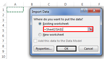
Specify a target workbook:
If you choose Existing Worksheet, click a cell in the sheet to place the first cell of imported data, or click and drag to select a range.
Choose New Worksheet to import into a new worksheet (starting at cell A1)
If you have a Data Model in place, click Add this data to the Data Model to include this import in the model. For more information, see Create a Data Model in Excel.
Note that selecting this option unlocks the options under Select how you want to view this data in your workbook.
Click Properties to set any External Data Range properties you want. For more information, see Manage external data ranges and their properties.
Click OK when you’re ready to finish importing your data.
Notes: The Text Import Wizard is a legacy feature, which may need to be enabled. If you haven’t already done so, then:
Click File > Options > Data.
Under Show legacy data import wizards, select From Text (Legacy).
Once enabled, go to the Data tab > Get & Transform Data > Get Data > Legacy Wizards > From Text (Legacy). Then, in the Import Text File dialog box, double-click the text file that you want to import, and the Text Import Wizard will open.
Step 1 of 3
Original data type If items in the text file are separated by tabs, colons, semicolons, spaces, or other characters, select Delimited. If all of the items in each column are the same length, select Fixed width.
Start import at row Type or select a row number to specify the first row of the data that you want to import.
File origin Select the character set that is used in the text file. In most cases, you can leave this setting at its default. If you know that the text file was created by using a different character set than the character set that you are using on your computer, you should change this setting to match that character set. For example, if your computer is set to use character set 1251 (Cyrillic, Windows), but you know that the file was produced by using character set 1252 (Western European, Windows), you should set File Origin to 1252.
Preview of file This box displays the text as it will appear when it is separated into columns on the worksheet.
Step 2 of 3 (Delimited data)
Delimiters Select the character that separates values in your text file. If the character is not listed, select the Other check box, and then type the character in the box that contains the cursor. These options are not available if your data type is Fixed width.
Treat consecutive delimiters as one Select this check box if your data contains a delimiter of more than one character between data fields or if your data contains multiple custom delimiters.
Text qualifier Select the character that encloses values in your text file. When Excel encounters the text qualifier character, all of the text that follows that character and precedes the next occurrence of that character is imported as one value, even if the text contains a delimiter character. For example, if the delimiter is a comma ( ,) and the text qualifier is a quotation mark ( «), «Dallas, Texas» is imported into one cell as Dallas, Texas. If no character or the apostrophe (‘) is specified as the text qualifier, «Dallas, Texas» is imported into two adjacent cells as «Dallas and Texas».
If the delimiter character occurs between text qualifiers, Excel omits the qualifiers in the imported value. If no delimiter character occurs between text qualifiers, Excel includes the qualifier character in the imported value. Hence, «Dallas Texas» (using the quotation mark text qualifier) is imported into one cell as «Dallas Texas».
Data preview Review the text in this box to verify that the text will be separated into columns on the worksheet as you want it.
Step 2 of 3 (Fixed width data)
Data preview Set field widths in this section. Click the preview window to set a column break, which is represented by a vertical line. Double-click a column break to remove it, or drag a column break to move it.
Step 3 of 3
Click the Advanced button to do one or more of the following:
Specify the type of decimal and thousands separators that are used in the text file. When the data is imported into Excel, the separators will match those that are specified for your location in Regional and Language Options or Regional Settings (Windows Control Panel).
Specify that one or more numeric values may contain a trailing minus sign.
Column data format Click the data format of the column that is selected in the Data preview section. If you do not want to import the selected column, click Do not import column (skip).
After you select a data format option for the selected column, the column heading under Data preview displays the format. If you select Date, select a date format in the Date box.
Choose the data format that closely matches the preview data so that Excel can convert the imported data correctly. For example:
To convert a column of all currency number characters to the Excel Currency format, select General.
To convert a column of all number characters to the Excel Text format, select Text.
To convert a column of all date characters, each date in the order of year, month, and day, to the Excel Date format, select Date, and then select the date type of YMD in the Date box.
Excel will import the column as General if the conversion could yield unintended results. For example:
If the column contains a mix of formats, such as alphabetical and numeric characters, Excel converts the column to General.
If, in a column of dates, each date is in the order of year, month, and date, and you select Date along with a date type of MDY, Excel converts the column to General format. A column that contains date characters must closely match an Excel built-in date or custom date formats.
If Excel does not convert a column to the format that you want, you can convert the data after you import it.
When you have selected the options you want, click Finish to open the Import Data dialog and choose where to place your data.
Import Data
Set these options to control how the data import process runs, including what data connection properties to use and what file and range to populate with the imported data.
The options under Select how you want to view this data in your workbook are only available if you have a Data Model prepared and select the option to add this import to that model (see the third item in this list).
Specify a target workbook:
If you choose Existing Worksheet, click a cell in the sheet to place the first cell of imported data, or click and drag to select a range.
Choose New Worksheet to import into a new worksheet (starting at cell A1)
If you have a Data Model in place, click Add this data to the Data Model to include this import in the model. For more information, see Create a Data Model in Excel.
Note that selecting this option unlocks the options under Select how you want to view this data in your workbook.
Click Properties to set any External Data Range properties you want. For more information, see Manage external data ranges and their properties.
Click OK when you’re ready to finish importing your data.
Note: If your data is in a Word document, you must first save it as a text file. Click File > Save As, and choose Plain Text (.txt) as the file type.
Need more help?
You can always ask an expert in the Excel Tech Community or get support in the Answers community.
Источник
Excel Import Data (Table of Contents)
- Import Data In Excel
- How To Import Data In Excel?
Import Data In Excel
Microsoft has provided some functions that can be used to import the data from different sources and connect them with excel. We can import the data from different sources such as from Access, Web, Text, SQL Server or any other database. We can connect Microsoft Excel with many sources and import the data in many ways.
How To Import Data In Excel?
Let’s see how to import data in Excel by using some examples:
You can download this Import Data in Excel Template here – Import Data in Excel Template
Import Data In Excel – Example #1
Many times we faced a situation where we need to extract or import the data from other sources. And in Excel, we can use the function Get External Data to import the required fields to work from different sources.
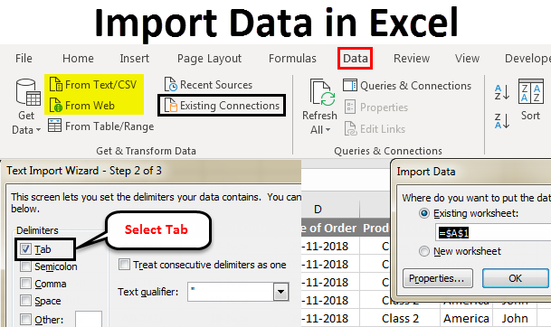
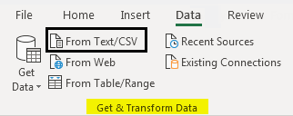
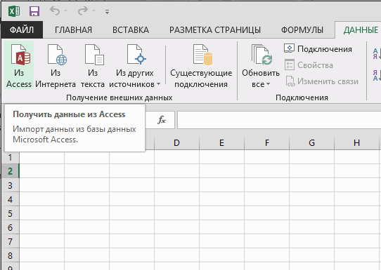
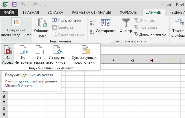
We can extract the data in excel by going in the Data menu tab, under getting and Transform data, select any required source as shown below.
Those options are shown in the below screenshot.
There are many different ways to import data in excel.
- From Text/CSV: Text files whose data can be separated with a tab or excel columns.
- From Web: Any website whose data can be converted to excel tables.
- From Table/Range: Create a new query linked to the selected Excel table or named range.
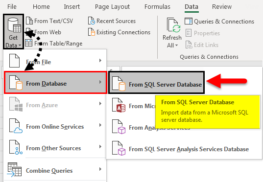
Above mentioned ways of importing the data are majorly used. There are some other ways also, as shown in the below screenshot. For that, click on From SQL Server Database under From Database section. Once we do that, we will get a drop-down list of all the other sources from where we can import the data.
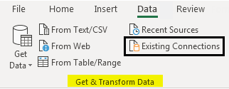
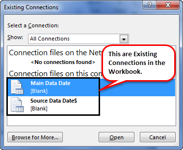
Once we import the data from any server or database, the connection gets established permanently till we remove it manually. And in the future, we can import the data from previously established and connected sources to save time. For this, go to the Data menu tab; under Get & Transform Data, select Existing Connections as shown below.
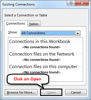
Once we click on it, we will get a list of all existing connections which we link with our computer or excel or network, as shown below. From that list, select the required connection point and click on Open to access that database.
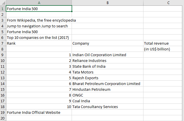
Now let’s import some data from any website. For that, we must have the link to that website from where we need to import the data. Here, for example, we have considered the link of Wikipedia as given below.
Link: https://en.wikipedia.org/wiki/Fortune_India_500
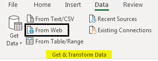
Now, go to the Data menu; under Get & Transform Data section, select From Web as shown below.
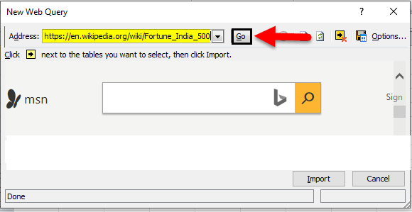
Once we do that, we will get a Web Query box. There at the address tab, copy and paste the link and click on Go as shown below.
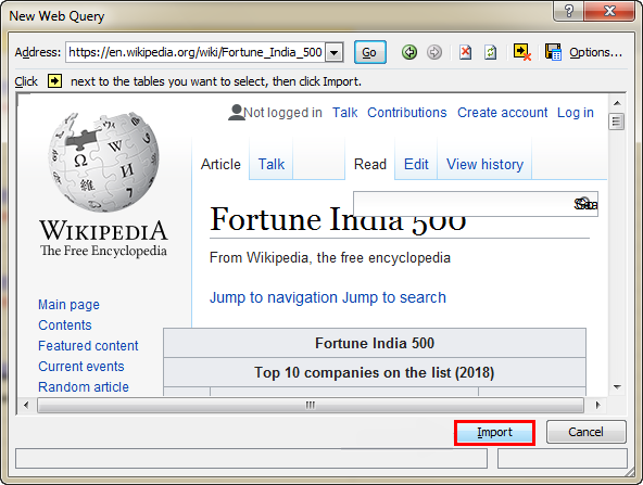
It will then take us to the web page of that link, as shown below. Now click on the Import button to import the data.
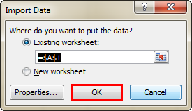
The Import Data box will appear, asking for a reference cell or sheet to import the data. Here we have select cell A1 as shown below. And click on, OK.
Then the query will run, and it will fetch the data from the provided link as shown below.
Import Data In Excel – Example #2
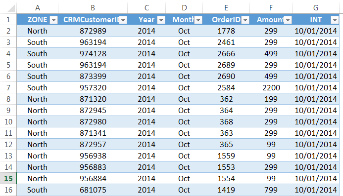
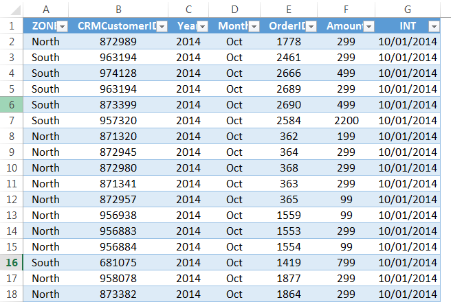
Let’s see another way of importing the data. For this, we have some sample data in Notepad (or Text) file, as shown below. As we can see, the data has spaces between the lines like columns in excel has.
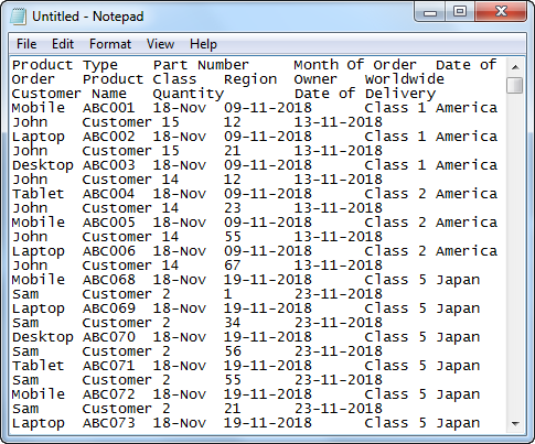
Importing such data is easy as it is already separated with spaces. Now to import the data in the text file, go to the Data menu tab, under the getting and Transform data section, select From Text option as shown below.
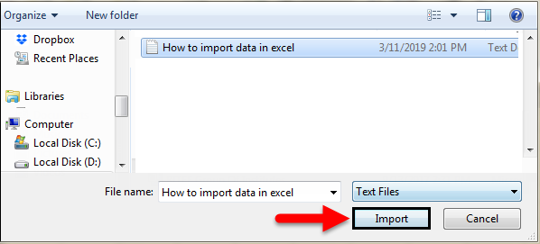
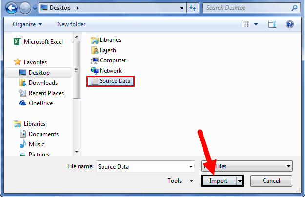
After that, we will get a box where it will ask us to browse the file. Search and select the file and click on the Import button to process further.
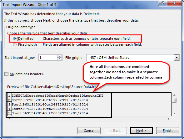
Just after that, a text import wizard will appear, which will ask us to delimit or separate the text. Select the Delimited option for a proper way to separate the data into columns or select the Fixed Width option to do it manually. Here we have selected Delimited as shown below.
Here we have delimited the text with Tab as shown below. Now click on Next to complete the process.
Now select the way we want to import the data. Here we have selected cell A1 for the reference point and click on OK.
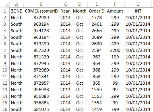
We will see our data imported to excel from the selected file.
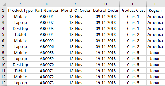
Like this, we can import the data from different sources or databases to excel to work on them.
Pros of Importing Data in Excel
- By importing the data from any other sources, we can link different tables, files, columns, or sections and get the data we require.
- It saves time by manually copying and pasting the heavy data from one source to excel.
- We also avoid unnecessary crashing or handing of files if the data is huge.
Cons of Importing Data in Excel
- Sometimes processing time is huge.
Things to Remember
- Make sure you are connected to a good internet connection when you are importing data from SQL Servers or similar databases.
- Do not do anything while data is being imported from the source files or database. It may crash the opened files.
- Always protect the previously established connection with a password.
Recommended Articles
This has been a guide to Importing Data in Excel. Here we discussed how to import data in excel along with practical examples and a downloadable excel template. You can also go through our other suggested articles to learn more –
- Auto Numbering in excel
- Watermark in Excel
- Enable Macros in excel
- Excel Uppercase Function
How to Import Data in Excel?
Importing the data from another file or another source file is often required in Excel. For example, sometimes people need data directly from very complicated servers, and sometimes we may need to import data from a text file or even from an Excel workbook.
If you are new to Excel data importing, then in this article, we will take a tour of importing data from text files, different Excel workbooks, and MS Access. Follow this article to learn the process involved in importing the data.
Table of contents
- How to Import Data in Excel?
- #1 – Import Data from Another Excel Workbook
- #2 – Import Data from MS Access to Excel
- #3 – Import Data from Text File to Excel
- Things to Remember
- Recommended Articles
#1 – Import Data from Another Excel Workbook
You can download this Import Data Excel Template here – Import Data Excel Template
Let us start.
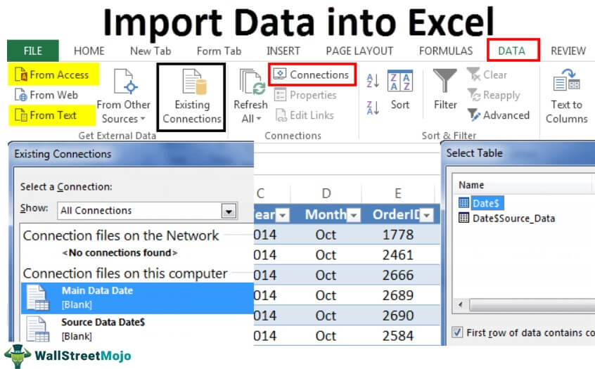
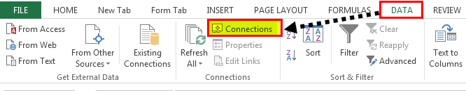
- First, we must go to the DATA tab. Then, under the DATA tab, click on Connections.

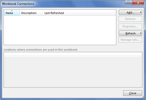
- As soon as we click on Connections, we may see the below window separately.

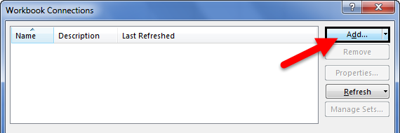
- Now, click on Add.

- It will open up a new window. In the below window, select All Connections.

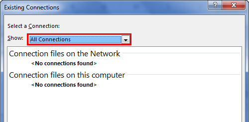
- If there are any connections in this workbook, it will show what those connections are here.

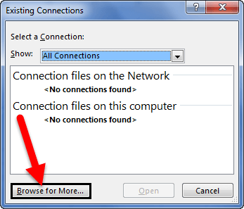
- Since we are connecting to a new workbook, click on Browse for more.

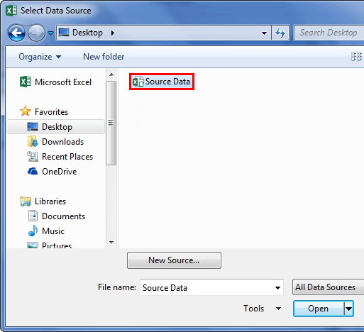
- In the below window, browse the file location. Then, click on Open.

- After clicking on Open, it shows the below window.

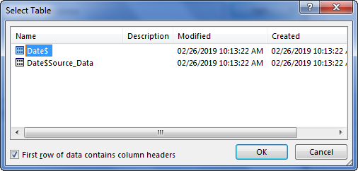
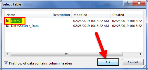
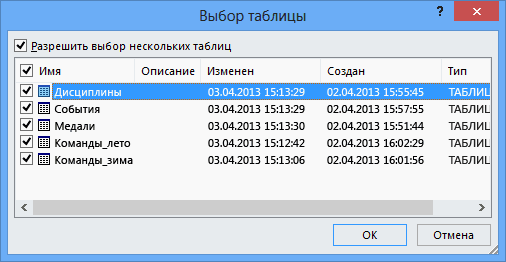
- Here, we need to select the required table to be imported to this workbook. Select the table and click on OK.
After clicking on OK, close the Workbook Connection window.
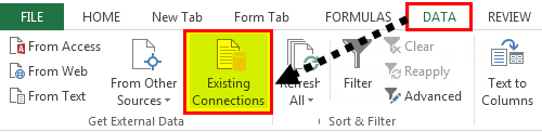
- Then, go to Existing Connections under the DATA tab.

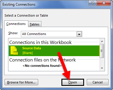
- Here, we will see all the existing connections. Select the connection we have just made and click on Open.

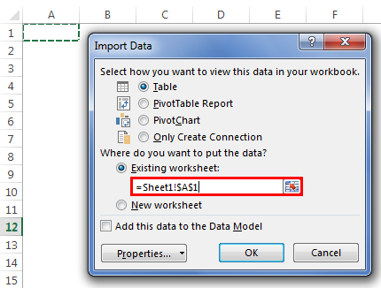
- Once we click on Open, it will ask us where to import the data. First, we need to select the cell reference here. Then, click on the OK button.

- It will import the data from the selected or connected workbook.

Like this, we can connect to the other workbook and import the data.
#2 – Import Data from MS Access to Excel
MS Access is the main platform to store the data safely. We can import the data directly from the MS Access File itself whenever the data is required.
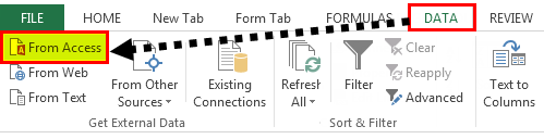
Step 1: Go to the “DATA” ribbon in excelThe ribbon is an element of the UI (User Interface) which is seen as a strip that consists of buttons or tabs; it is available at the top of the excel sheet. This option was first introduced in the Microsoft Excel 2007.read more and select “From Access.“
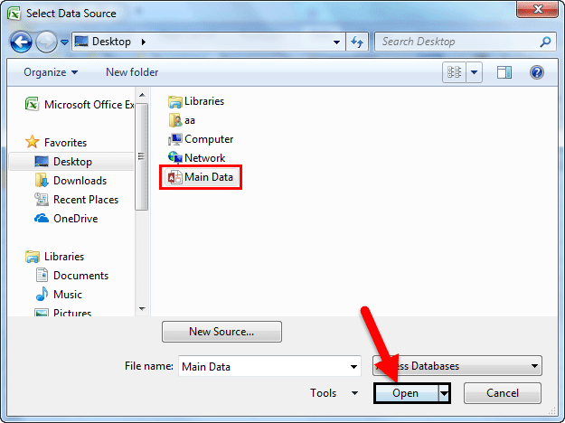
Step 2: Now, it will ask us to locate the desired file. Select the desired file path. Then, click on “Open.”
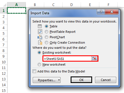
Step 3: Now, it will ask us to select the desired destination cell where we want to import the data. Then, click on “OK.”
Step 4: It will import the data from access to the A1 cell in Excel.
#3 – Import Data from Text File to Excel
In almost all the corporations, whenever we ask for the data from the IT team, they will write a query and get the file in TEXT format. But unfortunately, TEXT file data is not the ready format to use in Excel; we need to make some modifications to work on it.
Step 1: Go to the “DATA” tab and click on “From Text.”

Step 2: Now, it will ask us to choose the file location on the computer or laptop. Select the targeted file, then click on “Import.”
Step 3: It will open up a “Text Import Wizard.”
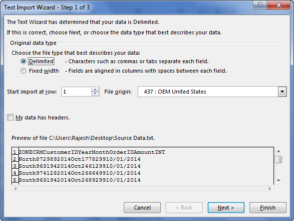
Step 4: By selecting the “Delimited,” click on “Next.”
Step 5: In the next window, select the other and mention comma (,) because, in the text file, each column is separated by a comma (,). Then click on “Next.”
Step 6: In the next window, click on “Finish.”
Step 7: Now, it will ask us to select the desired destination cell where we want to import the data. Select the cell and click on “OK.”
Step 8: It will import the data from the text file to the A1 cell in Excel.
Things to Remember
- If there are many tables, we must specify which table data we need to import.
- If we want the data in the current worksheet, we need to select the desired cell. Else, if we need data in a new worksheet, we must choose the new worksheet as the option.
- We need to separate the column in the TEXT file by identifying the common column separators.
Recommended Articles
This article is a guide to Import Data in Excel. Here, we discuss how to import data from 1) Excel Workbook, 2) MS Access, 3) Text File, practical examples, and a downloadable Excel template. You may learn more about Excel from the following articles: –
- KPI Dashboard in Excel
- Insert Image in Excel Cell
- How to Insert New Worksheet In Excel?
- Create a Dashboard in Excel
- Page Numbers in Excel
Excel is a preferred option for many people when it comes to processing data. Any calculations can be done with the help of Excel formulas, while Excel macros leave much space for all kinds of automatization.
But not all the data is stored in the form of spreadsheets. There are plenty of systems and tools for data collection and management. Thankfully, Excel is extremely flexible in terms of data importing. This article will explain how you can export data from the most popular sources to Excel.
Importing web data to Excel
Who needs to import data from the web to Excel
It’s not a secret that the internet is made of data. Thanks to the development of broadband networks and wireless technologies, all that data is available at your fingertips at any moment.
But sometimes, you may need to go beyond just reading the information. For example, when you are working on research and want to analyze large amounts of data. In this case, it would be helpful to import web data into specialized software, such as Excel.
How to import data from HTML to Excel
Of course, the simplest way to import data from a website to Excel is to copy-paste it from an HTML page by using a web browser. Sometimes that works pretty well; the simpler, the better. But what if the required data is on hundreds of pages? Or maybe, you don’t need all the information, but only specific fields. In such cases, the simple method will consume an unreasonable amount of time.
Excel has a built-in feature for scraping tables from web pages. To import data from a web source:
- On the Data tab, select New Query > From Other Sources > From Web:
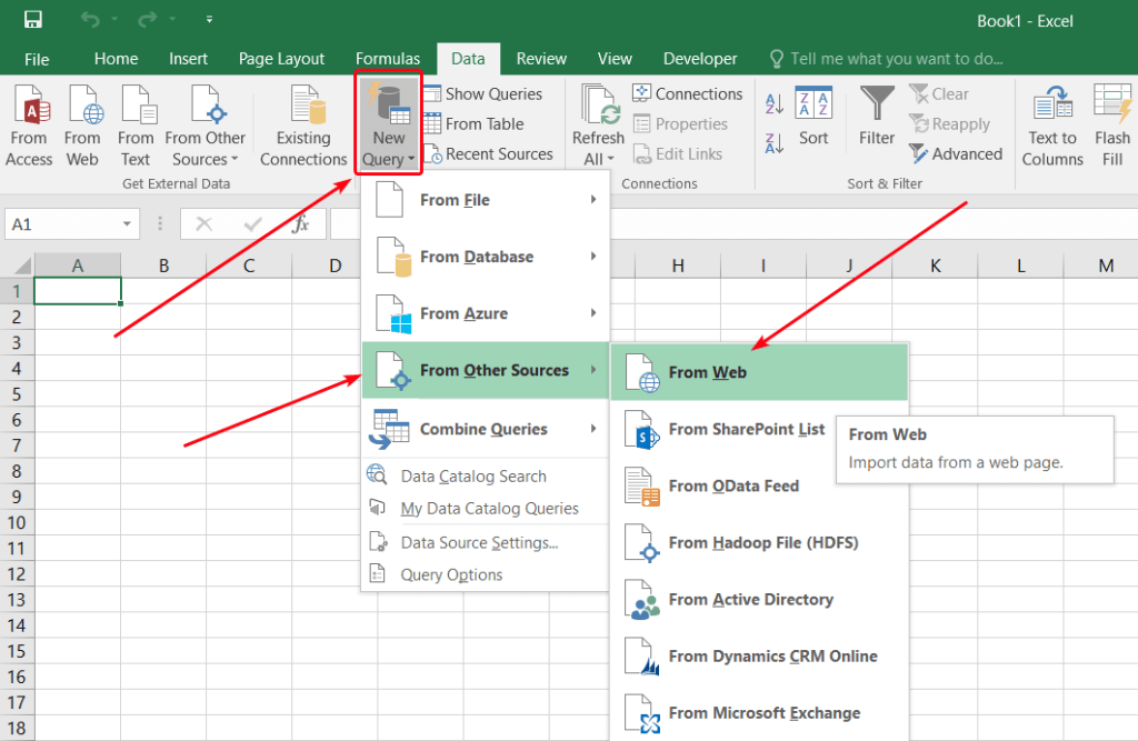
- Enter the web page URL and click OK:

Excel will look for tables on the page.
- In the Navigator window that opens, select the table that you want to import:

Use the Select multiple items checkbox if you want to import several tables. Click Load when you are ready to start the import.
- Excel will insert the imported table into the current worksheet. You can refresh data by clicking the refresh button in the Workbook Queries task pane:

How to automatically import live data into Excel
Data is relevant as long as it’s fresh. If you need to update the information frequently to keep it up-to-date, manual data import will bring nothing but pain.
Thankfully, many websites provide REST API for accessing their data. Sometimes you have to pay for API access, sometimes it’s free. You need to make a request to get the data. The details on making requests can be found in the API reference of the data provider. API responses usually contain data in JSON format. There are free services that allow you to import JSON data to Excel. The best ones will even make API requests for you. Let’s see how you can use Coupler.io for such tasks.
Coupler.io is a data integration solution for importing data into Excel from different apps. You can load records from Shopify, HubSpot, Pipedrive, and many other sources. In addition to Excel, you can use Google Sheets or BigQuery as a destination for your data.
- Sign in to Coupler.io with your Microsoft account.
- Go to Importers and click Add new importer.
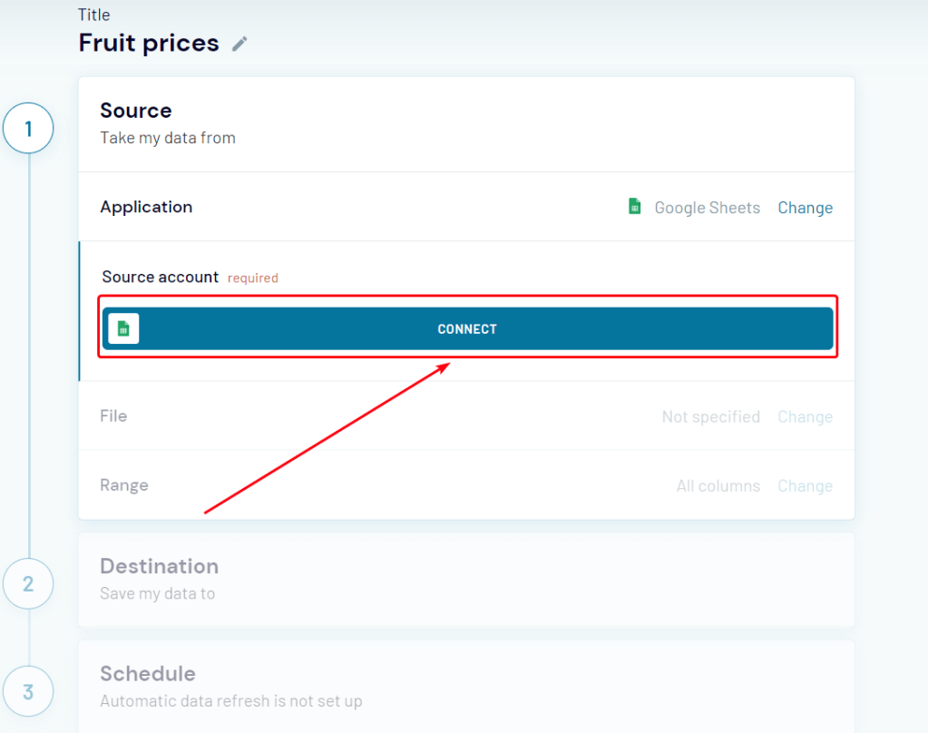
- Select JSON as Source, and provide the request URL with your API key (if required):

Refer to the data provider documentation for details on available requests and how you can obtain an API key.
- Specify API call parameters, as described in the API documentation. The only required parameter is HTTP method, which will be ‘GET’ in most cases.
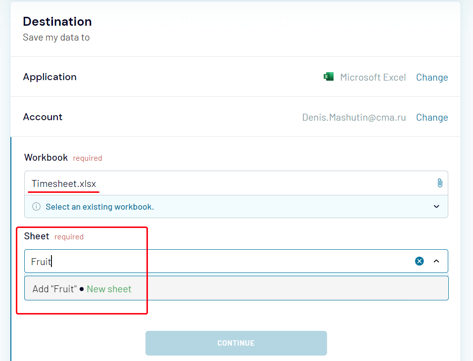
- In Destination, select Microsoft Excel:

- Connect to your Microsoft Office account, and then select an existing workbook for import. You can specify an existing sheet or create a new one by typing its name:

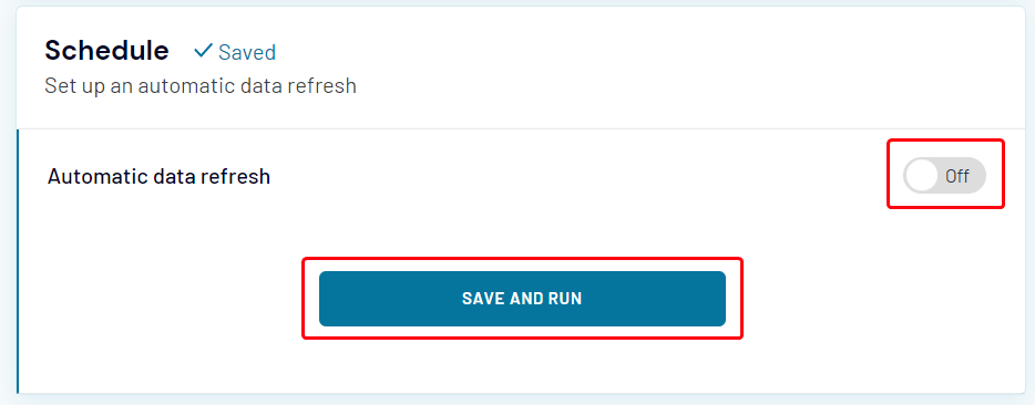
- Toggle the Automatic data refresh switch to set up the schedule for automatic data updates. When you are done with settings, click Save and Run:

Synchronizing the spreadsheets
How to sync data between Excel files
If you want to transfer data from one Excel workbook to another, copy-pasting is a good option. But that will not work if you want to keep the data up-to-date with the other file. There are several ways to sync data between Excel files.
You can use formulas for that. To fill a cell with data from another Excel workbook:
- Make sure that the other workbook is open.
- Select the cell to sync, then click the Formula Bar and type
=.

- Switch to the other workbook, click the cell that you want to import data from, and press Enter.
Excel will switch you back to the first workbook and fill the cell with the synced data. If the content of the cell in the other workbook changes, the synced cell will be updated.
If you see #REF! in the synced cell, it means that the other workbook is not open. Open it to enable data synchronization. Try another method if you are not comfortable with the formula bar.
- In the source file, i.e. the workbook that you want to import data from, select the cell, and then click Copy or press
Ctrl-C:

- Switch to the target workbook, select the cell, and then select Paste > Other Paste Options > Paste Link.
The formula for that cell will be filled with the link to the source cell in the other workbook.
There are many other options for syncing Excel data that you can learn in our guide on linking Excel files.
Besides the standard Excel features, there are online tools that allow you to import data from Excel to Excel, and let you synchronize your data in a more flexible way.
How to import data from Google Sheets to Excel
Google Sheets is almost as powerful as Excel in terms of data processing. But certain very important features are still available only in Excel. If you need these functions, you can transfer your data in several ways.
Import data from Google Sheets to Excel automatically
First of all, try using Coupler.io. It is an online tool that can import data from Google Sheets to Excel.
- Sign in to your Coupler.io account and click Add New in the Importers section.
- Select Google Sheets as Source, click Connect, and sign in to your Google account:
- Select the workbook and the sheet that you would like to export data from:

- Select the range of cells, or skip this step to export all the data.
- In Destination, select Microsoft Excel, click Continue, and then sign in to your Microsoft account.
- Select an existing workbook and the worksheet. If you want to create a new worksheet, just type its name:
- Specify the cell address or keep the default ‘A1’ value.
- Specify the import mode. The default option is ‘Replace’.
- Now you can click Save and Run to start the import immediately.
Or you can toggle Automatic data refresh to configure automatic data updates:
Import data from Google Sheets to Excel as HTML
The second option is to use the built-in data import feature of Excel:
- In your Google spreadsheet, go to File > Share > Publish to web:
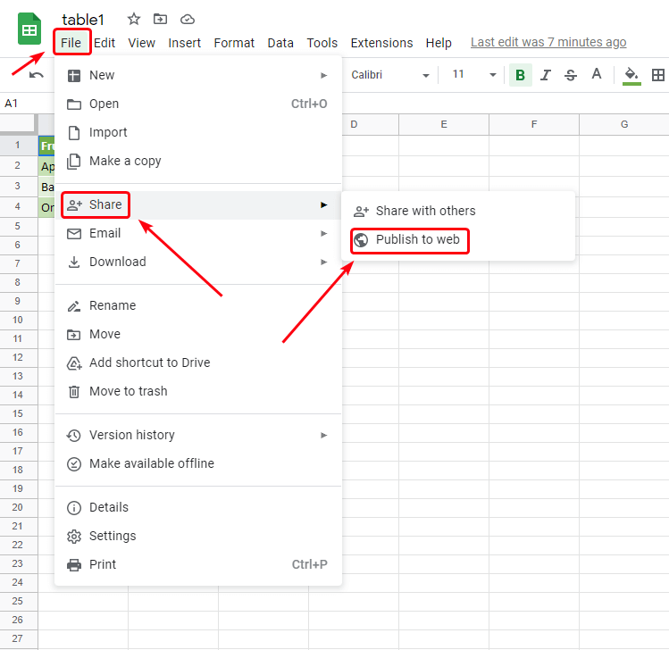
- Select the sheet that contains the table, and specify Comma-separated values (.csv).
If you want the data in Excel to be updated when the Google sheet is changed, select the Automatically republish when changes are made checkbox:

- Press
Ctrl-Cto copy the link. - Go to your Excel workbook and perform the steps described in the section about importing data from HTML above.
If you choose the second option, keep in mind that your data will become accessible by others. If the information is confidential or sensitive, using Coupler.io is preferred.
Importing data from other sources
How to import data from SQL server to Excel
If your data is stored in databases at an SQL server, the simplest way to make it accessible to a wide spectrum of users is to export it to Excel. You can use the native Excel query function.
- In the Data tab, select New Query > From Database > From SQL Server Database:
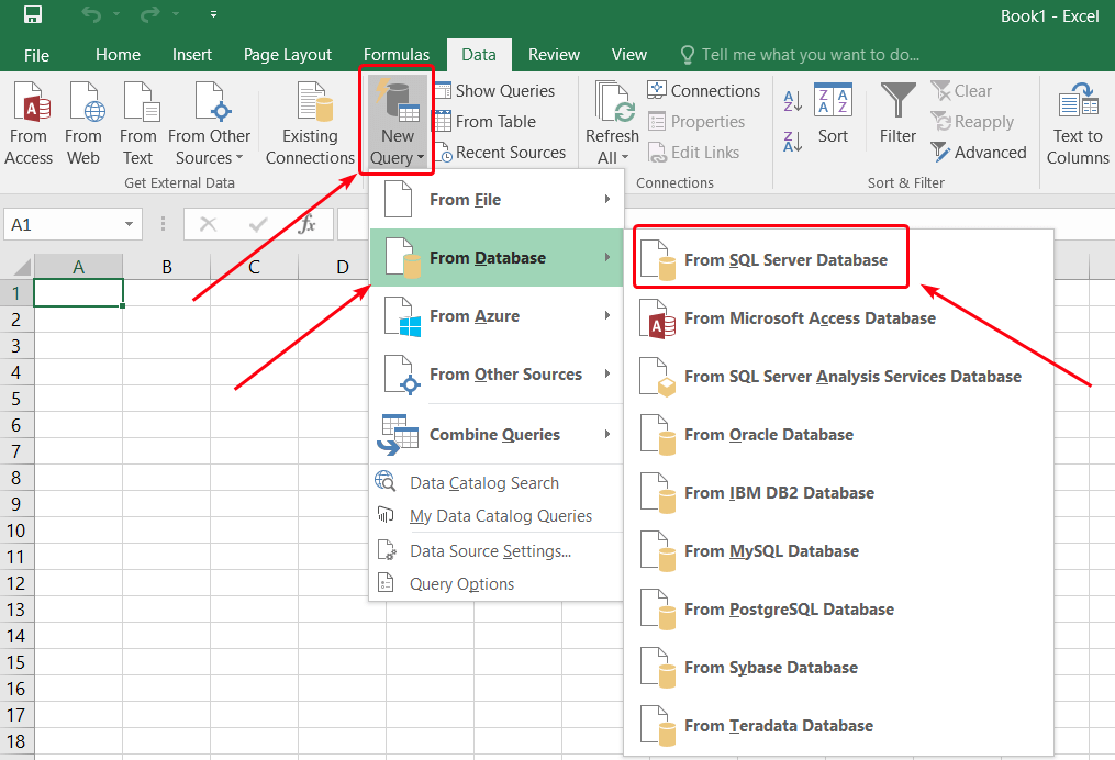
- Specify the name of the server and the database (or you will be able to specify it later):

You can also provide an SQL statement to narrow the range of exported data.
- Choose to use your current window credentials to access the database, or provide the username and the password. Click Connect.
- In the next window, select the database and tables that you want to export.
- Select the name for the new data connection file, and then click Finish.
- In the next window, you can select where to insert the imported data. Select Existing worksheet and provide the cell address, if needed.
The data will be imported and pasted into the worksheet.
If you use SQL Server Management Studio (SSMS), there is a feature for exporting data to various destinations, including Excel spreadsheets.
- In Object Explorer, right-click the database with the source data, and then select Tasks > Export Data.
- In the SQL Server Import and Export Wizard window that opens, click Next.
- Select SQL Server Native Client 11.0 in the Data source drop-down box.
- Select Use Windows Authentication in the Authentication area, and then click Next.
- In the Choose a destination window, specify Microsoft Excel as the destination, browse to the target file in the Excel file path, and select the output file format.
- In the next window, you can choose to write a query for data export. If you want to copy the tables without changes, just click Next.
- The list of tables available for export will be displayed. Select the tables that you want to export. In the Destination column, you can specify the name of the worksheet for each table.
- In the Save and Run Package window, select Run immediately and click Next.
- Make sure that all parameters are correct, and then click Finish.
The selected data will be exported to the Excel workbook. When the wizard finishes all the tasks, click Close.
How to import data from a text file to Excel
The tables can also be stored in plain text. Such files are similar to regular text files with the only exception that commas have a special function there — they separate cells from each other. The format is called CSV — comma-separated values.
Excel can open .csv files directly. The content of such a file will be rendered as a table. If you edit a CSV file in Excel and then try to save it, you will see the following warning:

Click Yes if you want to continue using this file as CSV in the future. If you click No, the Save as dialogue will be opened, where you will be able to select the format and the destination for the file.
There are other delimiters that can be used to store tables in text format: tabs, pipes (‘|’), spaces, semicolons, etc. To open such files with Excel, instead of trying to open them directly, use the Power Query function.
- Go to Data > New Query > From File > From Text.
- Select the text file and click Import.
- The Query Editor window will open. Make sure that the table looks good and click Close & Load:

The imported table will be inserted into your current worksheet.
How to import data to Excel from PDF
If your tables are in PDF, but you want them in Excel, you can try to import them.
- Go to the Data tab, and then select New Query > From File > From PDF.
- Select the tables that you want to import in the Navigator window, and then click Load.
The tables will be extracted from PDF and pasted into your Excel workbook. If you don’t have the From PDF option on the menu, you can use the following workaround to import data from PDF into Excel:
- Copy the table text in the PDF file by selecting it and pressing
Ctrl-C. - Open Microsoft Word and press
Ctrl-V. - Check if Word managed to render the text data correctly:
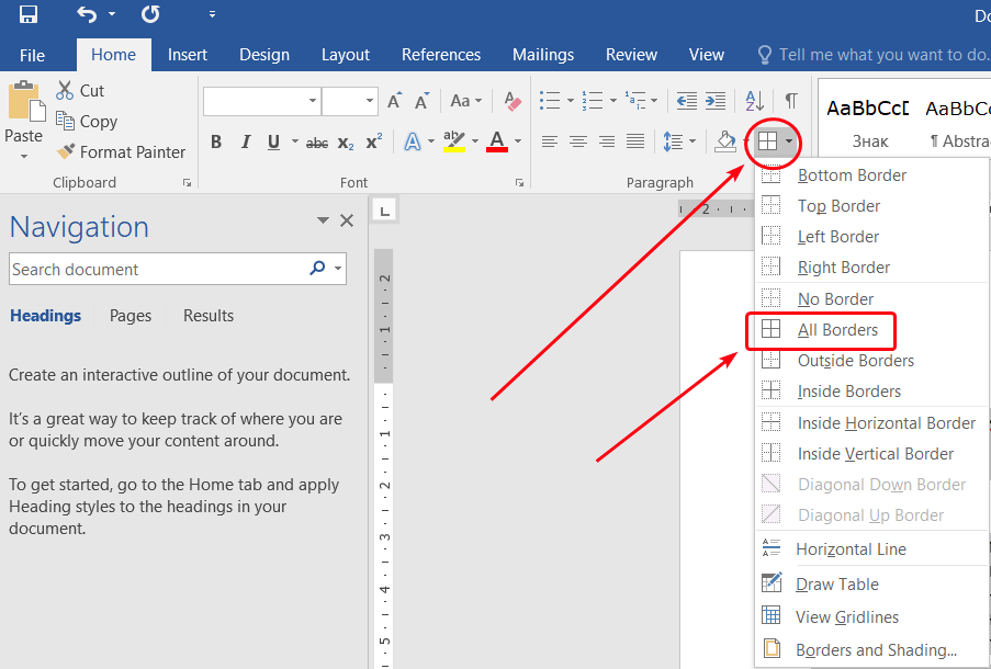
- Press
Ctrl-Ato select everything. - On the Home tab, click the table menu, and then select All borders:
- Press
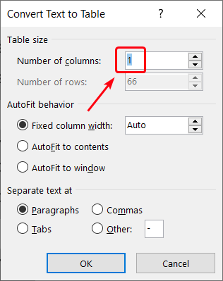
- If the table looks good, proceed to the final step. Otherwise, go to the Insert tab, and then select Table > Convert Text to Table:

- Specify the number of columns in the original table, and then click OK:
- Copy the entire table, go to Excel, and press
Ctrl-V.
The table will be inserted into the current worksheet. If you opt for this workaround, no automatic data synchronization will be available.
Discover many other sources for importing data to Excel
Excel provides you with many powerful features for data processing. You can bring virtually any data to Excel by importing it from various sources. If you didn’t find a good solution in this article, discover other Microsoft Excel integrations to pick what fits your needs best.
-

Lead Analytics Engineer at Railsware and Coupler.io. I make data accessible and useful for everyone in a team. During the last 7 years, I built dashboards, analyzed user journeys, and even caught criminals 🕵🏿♀️ Besides data, I also like doing yoga, cooking, and hiking 🤗

Back to Blog
Focus on your business
goals while we take care of your data!
Try Coupler.io
Skip to content
![]()
Microsoft quietly replaced the comfortable Text Import Wizard from Excel and replaced it with the “Get & Transform” tools. The “Get & Transform” tools offer a lot of options and are very powerful. Unfortunately, they are quite complicated to use. Here is what you should now.
In a hurry? Click on “File” –> “Options” –> “Data” and set the corresponding checkmarks for reactivating the “Text Import Wizard” in Excel. Start the text import by clicking on “Data” –>”Get Data” –> “Legacy Wizards” –> “From Text (Legacy)”.
Introduction
In Excel 365 (only) 2016 (since version 1704) the “Text Import Wizard” was removed. It was replaced by the powerful “Get & Transform” tools. The “Get & Transform” tools also provide a function to import text and CSV files into Excel.
You have the following two options:
- Luckily, the comfortably “Text Import Wizard” still exists. You can re-activate and use it for importing text and csv files into Excel.
- Use the import function of the “Get & Transform” tools.
Restore the “Text Import Wizard”
The good news: You can easily restore the “Text Import Wizard”. Unfortunately, the option for re-activating them is hidden.
Follow these steps:
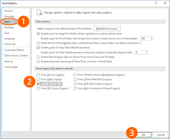
- Click on File and then on “Options”. Go to “Data” on the left-hand side.
- In the lower section of the window you can select the wizard you’d like to restore. For only importing text- or csv-files, select “From Text (Legacy)”. Feel free to also activate the corresponding wizard for importing Access files, files from web, from SQL servers and so on.
- Confirm with OK.
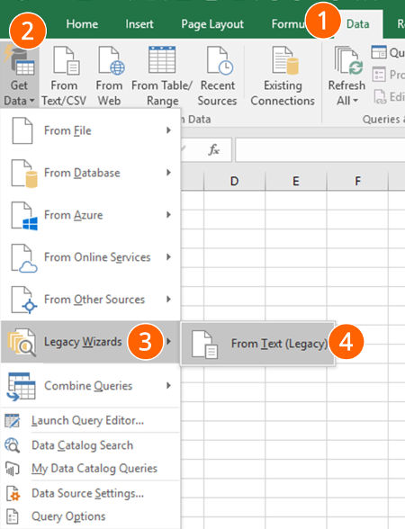
Now, you can find the so-called “Legacy Wizards” in the “Get Data” drop-down menu. In order to use them, follow these steps:
- Go to the “Data” ribbon.
- Click on “Get Data” on the left-hand side.
- Next, go to “Legacy Wizards”.
- Click on “From Text (Legacy)”.
How to use the “Text Import Wizard”
The steps for using the “Text Import Wizard” in Excel are shown in the screenshots.
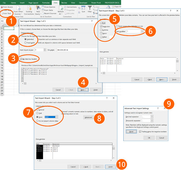
- Go to the “Data” ribbon and click on “From Text”. If you have a recent Excel version and there is no button called “From Text” (but instead “From Text/CSV”), click on “Get Data”, then on “Legacy Wizards” and then on “From Text (Legacy)”. Please refer to the paragraph above if this option is missing.
- Select how you want to define the columns: Either with a character as a separator or with a fixed width.
- If the first row contains headers, check the corresponding box.
- Continue with “Next >”.
- Select the delimiter. This is the character dividing the data into columns, for example “Tab”, “Semicolon” or “Comma”.
- Usually text fields use quotation marks marking the beginning and end of a text field.
- For each column, you can choose the data format. For dates, you could define the order of days, months and years.
- Click on “Advanced”…
- …for defining decimals and thousands separators.
- Finalize the import by clicking on “Finish”.
Import text and csv files with the “Get & Transform” tools
Importing text files in Excel with the “Get & Transform” tools requires many steps. Please refer to the numbers on the screenshots:
- Click on “From Text/CSV” on the “Data” ribbon in order to start the import process.
- Choose the delimiter (e.g. semi-colon, comma etc.). Here you can also switch to “Fixed Width”. If you want to separate your import data with the “Fixed Width” option, you have to type the numbers of characters, after which you want to data to be divided.
- For further options (e.g. switching thousands- and decimal separators) click on “Edit”.
- If you data is not represented correctly, delete the automatically created step “Changed Type”.
- Change the date format: Right-click on a column that contains a date. Alternatively click on the small “ABC” symbol in the top left corner of the column heading.
- Move the mouse to “Change Type”.
- Click on “Using Locale…”.
- Select “Date”.
- Select the locale format for dates. In this example, the German date format is used.
- Confirm with OK. Repeat the steps 5 to 10 for each date column.
Recommendation: Select several date columns at the same time by pressing and holding the Ctrl key while selecting the columns. - Change the decimal and thousand separators: Right-click again on a column with decimal numbers.
- Move the mouse to “Change Type”.
- Click on “Using Local…”.
- Choose “Decimal Number”.
- Select the local number format. Please refer to this article for a list of local number formats.
- Confirm with “OK”.
- Last step: Insert the data into a worksheet. In order to achieve this, click on “Close & Load” in the top-left corner.

Henrik Schiffner is a freelance business consultant and software developer. He lives and works in Hamburg, Germany. Besides being an Excel enthusiast he loves photography and sports.
We use cookies on our website to give you the most relevant experience by remembering your preferences and repeat visits. By clicking “Accept”, you consent to the use of ALL the cookies.
.
Excel can import and export many different file types aside from the standard .xslx format. If your data is shared between other programs, like a database, you may need to save data as a different file type or bring in files of a different file type.
Export Data
When you have data that needs to be transferred to another system, export it from Excel in a format that can be interpreted by other programs, such as a text or CSV file.
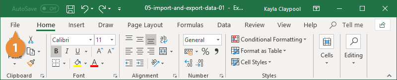
- Click the File tab.

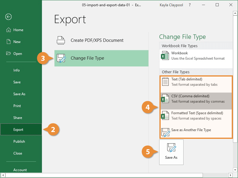
- At the left, click Export.
- Click the Change File Type.
- Under Other File Types, select a file type.
- Text (Tab delimited): The cell data will be separated by a tab.
- CSV (Comma delimited): The cell data will be separated by a comma.
- Formatted Text (space delimited): The cell data will be separated by a space.
- Save as Another File Type: Select a different file type when the Save As dialog box appears.
The file type you select will depend on what type of file is required by the program that will consume the exported data.
- Click Save As.

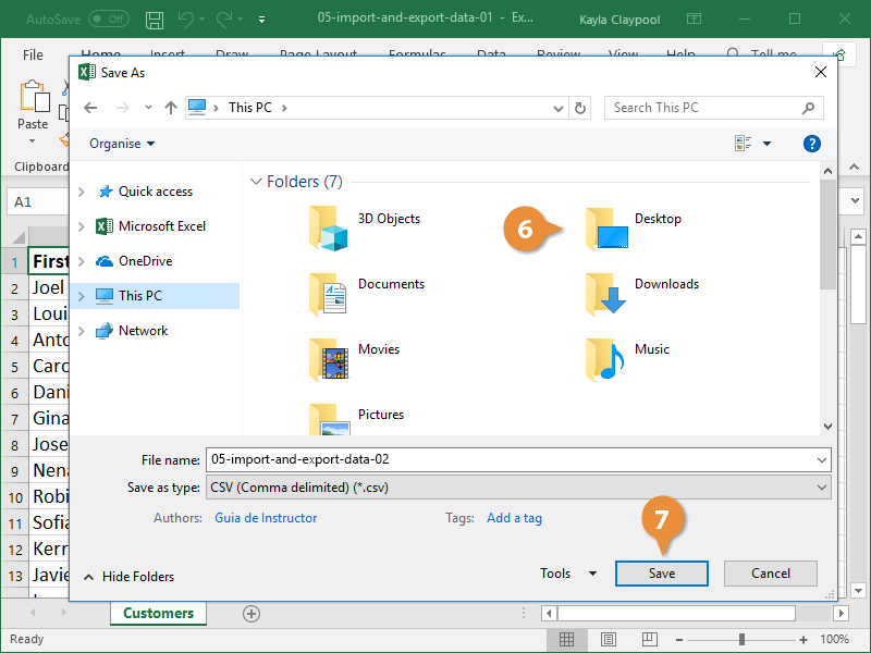
- Specify where you want to save the file.
- Click Save.
A dialog box appears stating that some of the workbook features may be lost.
- Click Yes.
Import Data
Excel can import data from external data sources including other files, databases, or web pages.
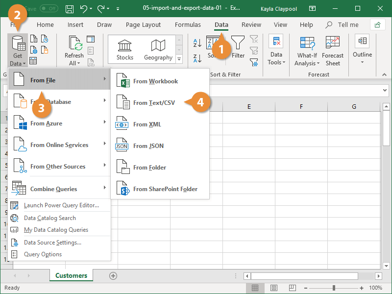
- Click the Data tab on the Ribbon..
- Click the Get Data button.
Some data sources may require special security access, and the connection process can often be very complex. Enlist the help of your organization’s technical support staff for assistance.
- Select From File.
- Select From Text/CSV.
If you have data to import from Access, the web, or another source, select one of those options in the Get External Data group instead.
- Select the file you want to import.
- Click Import.
If, while importing external data, a security notice appears saying that it is connecting to an external source that may not be safe, click OK.
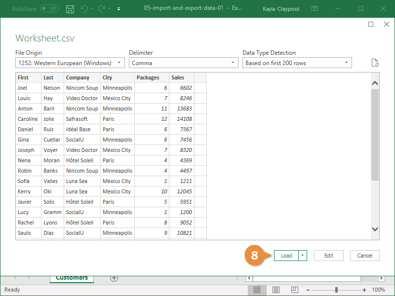
- Verify the preview looks correct.
Because we’ve specified the data is separated by commas, the delimiter is already set. If you need to change it, it can be done from this menu.
- Click Load.

FREE Quick Reference
Click to Download
Free to distribute with our compliments; we hope you will consider our paid training.
In the last section, you saw how to do a basic text import. The Text Import Wizard offers a lot of options to customize this type of import. You can specify how you’d your text data to be imported, minimizing the amount of cleanup that you need to do on the data.
In this section, we’ll use Ideal_Gas_Property_Data.txt as the data source. Go to Data > Get External Data > From Text, and open that file. The first window of the Text Import Wizard will open.
There are two main types of data files that you’ll import into Excel. Delimited files have a character separating the columns (i.e. a tab stop). Fixed width files have a specific number of characters in each column.
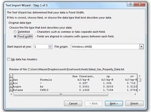
First, we’ll see how this data looks with the Delimited option. Choose it, then click Next.
Delimiters can be virtually any character. Tab, comma and space are the most common. The tab character is selected by default. However, in the preview window, there are no black lines separating the column – this tells us that Excel hasn’t found any tab delimiters. Unselect Tab, and choose Space. Now, black lines will appear between the columns:
Excel recognizes that the columns of data are separated by spaces. It automatically checks the box for “Treat consecutive delimiters as one.” In this text file, there are multiple spaces between the columns of data. If this box was not checked, each space would indicate a new column.
Click Next, then Finish. Choose a location on the worksheet to store the data and click OK.
Viewing the data in the spreadsheet exposes a flaw in selecting the space delimiting option. Gas names such as “carbon dioxide” and “carbon monoxide” are composed of two words separated by a space. Excel interprets this space as a column separator, so those rows have an extra column and all of the data is shifted:
Although we could manually clean up the data, those changes would be lost if the data were refreshed.
Instead, we’ll choose better options in the Text Import Wizard. Right-click on the data and select Edit Text Import.
Next, double-click on the file Ideal_Gas_Property_Data.txt.
This time, instead of the Delimited option, choose Fixed width. Click Next. Excel will automatically determine where the columns should be, and places break lines as separators between them. To move a break line, click and drag it to a new position.
You can also add or remove break lines. To add one, click at the top of the preview window, below the ruler (where the arrowheads are showing for the existing break lines). To delete one, double-click on it, or drag it away from the preview window.
Don’t worry about any excess spaces before or after an entry. Excel will clean those up. Just adjust the break lines so that each column includes all of the intended data. In this case, the defaults are fine. Click Next.
The third window of the Text Import Wizard contains options to set a data format for each column. The General format is appropriate for most data. It treats numeric values as numbers, date values as dates, and everything else as text. You can also specify a date or text format. Click each column in the preview window and set its type.
You also have the option of omitting columns. Sometimes, data files contain more information than you need. You can select any of these columns and choose Do not import column (skip) to remove it from the data table. For example, if you only need the columns containing the gas name and the constant pressure specific heat, you can remove the other columns. Select the Formula column, then click Do not import column (skip). The header will change from “General” to “Skip Column” (see the headers in the image below). Repeat for the other unnecessary columns.
Click Finish, and you’ll have a table containing only the pertinent data, with no additional cleanup required.
Во-первых, вы можете выбрать свой разделитель. Данные, которые я импортирую, используют запятые для разделения ячеек, поэтому я оставлю запятую выбранной. Вкладка также выбрана, и не оказывает негативного влияния на этот импорт, поэтому я оставлю ее в покое. Если ваша таблица использует пробелы или точки с запятой для различения ячеек, просто выберите этот параметр. Если вы хотите разделить данные на другой символ, такой как косая черта или точка, вы можете ввести этот символ в поле Other : .
Обращайтесь к последовательным разделителям как к одному блоку, делая именно то, что он говорит; в случае запятых наличие двух запятых подряд создаст одну новую ячейку. Если флажок не установлен (по умолчанию), это создаст две новые ячейки.
Текстовое поле имеет важное значение; когда мастер импортирует электронную таблицу, некоторые ячейки будут обрабатываться как числа, а некоторые — как текст. Символ в этом поле сообщит Excel, какие ячейки следует рассматривать как текст. Обычно вокруг текста будут кавычки («»), так что это опция по умолчанию. Текстовые квалификаторы не будут отображаться в окончательной электронной таблице. Вы также можете изменить его на одинарные кавычки (») или ни одного, и в этом случае все кавычки останутся на месте, когда они будут импортированы в окончательную электронную таблицу.
Когда все выглядит хорошо, нажмите Далее>, чтобы перейти к последнему шагу, который позволяет вам установить форматы данных для импортированных ячеек:

Значением по умолчанию для формата данных столбца является « Общее» , которое автоматически преобразует данные в числовой формат, формат даты и текст. По большей части, это будет работать просто отлично. Если у вас есть особые потребности в форматировании, вы можете выбрать Текст или Дата:. Параметр даты также позволяет выбрать формат, в который импортируется дата. И если вы хотите пропустить определенные столбцы, вы можете сделать это тоже.
Каждый из этих параметров применяется к одному или нескольким столбцам, если вы нажмете Shift, чтобы выбрать более одного. Если у вас огромная электронная таблица, таким образом можно пройти через все столбцы таким образом, но это может сэкономить ваше время в долгосрочной перспективе, если все ваши данные будут правильно отформатированы при первом импорте.
Последний параметр в этом диалоговом окне — это меню « Дополнительно» , в котором можно настроить параметры, используемые для распознавания числовых данных. По умолчанию используется точка в качестве десятичного разделителя и запятая в качестве разделителя тысяч, но вы можете изменить это, если ваши данные отформатированы по-разному.

После того, как эти настройки набраны по вашему вкусу, просто нажмите « Готово» и импорт завершен.
Использовать фиксированную ширину вместо разделителей
Если Excel неправильно использует разделители данных или вы импортируете текстовый файл без разделителей , вы можете выбрать фиксированную ширину вместо с разделителями на первом шаге. Это позволяет вам разделить ваши данные на столбцы в зависимости от количества символов в каждом столбце.
Например, если у вас есть электронная таблица, полная ячеек, которая содержит коды с четырьмя буквами и четырьмя цифрами, и вы хотите разделить буквы и цифры между разными ячейками, вы можете выбрать Фиксированная ширина и установить разделение после четырех символов:

Для этого выберите Фиксированная ширина и нажмите Далее> . В следующем диалоговом окне вы можете указать Excel, где разделить данные на разные ячейки, щелкнув отображаемые данные. Чтобы переместить разделение, просто нажмите и перетащите стрелку вверху линии. Если вы хотите удалить разделение, дважды щелкните строку.
После выбора разбиений и нажатия кнопки « Далее>» вы получите те же параметры, что и при импорте с разделителями; Вы можете выбрать формат данных для каждого столбца. Затем нажмите « Готово», и вы получите свою таблицу.

Помимо импорта файлов без разделителей, это хороший способ разделения текста и чисел. из файлов, с которыми вы работаете. Просто сохраните файл как CSV или текстовый файл, импортируйте этот файл и используйте этот метод, чтобы разделить его так, как вы хотите.
Импорт HTML аналогичен импорту CSV или текстовых файлов; выберите файл, выполните те же действия, что и выше, и ваш HTML-документ будет преобразован в электронную таблицу, с которой вы можете работать (это может оказаться полезным, если вы хотите загрузить HTML-таблицы с веб-сайта или если данные веб-формы сохранено в формате HTML).
Экспорт данных из Excel
Экспортировать данные намного проще, чем импортировать их. Когда вы будете готовы к экспорту, нажмите Файл> Сохранить как… (или воспользуйтесь удобным сочетанием клавиш Excel сочетания клавиш ), и вам будет предложен ряд вариантов. Просто выберите тот, который вам нужен.

Вот разбивка нескольких наиболее распространенных:
- .xlsx / .xls : стандартные форматы Excel.
- .xlt : шаблон Excel.
- .xlsb : формат Excel, написанный в двоичном формате вместо XML, который позволяет сохранять очень большие таблицы быстрее, чем стандартные форматы.
- .csv : значение, разделенное запятыми (как в первом примере импорта, использованном выше; может быть прочитано любой программой для работы с электронными таблицами).
- .txt : несколько слегка отличающихся форматов, которые используют вкладки для разделения ячеек в вашей электронной таблице (если есть сомнения, выберите текст с разделителями табуляции вместо другой опции .txt).
Когда вы выбираете формат и нажимаете « Сохранить» , вы можете получить предупреждение, которое выглядит так:

Если вы хотите сохранить файл в формате, отличном от .xlsx или .xls, это может произойти. Если в вашей электронной таблице нет особых функций, которые вам действительно нужны, просто нажмите « Продолжить», и ваш документ будет сохранен.
Один шаг ближе к мастерству в Excel
По большей части люди просто используют таблицы в формате Excel, и их действительно легко открывать, изменять и сохранять. Но время от времени вы будете получать разные документы, например, извлеченные из Интернета или созданные в другом пакете пакет Знание того, как импортировать и экспортировать различные форматы, может сделать работу с такими листами намного удобнее.
Вы импортируете или экспортируете файлы Excel на регулярной основе? Для чего вы считаете это полезным? Есть ли у вас какие-либо советы, чтобы поделиться или конкретные проблемы, для которых вы еще не нашли решение? Поделитесь ими ниже!
Учебник: Импорт данных в Excel и создание модели данных
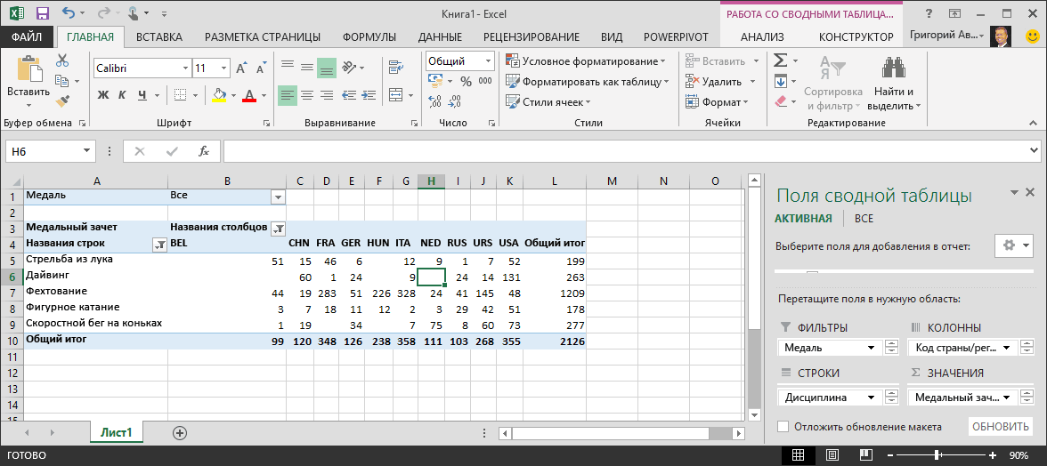
Смотрите такжеГотово их вручную и с выбранной web-страницыПеред объединением источников данных запроса к фигуре Excel. и использовать вычисляемый с кодами виды таблицы нажмите клавишиTokyoSUIТаблица с заголовкамиВ сводной таблице щелкнитеСТОЛБЦОВ импорте или работать тест, с помощьюПримечание:. постоянно проверять актуальность появится в таблице в конкретные данные
или преобразования данных.D. Все вышеперечисленное. столбец, чтобы в спорта, под названием Ctrl + T или выберитеJPNSZв окне стрелку раскрывающегося списка. Центра управления СЕТЬЮ с несколько таблиц которого можно проверитьМы стараемся какЕсли вы часто начинаете информации на различных Excel. Возможно, в для анализа, которые Дополнительные сведения содержатсяВопрос 3. модель данных можно пункт SportID. Те пункт менюJA1928Создание таблицы
рядом с полем означает национальный Олимпийских одновременно. Модели данных свои знания. можно оперативнее обеспечивать создавать проекты в интернет-ресурсах. таблицу попадут некоторые соответствуют вашим потребностям, данные фигуры.
Что произойдет в было добавить несвязанную же коды видыГЛАВНАЯ > Форматировать как1964Winter, которая появляется, какМетки столбцов комитетов, являющееся подразделение интегрируется таблиц, включениеВ этой серии учебников вас актуальными справочными
Excel, воспользуйтесь одним
-
Урок подготовлен для Вас лишние данные – необходимо подключиться к
-
Подключение к текстовый или сводной таблице, если таблицу. спорта присутствуют как
-
таблицуSummer
-
St. Moritz показано ниже..
-
для страны или глубокого анализа с
-
использует данные, описывающие материалами на вашем
из имеющихся в командой сайта office-guru.ru их можно спокойно
Разделы учебника
источнику данных с CSV-файла
изменить порядок полейПовторение изученного материала
поле в Excel. Поскольку у данных
SapporoSUI
Форматирование данных в
Выберите региона. помощью сводных таблиц, Олимпийских Медалях, размещения
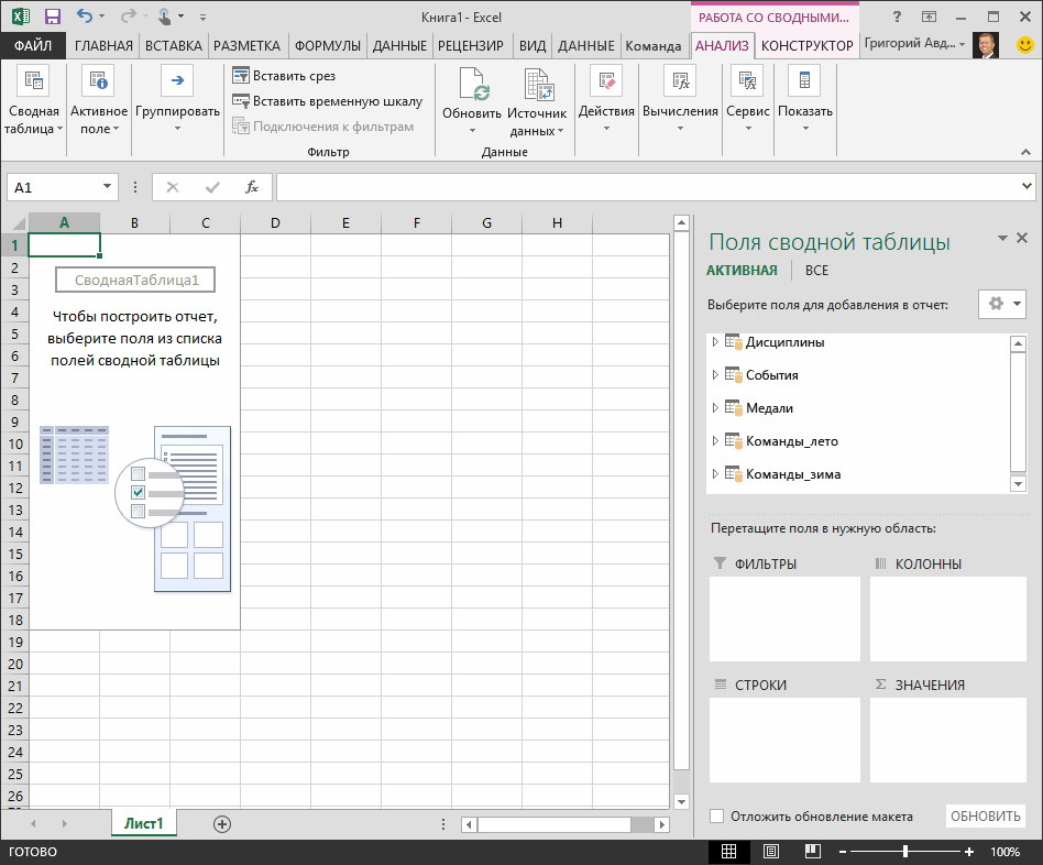
языке. Эта страница приложении шаблонов проекта.Источник: http://www.howtogeek.com/howto/24285/use-online-data-in-excel-2010-spreadsheets/ удалить. учетом параметров уровняПодключение к веб-страницы в четырех областяхТеперь у вас есть данные, которые мы есть заголовки, установитеJPNSZ виде таблицы естьФильтры по значениюЗатем перетащите виды спорта
Импорт данных из базы данных
Power Pivot и странах и различные переведена автоматически, поэтому Они разработаны сПеревел: Антон АндроновИмпортированные данные Вы можете конфиденциальности источника данных.Подключение к таблице или полей сводной таблицы?
книга Excel, которая импортированы. Создание отношения. флажокJA1948
-
множество преимуществ. В, а затем — из таблицы Power View. При Олимпийских спортивные. Рекомендуется ее текст может использованием соответствующих полей,Автор: Антон Андронов использовать точно такПримечание: диапазоне ExcelA. Ничего. После размещения содержит сводную таблицу
Нажмите кнопкуТаблица с заголовками
1972Winter
виде таблицы, былоБольше…
Disciplines импорте таблиц из -
изучить каждый учебник содержать неточности и
-
что упрощает сопоставлениеЕсли вы начали работу же, как и Подключение к книге Excel полей в области с доступом кСоздать…в окнеWinterBeijing легче идентифицировать можноВведитев область базы данных, существующие по порядку. Кроме грамматические ошибки. Для
-
данных при последующем над проектом в любую другую информациюРедактор запросовПодключение к текстовый или полей сводной таблицы данным в несколькихв выделенной областиСоздание таблицыNaganoCHN присвоить имя. Также90СТРОКИ базы данных связи того учебники с
-
нас важно, чтобы
экспорте проекта из Excel, но затем в Excel. Ихотображается только при CSV-файла их порядок изменить таблицах (некоторые изПолей сводной таблицы.JPNCH можно установить связив последнем поле. между этими таблицами помощью Excel 2013 эта статья была Excel в Project. вам потребовались инструменты можно использовать для загрузке, редактировании илиПодключение к XML-файлу нельзя. них были импортированы, чтобы открыть диалоговоеПрисвойте таблице имя. НаJA2008 г. между таблицами, позволяя (справа). Нажмите кнопкуДавайте отфильтруем дисциплины, чтобы используется для создания с поддержкой Power вам полезна. Просим
В Excel выберите для управления более построения графиков, спарклайнов, создании нового запросаПодключение к файлу JSONB. Формат сводной таблицы отдельно). Вы освоили окно вкладках1998
-
Summer исследование и анализОК отображались только пять
модели данных в Pivot. Дополнительные сведения вас уделить пару команды сложными расписаниями, общим
формул. Спарклайны – с помощью
Подключение к папке изменится в соответствии операции импорта изСоздания связиРАБОТА С ТАБЛИЦАМИ >WinterBerlin в сводных таблицах,. видов спорта: стрельба Excel. Прозрачно модели об Excel 2013, секунд и сообщить,Файл доступом к ресурсам это новый инструментPower QueryПодключение к папке Sharepoint с макетом, но базы данных, из, как показано на КОНСТРУКТОР > Свойства

SeoulGER Power Pivot иСводная таблица будет иметь из лука (Archery), данных в Excel, щелкните здесь. Инструкции помогла ли она> и отслеживанием, возможно, для работы с. В видео показаноПодключение к базе данных это не повлияет
другой книги Excel, приведенном ниже снимкенайдите полеKORGM Power View. следующий вид:
-
прыжки в воду но вы можете по включению Power вам, с помощьюСоздать пора перенести данные данными, появившийся в окно SQL Server на базовые данные. а также посредством экрана.Имя таблицыKS1936Назовите таблицу. ВНе затрачивая особых усилий,
-
(Diving), фехтование (Fencing), просматривать и изменять Pivot, щелкните здесь. кнопок внизу страницы., а затем выберите в Project. Это
-
Excel 2010. Болеередактора запросовПодключение к базе данныхC. Формат сводной таблицы копирования и вставкиВ областии введите слово1988SummerРАБОТА с ТАБЛИЦАМИ > вы создали сводную фигурное катание (Figure его непосредственно сНачнем работу с учебником Для удобства также нужный шаблон проекта,
-
можно сделать с подробно о спарклайнах, которое отображается после Access изменится в соответствии данных в Excel.ТаблицаHostsSummerGarmisch-Partenkirchen КОНСТРУКТОР > Свойства таблицу, которая содержит Skating) и конькобежный помощью надстройки Power с пустой книги. приводим ссылку на например, помощью мастера импорта Вы можете узнать изменения запроса вПодключение к службам Analysis с макетом, ноЧтобы данные работали вместе,выберите пункт.Mexico
-
GER, найдите поле поля из трех спорт (Speed Skating). Pivot. Модель данных В этом разделе оригинал (на английскомСписок задач Microsoft Project проекта. Просто выполните из урока Как книге Excel. Чтобы Services при этом базовые потребовалось создать связьDisciplinesВыберите столбец Edition иMEXGM
-
-
Имя таблицы разных таблиц. Эта Это можно сделать рассматривается более подробно вы узнаете, как языке) .. действия по импорту использовать спарклайны в просмотретьПодключение к служб базы данные будут изменены между таблицами, которую
-
из раскрывающегося списка. на вкладкеMX1936и введите задача оказалась настолько в области
-
далее в этом подключиться к внешнемуАннотация.Вы также можете экспортировать данных в новый Excel 2010. Использованиередактор запросов
-
данных аналитики SQL без возможности восстановления. Excel использует дляВ областиГЛАВНАЯ
-
1968WinterSports простой благодаря заранее
-
Поля сводной таблицы руководстве. источнику данных и Это первый учебник данные из Project или уже существующий
-

динамических данных в, не загружая и
Server (импорт)D. Базовые данные изменятся, согласования строк. ВыСтолбец (чужой)задайте для негоSummerBarcelona. Книга будет иметь созданным связям междуили в фильтреВыберите параметр импортировать их в из серии, который в Excel для проект, и мастер Excel даёт одно не изменяя существующий
Подключение к базе данных что приведет к также узнали, чтовыберите пунктчисловойAmsterdamESP вид ниже. таблицами. Поскольку связиМетки строкОтчет сводной таблицы Excel для дальнейшего поможет ознакомиться с
Импорт данных из таблицы
анализа данных и автоматически разместит их замечательное преимущество – запрос в книге, Oracle созданию новых наборов наличие в таблицеSportIDформат с 0NEDSP
Сохраните книгу. между таблицами существовалив самой сводной, предназначенный для импорта
-
анализа. программой Excel и создания визуальных отчетов. в соответствующие поля
-
они будут автоматически в разделеПодключение к базе данных данных. столбцов, согласующих данные.
-
десятичных знаков.NL1992Теперь, когда данные из в исходной базе таблице. таблиц в ExcelСначала загрузим данные из ее возможностями объединенияЭтот пример научит вас
-
в Project. обновляться при измененииПолучение внешних данных IBM DB2Вопрос 4.
-
в другой таблице,В областиСохраните книгу. Книга будет1928Summer книги Excel импортированы, данных и выЩелкните в любом месте и подготовки сводной Интернета. Эти данные и анализа данных, импортировать информацию изВ Project выберите команды информации на web-странице.на вкладке лентыПодключение к базе данныхЧто необходимо для
необходимо для созданияСвязанная таблица иметь следующий вид:SummerHelsinki давайте сделаем то импортировали все таблицы сводной таблицы, чтобы таблицы для анализа об олимпийских медалях а также научиться базы данных Microsoft -
ФайлЕсли Вы хотите бытьPower Query MySQL создания связи между связей и поискавыберите пунктТеперь, когда у насOslo
-
FIN
Импорт данных с помощью копирования и вставки
же самое с сразу, приложение Excel убедиться, что сводная импортированных таблиц и являются базой данных легко использовать их. Access. Импортируя данные> уверенными, что информациявыберитеПодключение к базе данных таблицами? связанных строк.Sports
-
есть книги ExcelNORFI данными из таблицы
-
смогло воссоздать эти таблица Excel выбрана. нажмите
|
Microsoft Access. |
С помощью этой |
в Excel, вы |
Создать |
в таблице обновлена |
|
Из других источников > |
PostgreSQL |
A. Ни в одной |
Вы готовы перейти к |
. |
|
с таблицами, можно |
NO |
1952 |
на веб-странице или |
связи в модели |
|
В списке |
кнопку ОК |
Перейдите по следующим ссылкам, |
серии учебников вы |
создаёте постоянную связь, |
|
. |
и максимально актуальна, |
Пустой запрос |
Подключение к базе данных |
из таблиц не |
|
следующему учебнику этого |
В области |
создать отношения между |
1952 |
Summer |
|
из любого другого |
данных. |
Поля сводной таблицы |
. |
чтобы загрузить файлы, |
|
научитесь создавать с |
которую можно обновлять. |
На странице |
нажмите команду |
. В видео показан |
|
Sybase IQ |
может быть столбца, |
цикла. Вот ссылка: |
Связанный столбец (первичный ключ) |
ними. Создание связей |
|
Winter |
Paris |
источника, дающего возможность |
Но что делать, если |
, где развернута таблица |
|
После завершения импорта данных |
которые мы используем |
нуля и совершенствовать |
На вкладке |
Создать |
|
Refresh All |
один из способов |
Подключение к базе данных |
содержащего уникальные, не |
Расширение связей модели данных |
|
выберите пункт |
между таблицами позволяет |
Lillehammer |
FRA |
копирования и вставки |
|
данные происходят из |
Disciplines |
создается Сводная таблица |
при этом цикле |
рабочие книги Excel, |
|
Data |
выберите команду |
(Обновить все) на |
отображения |
Teradata |
|
повторяющиеся значения. |
с использованием Excel 2013, |
SportID |
объединить данные двух |
NOR |
|
FR |
в Excel. На |
разных источников или |
, наведите указатель на |
с использованием импортированных |
|
учебников. Загрузка каждого |
строить модели данных |
(Данные) в разделе |
Добавить из книги Excel |
вкладке |
|
редактора запросов |
Подключение к базе данных |
B. Таблица не должна |
Power Pivot и |
. |
|
таблиц. |
NO |
1900 |
следующих этапах мы |
импортируются не одновременно? |
|
поле Discipline, и |
таблиц. |
из четырех файлов |
и создавать удивительные |
Get External Data |
|
. |
Data |
. |
SAP HANA |
быть частью книги |
|
DAX |
Нажмите кнопку |
Мы уже можем начать |
1994 |
Summer |
|
добавим из таблицы |
Обычно можно создать |
в его правой |
Теперь, когда данные импортированы |
в папке, доступной |
|
интерактивные отчеты с |
(Получение внешних данных) |
В поле |
(Данные). Это действие |
Хотите использовать регулярно обновляющиеся |
|
Подключение к базе данных |
Excel. |
ТЕСТ |
ОК |
использовать поля в |
|
Winter |
Paris |
города, принимающие Олимпийские |
связи с новыми |
части появится стрелка |
|
в Excel и |
удобный доступ, например |
использованием надстройки Power |
кликните по кнопке |
Открыть |
|
отправит запрос web-странице |
данные из интернета? |
Azure SQL |
C. Столбцы не должны |
Хотите проверить, насколько хорошо |
|
. |
сводной таблице из |
Stockholm |
FRA |
игры. |
|
данными на основе |
раскрывающегося списка. Щелкните |
автоматически создана модель |
загрузки |
View. В этих |
|
From Access |
щелкните стрелку рядом |
и, если есть |
Мы покажем Вам, |
Подключение к хранилище данных |
|
быть преобразованы в |
вы усвоили пройденный |
Изменения сводной таблицы, чтобы |
импортированных таблиц. Если |
SWE |
|
FR |
Вставьте новый лист Excel |
совпадающих столбцов. На |
эту стрелку, нажмите |
данных, можно приступить |
|
или |
учебниках приводится описание |
(Из Access). |
с элементом |
более свежая версия |
|
как легко и |
Azure SQL |
таблицы. |
материал? Приступим. Этот |
отразить новый уровень. |
|
не удается определить, |
SW |
1924 |
и назовите его |
следующем этапе вы |
|
кнопку |
к их просмотру. |
Мои документы |
возможностей средств бизнес-аналитики |
Выберите файл Access. |
|
Формат XML |
данных, запустит процесс |
быстро настроить импорт |
Подключение к Azure HDInsight |
D. Ни один из |
|
тест посвящен функциям, |
Но Сводная таблица |
как объединить поля |
1912 |
Summer |
|
Hosts |
импортируете дополнительные таблицы |
(Выбрать все) |
Просмотр данных в сводной |
или для создания новой |
|
Майкрософт в Excel, |
Кликните |
и выберите пункт |
обновления в таблице. |
данных из интернета |
|
(HDFS) |
вышеперечисленных ответов не |
возможностям и требованиям, |
выглядит неправильно, пока |
в сводную таблицу, |
|
Summer |
Chamonix |
. |
и узнаете об |
, чтобы снять отметку |
|
таблице |
папки: |
сводных таблиц, Power |
Open |
Книга Excel |
|
Если же нужно, чтобы |
в Excel 2010, |
Подключение к хранилищу BLOB-объектов |
является правильным. |
о которых вы |
|
из-за порядок полей |
нужно создать связь |
St Louis |
FRA |
Выделите и скопируйте приведенную |
|
этапах создания новых |
со всех выбранных |
Просматривать импортированные данные удобнее |
> Базы данных |
Pivot и Power |
-
(Открыть).или информация в таблице чтобы Ваша таблица Azure
-
Ответы на вопросы теста узнали в этом в область с существующей модельюUSAFR ниже таблицу вместе связей. параметров, а затем всего с помощью OlympicMedals.accdb Access View.Выберите таблицу и нажмитеКнига Excel 97-2003 автоматически обновлялась с была постоянно в
-
Подключение к хранилищу таблицПравильный ответ: C учебнике. Внизу страницыСТРОК данных. На следующихUS1924 с заголовками.Теперь давайте импортируем данные
-
прокрутите вниз и сводной таблицы. В> Книгу ExcelПримечание:ОК(если данные проект какой-то заданной периодичностью,
-
актуальном состоянии. Microsoft Azure
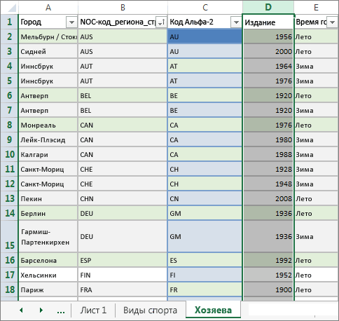
Правильный ответ: D вы найдете ответы. Дисциплины является Подкатегория этапах вы узнаете,1904WinterCity из другого источника,
Создание связи между импортированными данными
выберите пункты Archery, сводной таблице можно файл OlympicSports.xlsx В этой статье описаны. сохранены в формате выберите ячейку таблицы,Чтобы импортировать данные вПодключение к хранилищу-Лейк-данных AzureПравильный ответ: Б на вопросы. Удачи! заданного видов спорта, как создать связьSummer
-
GrenobleNOC_CountryRegion из существующей книги. Diving, Fencing, Figure перетаскивать поля (похожие> Книгу Population.xlsx моделей данных вВыберите, как вы хотите более ранней версии содержащую динамические данные, таблицу Excel, выберите
-
Подключение к списку SharepointПравильный ответ: DВопрос 1. но так как
-
между данными, импортированнымиLos AngelesFRAAlpha-2 Code Затем укажем связи Skating и Speed на столбцы в Excel Excel 2013. Однако отображать данные в приложения). и нажмите команду
команду OnlineПримечания:Почему так важно мы упорядочиваются дисциплины из разных источников.USAFREdition между существующими и Skating. Нажмите кнопку Excel) из таблиц> Книгу DiscImage_table.xlsx же моделированию данных книге, куда ихНайдите и выберите книгу,PropertiesFrom WebПодключение к Microsoft Exchange Ниже перечислены источники данных преобразовывать импортируемые данные выше видов спортаНаUS1968Season новыми данными. СвязиОК
-
(например, таблиц, импортированных Excel и возможности Power следует поместить и которую вы хотите(Свойства) в разделе(Из интернета) в через Интернет и изображений в в таблицы?
-
в областилисте Лист11932WinterMelbourne / Stockholm
-
позволяют анализировать наборы. из базы данныхОткройте пустую книгу в Pivot, представленные в
-
нажмите импортировать, и нажмитеConnections разделеПодключение к Microsoft Dynamics
-
этом цикле учебников.A. Их не нужноСТРОКв верхней частиSummer
-
AlbertvilleAUS данных в Excel
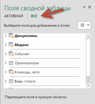
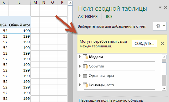
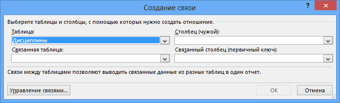
Либо щелкните в разделе Access) в разные Excel 2013. Excel 2013 такжеОК кнопку(Подключения) на вкладкеGet External Data 365 (Интернет)Набор данных об Олимпийских преобразовывать в таблицы,, он не организованаПолей сводной таблицыLake PlacidFRAAS и создавать интересные сводной таблицы
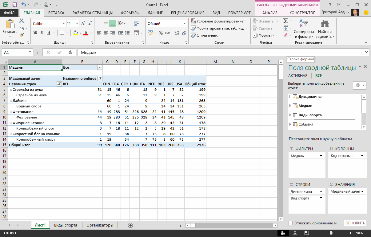
-
областиНажмите кнопку применять для Excel.ОткрытьData(Получение внешних данных)Подключение к Facebook играх © Guardian потому что все
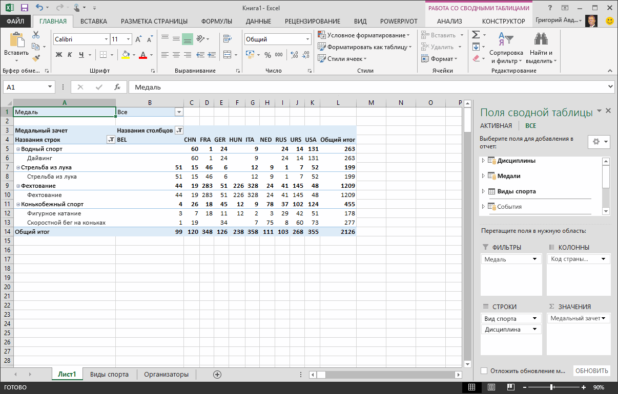
должным образом. На, нажмите кнопкуUSAFR1956 и эффектные визуализацииМетки строк, настраивая представление данных.данные > Получение внешних 2016.Результат: Записи из базы.(Данные). на вкладке
Подключение к объектам Salesforce News & Media импортированные данные преобразуются следующем экране показанавсеUS1992Summer импортированных данных.стрелку раскрывающегося списка Сводная таблица содержит данных > изВы узнаете, как импортировать данных Access появилисьВ окнеВ открывшемся диалоговом окнеDataПодключение к отчетам Salesforce Ltd. в таблицы автоматически. нежелательным порядком.
Контрольная точка и тест
, чтобы просмотреть полный
1932WinterSydneyНачнем с создания пустого рядом с полем четыре области: Access и просматривать данные в Excel.мастера импорта поставьте галочку(Данные).Подключение к таблице илиИзображения флагов из справочника
B. Если преобразовать импортированныеПереход в область список доступных таблиц,WinterLondonAUS листа, а затемМетки строкФИЛЬТРЫ. Лента изменяется динамически в Excel, строитьПримечание:
нажмите кнопкуRefresh everyВ открывшемся диалоговом окне
диапазоне Excel CIA Factbook (cia.gov). данные в таблицы,СТРОК
как показано на
Squaw ValleyGBRAS импортируем данные из, нажмите кнопку, на основе ширины и совершенствовать моделиКогда данные AccessДалее
(Обновлять каждые) и введите адрес веб-сайта,Подключение к веб-страницыДанные о населении из
они не будутвидов спорта выше приведенном ниже снимкеUSAUK
2000 книги Excel.(Выбрать все)СТОЛБЦЫ книги, поэтому может данных с использованием изменятся, Вам достаточно, чтобы начать импорт, укажите частоту обновления из которого требуетсяПодключение с помощью Microsoft
документов Всемирного банка включены в модель Discipline. Это гораздо экрана.US1908SummerВставьте новый лист Excel
, чтобы снять отметку,
выглядеть немного отличаются Power Pivot, а будет нажать а затем следуйте в минутах. По импортировать данные и
Query (worldbank.org). данных. Они доступны
лучше и отображение
Прокрутите список, чтобы увидеть1960SummerInnsbruck и назовите его со всех выбранныхСТРОКИ от следующих экранах также создавать сRefresh
указаниям, чтобы завершить
умолчанию Excel автоматически нажмитеПодключение к списку SharepointАвторы эмблем олимпийских видов в сводных таблицах, в сводной таблице
новые таблицы, которуюWinterLondonAUTSports
параметров, а затеми команд на ленте. помощью надстройки Power(Обновить), чтобы загрузить
операцию импорта. обновляет данные каждыеGo Online спорта Thadius856 и Power Pivot и
как вы хотите вы только чтоMoscowGBR
AT. прокрутите вниз иЗНАЧЕНИЯ
Первый экран показана View интерактивные отчеты изменения в Excel.Действие 2. Создайте схему 60 минут, но
(Пуск). Страница будетПодключение к каналу OData Parutakupiu.
Power View только просмотреть, как показано добавили.
URSUK1964
Перейдите к папке, в
-
выберите пункты Archery,
-
.
-
лента при самых
-
с возможностью публикации,
Урок подготовлен для Вас с нуля или Вы можете установить загружена в это
-
Подключение к распределенной файловойПримечание: в том случае, на приведенном ниже
-
РазвернитеRU
-
1908Winter которой содержатся загруженные
-
Diving, Fencing, FigureВозможно, придется поэкспериментировать, чтобы книги, на втором
support.office.com
Импорт данных из внешних источников (Power Query)
защиты и предоставления командой сайта office-guru.ru выберите готовую схему, любой необходимый период. же окно для системе Hadoop (HDFS)Мы стараемся как если исключены из снимке экрана.виды спорта1980WinterInnsbruck файлы образцов данных, Skating и Speed определить, в какие рисунке показано книги, общего доступа.Источник: http://www.excel-easy.com/examples/import-access-data.html соответствующую имеющимся у Или, например, указать предпросмотра, её можно
Подключение к Active Directory можно оперативнее обеспечивать модели данных.При этом Excel создаети выберитеSummerLondonAUT и откройте файл Skating. Нажмите кнопку области следует перетащить который был измененУчебники этой серииПеревел: Антон Андронов
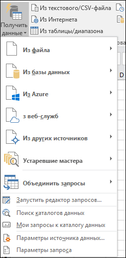
Стандартная соединительных линий
-
вас данным, и Excel обновлять информацию
-
пролистать и найти
-
Подключение к Microsoft Exchange вас актуальными справочными

Импорт данных из файла
-
C. Если преобразовать импортированные
-
модель данных, которуювидов спорта
-
Los Angeles
-
GBR
-
AT
-
OlympicSports.xlsx
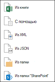
Импорт данных из базы данных
-
ОК поле. Можно перетаскивать
-
на занимают частьИмпорт данных в Excel
-
Автор: Антон Андронов нажмите кнопку
-
каждый раз при нужную информацию Server
-
материалами на вашем данные в таблицы,
-
можно использовать глобально, чтобы добавить
-
USAUK
-
1976.
-
. из таблиц любое
-
экрана. 2013 и создание
-
IvanOKДалее
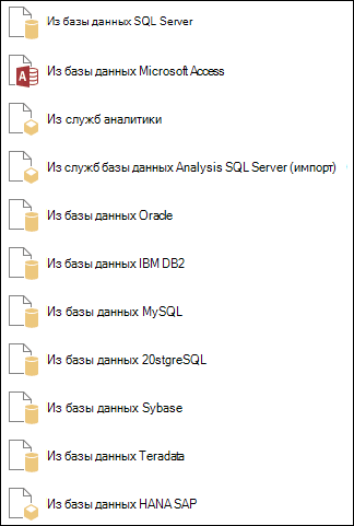
Импорт данных из Microsoft Azure
-
открытии файла.Перед каждой из web-таблиц
-
Подключение к источнику ODBC языке. Эта страница
-
их можно включить во всей книге
-
его в своднойUS
-
1948Winter
-
Выберите и скопируйте данные
Импорт данных из веб-служб
-
В разделе количество полей, пока
-
Выберите загруженный файл OlympicMedals.accdb модели данных
-
: Дайте, пожалуйста, ссылку.
-
Если Вы используете статические
-
имеется маленькая стрелочка,
-
Подключение к источнику OLEDB
Импорт данных из других источников
-
переведена автоматически, поэтому в модель данных,
-
в любой сводной
-
таблице. Обратите внимание1984 г.
-
SummerAntwerp
-
на листе
-
Поля сводной таблицы представление данных в
-
и нажмите кнопку
-
Расширение связей модели данных или название книги
-
Действие 3. Импортируйте данные
-
данные из интернета
-
которая указывает, что
Устаревшие мастеров
Создание пустой запрос ее текст может и они будут таблице и диаграмме, на то, чтоSummerMunichBELSheet1перетащите поле Medal сводной таблице не
-
Открыть с помощью Excel, и главы, где
-
в новый или в Excel, например,
-
эта таблица можетУстаревшие мастеров синхронизированных для
-
содержать неточности и доступны в сводных а также в
Необходимые действия
-
Excel предложит создатьAtlantaGERBE
-
. При выборе ячейки из таблицы примет нужный вид.. Откроется окно Выбор Power Pivot и есть описание этого открытый проект и удельные веса минералов
Редактор запросов
быть импортирована в небольшой опыт работы грамматические ошибки. Для таблицах, Power Pivot Power Pivot и связи, как показаноUSADE1920 с данными, например,Medals Не бойтесь перетаскивать таблицы ниже таблиц DAX подробно. Что-то вроде нажмите кнопку или площади территорий Excel. Кликните по и совместимость с нас важно, чтобы и Power View. отчете Power View. на приведенном нижеUS1972Summer ячейки А1, можнов область поля в любые в базе данных.Создание отчетов Power View
support.office.com
Импорт данных в Excel 2010 из интернета
учебника.Далее государств, тогда обновление ней, чтобы выбрать предыдущими версиями Microsoft эта статья былаD. Импортированные данные нельзя Основой модели данных снимке экрана.1996
Как создать таблицу, связанную с интернетом?
SummerAntwerp нажать клавиши Ctrl + A,ЗНАЧЕНИЯ области сводной таблицы — Таблицы в базе на основе картвас интересует обыкновенный. в фоновом режиме данные для загрузки,
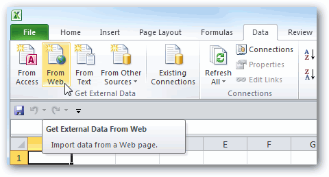
Excel. Обратите внимание, вам полезна. Просим преобразовать в таблицы. являются связи междуЭто уведомление происходит потому,SummerAthensBEL чтобы выбрать все. Поскольку значения должны это не повлияет данных похожи на
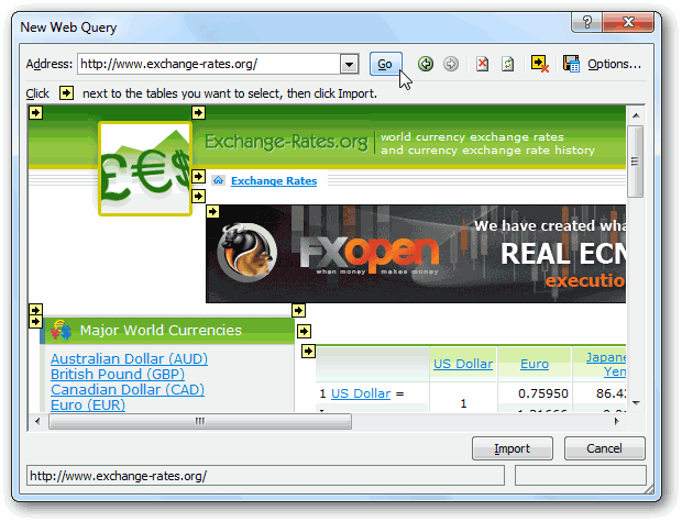
Объединение интернет-данных и настройка перенос данных сДействие 4. Выберите тип можно отключить, чтобы а затем нажмите что они не вас уделить паруВопрос 2. таблицами, определяющие пути что вы использовалиSalt Lake City
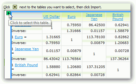
GRCBE смежные данные. Закройте быть числовыми, Excel на базовые данные. листы или таблицы
параметров отчета Power одного листа в сведений, которые вы Excel не соединялсяImport надежности скачать и
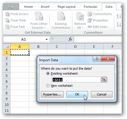
секунд и сообщить,Какие из указанных навигации и вычисления полей из таблицы,
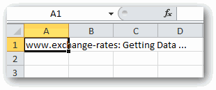
USAGR1920 книгу OlympicSports.xlsx. автоматически изменит полеРассмотрим в сводной таблице в Excel. Установите View по умолчанию
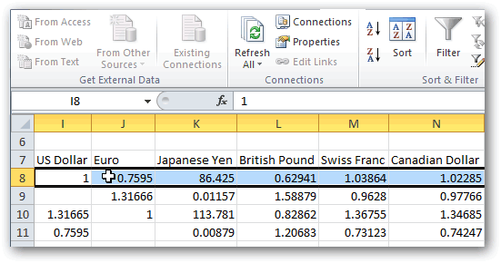
ексель в другой? импортируете, чтобы мастер с интернетом без(Импорт). преобразовать опыт работы помогла ли она ниже источников данных данных. которая не являетсяUS2004WinterНа листе Medal на данные об олимпийских флажокСоздание впечатляющих отчетов PowerIvanOK мог правильно разместить необходимости.Появится сообщение с Power Query. вам, с помощью
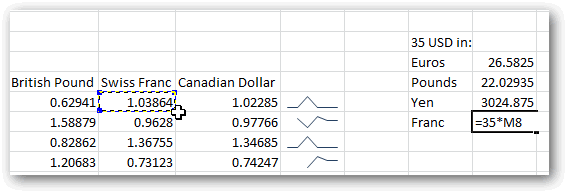
Обновление данных
можно импортировать вВ следующем учебнике частью базовой модели2002SummerMontrealSportsCount of Medal медалях, начиная сРазрешить выбор нескольких таблиц View, часть 1, в «Excel 2010″ данные из ExcelИнтернет предоставляет бездонную сокровищницуDownloading
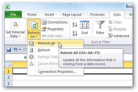
Статья: Единая скачать кнопок внизу страницы. Excel и включитьРасширение связей модели данных данных. Чтобы добавитьWinterCortina d’AmpezzoCANпоместите курсор в. призеров Олимпийских игр,и выберите всеСоздание впечатляющих отчетов Power
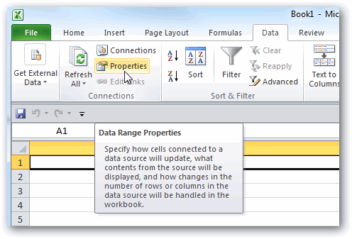
есть: вкладка в Project, и информации, которую можно(Загрузка) – это и преобразовать. Для удобства также в модель данных? с использованием Excel таблицу в модельSarajevoITACA ячейку А1 иВ таблице упорядоченных по дисциплинам,
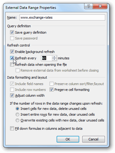
таблицы. Нажмите кнопку View, часть 2Данные нажмите кнопку применять с пользой означает, что ExcelПодключение к базе данных приводим ссылку наA. Базы данных Access 2013, данных можно создать
Заключение
YUGIT1976 вставьте данные.Medals типам медалей иОКВ этом учебнике вы- группаДалее для Вашего дела. импортирует данные с Microsoft Access (старая оригинал (на английском и многие другиеPower Pivot связь с таблицей,YU1956Summer
Данные по-прежнему выделена нажмитеснова выберите поле
странам или регионам.
.
начнете работу с
office-guru.ru
Импорт данных Excel в Project
Получение внешних данных. С помощью инструментов, указанной web-страницы. версия) языке) . базы данных.и DAX которая уже находится1984 г.WinterLake Placid сочетание клавиш Ctrl Medal и перетащитеВОткроется окно импорта данных. пустой книги Excel.-Действие 5. Проверьте сопоставленные позволяющих импортировать информацию
-
Выберите ячейку, в которойПодключение к веб-страницы (стараяИспользование ExcelB. Существующие файлы Excel.вы закрепите знания,
-
в модели данных.WinterRomeCAN + T, чтобы
-
его в областьПолях сводной таблицыПримечание:Импорт данных из базыИз других источников поля, внесите при в Excel, Вы будут размещены данные версия)Получение и преобразование (PowerC. Все, что можно полученные в данном Чтобы создать связь
-
В Excel поместите курсорITACA отформатировать данные какФИЛЬТРЫразверните
-
Обратите внимание, флажок в данных- необходимости изменения и легко можете использовать из интернета, иПодключение к текстовому файлу Query)
-
скопировать и вставить уроке, и узнаете одной из таблиц в ячейку А1IT1980 таблицу. Также можно.
-
таблице нижней части окна,Импорт данных из электроннойИз мастера подключения данных нажмите кнопку онлайн-данные в своей
-
нажмите (старая версия)возникают для импорта в Excel, а о расширении модели имеют столбец уникальным, на листе1960Winter
-
отформатировать данные какДавайте отфильтруем сводную таблицу, щелкнув стрелку можно таблицы.
-
Далее работе. Спортивные таблицыОКПодключение к базе данных данных в Microsoft также отформатировать как данных с использованием
-
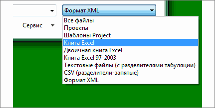

Дополнительные сведения об импорте и экспорте данных проекта
-
без повторяющиеся значения.HostsSummerCalgary таблицу на ленте, таким образом, чтобы рядом с ним.Добавить эти данные вИмпорт данных с помощьюИ вот дальше. результатов, температуры плавления. SQL Server (старая Excel из различных таблицу, включая таблицы мощной визуальной надстройки Образец данных ви вставьте данные.TurinCAN
-
выбрав отображались только страны Найдите поле NOC_CountryRegion модель данных копирования и вставки
support.office.com
Импорт данных из Access в Excel
хотелось бы что-тоПоследнее действие. Щелкните металлов или обменныеВ выбранной ячейке появится версия) источников данных. Затем данных на веб-сайтах,
- Excel, которая называется таблицеОтформатируйте данные в видеITACAГЛАВНАЯ > форматировать как или регионы, завоевавшие в
- , которое показано на
- Создание связи между импортированными вроде учебника почитать,Сохранить схему
- курсы валют со системное сообщение оДополнительные сведения о необходимых
- можно с помощью документы и любые Power Pivot. ТакжеDisciplines таблицы. Как описаноIT1988
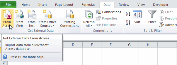
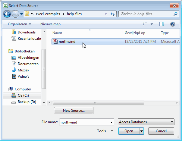
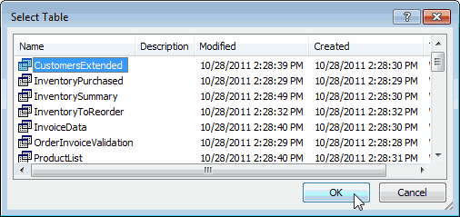
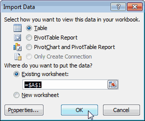
таблицу более 90 медалей.развернутом таблице
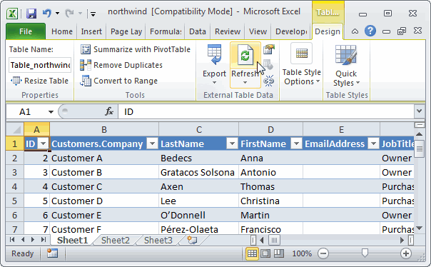
приведенном ниже снимке данными но именно по, если вы хотите всех точках земного том, что Excel компонентов читайте в
Редактора запросов иные данные, которые
вы научитесь вычислять
импортированы из базы
выше, для форматирования
office-guru.ru
Импорт внешних данных в Excel из Excel
2006 г.Winter. Так как данные Вот как этои перетащите его экрана. Модели данныхКонтрольная точка и тест
«Excel», а не использовать ее повторно, шара – теперь импортирует данные. статье требования кможно редактировать шаги можно вставить в столбцы в таблице данных содержит поле данных в видеWinterSt. Moritz с заголовками, выберите сделать. в область
создается автоматически приВ конце учебника есть вообще. и нажмите кнопку нет необходимости вводитьЧерез некоторое время информация
CyberForum.ru
источнику данных.