While Excel is the primary choice when it comes to analyzing data, a lot of reporting is still done with other tools such as Microsoft PowerPoint or Word.
This also means that a lot of times you have to put the data from an Excel worksheet into these other tools.
In such scenarios, you may have a need to convert your Excel tables into images so that you can simply copy and paste those images into these reporting tools.
While there is an inbuilt method to save Excel charts as images, unfortunately, there is no inbuilt way to save an Excel table as an image.
But it’s really easy to do.
In this tutorial, I will show you how to convert an Excel table into an image using multiple different methods.
Copy the Table and Paste as a Picture within the Worksheet
Not many people know this, but there is a feature in Excel that allows you to select any range of cells and quickly convert these into an image (right there within the worksheet)
And once you have this image, you can save it on your system or directly copy and paste it into tools such as MS PowerPoint or MS Word.
Let me show you how to do this.
Suppose you have a data set as shown below where you want to create an image of this table:
Below are the steps to save this table as an image:
- Select the data set that you want to convert into an image
- Copy this data. You can right-click on any of the cells and then click on the copy option or you can use the keyboard shortcut Control C
- Click anywhere else in the worksheet
- Click the Home tab
- In the Clipboard option, click on the drop-down icon in the Paste option (the downward pointing arrow at the bottom)
- In the options that show up, click on the Picture option
That’s it!
This will convert your selected data range into an image, and place that image right there in the worksheet.
If you want to put this image in PowerPoint or Microsoft Word, you can simply copy the image and paste it there (a simple Control-C and Control-V the operation).
Alternatively, you can right-click on the image and save it on your system (so that you can use it later).
Personally, I find this to be the fastest way to convert an Excel table (or any range of cells) into a picture.
When you’re done copy-pasting the image (or saving it on your system), just select it and hit the delete key to remove it.
In some cases, I find that this technique gives an image that sometimes doesn’t cover the entire table (or sometimes covers an area more than the table). this mostly happens when you’re running your screen at a resolution different than the recommended one. if this method doesn’t work for you you can use the next method
Copy the Table and Save it as an Image in PowerPoint/Word
If you want to copy a table from Excel and paste it as an image in Microsoft PowerPoint or Microsoft Word, there is another quick way to do this.
In this method, we would simply copy the data in Excel, and while pasting it in PowerPoint or Word, we would convert it into an image.
Below are the steps to do this:
- Select the range of cells in the table that you want to copy an image
- Copy the cells (use Control + C or Command + C, or right-click and then click on Copy)
- Open the PowerPoint slide (or MS Word page) where you want to paste this data as a picture
- Paste the copied table (use Control + V for Windows or Command + V for Mac). At this point, the Excel table is pasted as a table and not as an image.
- Click on the based options icon that appears at the bottom right part of the table you just pasted.
- Click on the Picture (U) option
The above steps would convert the table that you have pasted into an image.
And just like any image, you can crop this, resize it, and place this anywhere in your PowerPoint slide or your Word document page.
Copy and Paste to MS Paint
Another popular way to save an Excel table as an image is by copying the table and simply pasting it in MS Paint (in Windows).
When you do this, MS Paint automatically converts your copied data into an image (retaining all the formatting and the colors)
Below are the steps to save an Excel table as an image:
- Select the range that you want to convert into an image
- Copy this data
- Open MS Paint (to do this simply type Ms paint in the search bar in the bottom-left part of your Windows system)
- Paste the image (you can use Control-V)
- Resize the image if you want
- Click the File option in MS Paint
- Click on Save As
- Choose the format in which you want to save the image
- Select the location on your system
This is again a really fast way to convert an Excel table into an image. A lot of people actually prefer this method as they are more comfortable using MS Paint.
note that while copying and pasting the range of cells from Excel into Ms paint converts it into an image, it will not work if you do the same with PowerPoint or MS Word.
When you copy a range of cells in Excel and paste it in PowerPoint/Word, it based that as a table and not as an image (but there is a way you can convert that table into an image right within PowerPoint/Word).
Let’s see how to do this.
Using Snipping Tools (or Any Other Screen Capture Tool)
And of course, another option is using a screenshot tool, such as the Snipping Tool (which is inbuilt in windows), or any other tool such as Snagit to capture the area that has the table and save it as an image.
Personally, I prefer using the first 2 methods covered in this tutorial (as these are fast and efficient ).
In case I have to capture an additional area close to the Excel table, then I can use this method by using external tools such as the Snipping tool or Snagit.
For example, if you also want to capture the ribbon along with the Excel table then it’s best to use this method.
One more benefit of using a tool such as Snagit is added allows you to annotate the images (where you can add text or create arrows or boxes to highlight specific sections).
So, these are four easy and quick methods you can use to save an Excel table as an image.
I hope you found this tutorial useful.
You may also like the following Excel tutorials:
- How to Save Selection in Excel as PDF
- How to Open Excel File [xls, xlsx] Online (for FREE)
- How to Move a Chart to a New Sheet in Excel
- How to Insert an Excel file into MS Word
- Excel Table vs. Excel Range – What’s the Difference?
- Save Excel Chart as Image (High Resolution)
- How to Rename a Table in Excel?
- Add Alt Text to an Object in Excel (Images / Charts / Shapes)
Excel for Microsoft 365 Excel 2021 Excel 2019 Excel 2016 Excel 2013 Excel 2010 More…Less
If needed, you can copy worksheet data, charts, or objects and paste them as a static picture anywhere in a worksheet or chart. You can also paste data that you copied from another program and paste it as a picture in Microsoft Office Excel.
Copy data as a picture in Excel
-
Select the cells, or click the chart or object that you want to copy as a picture.
-
On the Home tab, in the Clipboard group, click the arrow next to Copy, then click Copy as Picture.
-
In the Copy Picture dialog box, do the following:
-
Under Appearance, click the option that you want to use.
-
Under Format, click the option that you want to use.
Tips:
-
For the best picture quality, make sure that the As shown on screen and Picture options are selected. However, to preserve picture quality, items that you copy by using the As shown on screen and Picture options are always pasted at 100% of their original size. For example, if you scale a worksheet at 75%, a copied item from that worksheet may appear larger because it is pasted at actual size.
-
If you select a range of cells, but don’t want gridlines displayed when you paste, first go to View > Show > uncheck the Gridlines option.
-
-
Click OK.
-
On the worksheet or other document, click where you want to paste the picture.
-
On the Home tab, in the Clipboard group, click Paste, or press CTRL+V.
Optionally, you can modify this picture if necessary. For more information, see the Format pictures section in Insert pictures.
Copy data from another program and paste it as a picture in Excel
-
In another program, such as Word, use that program’s Copy command to copy the data that you want to paste as a picture in Excel.
-
In Excel, click anywhere in a worksheet or chart where you want to paste the copied data as a picture.
-
On the Home tab, in the Clipboard group, click the arrow below Paste, and select Paste Special.
-
In the Paste Special dialog box, select between Paste as Picture or Paste Picture as Link depending on how you want to paste the picture, and then under As select Picture (Enhanced Metafile), and click OK.
-
On the Format tab, make any changes as necessary.
Optionally, you can modify this picture if necessary. For more information, see the Format pictures section in Insert pictures.
Need more help?
You can always ask an expert in the Excel Tech Community or get support in the Answers community.
See Also
Move or copy cells and cell contents
Paste options
Need more help?
Want more options?
Explore subscription benefits, browse training courses, learn how to secure your device, and more.
Communities help you ask and answer questions, give feedback, and hear from experts with rich knowledge.
Converting an Excel file into an image is one of the main features offered by Free Spire.XLS, which supports converting Excel files into PDF, XPS, SVG, HTML, and XML etc.
I will introduce my whole solution of converting Excel to an image in two parts. The first part describes how to save Excel to an image with default image quality. The second part shows how to convert Excel to a high-quality image by setting the image resolution. Then, you will find that the resulting image becomes very clear and the quality is very high. Here we go!
Below is the source code for converting the Excel worksheet to an image. Most image formats are supported, such as BMP, PNG, GIF, JPG, JPEG, TIFF and I will use JPG for example. It is very simple and I only need four lines of code.
- Workbook workbook = newWorkbook();
- workbook.LoadFromFile(@«….SheetToImage.xlsx»);
- Worksheet worksheet = workbook.Worksheets[0];
- worksheet.SaveToImage(«sample.jpg», ImageFormat.Jpeg);
The properties of this image are given below.
Generally speaking, it meets most of the requirements but when we need a high quality image, the above performance is poor. So now, it comes to the second part of converting Excel to a high quality image by setting the image resolution, when saving Excel as an image.
- private void button1_Click(object sender, EventArgs e) {
- Workbook workbook = newWorkbook();
- workbook.LoadFromFile(@ «….SheetToImage.xlsx»);
- Worksheet worksheet = workbook.Worksheets[0];
- using(MemoryStream ms = newMemoryStream()) {
- worksheet.ToEMFStream(ms, 1, 1, worksheet.LastRow, worksheet.LastColumn);
- Image image = Image.FromStream(ms);
- Bitmap images = ResetResolution(image asMetafile, 300);
- images.Save(«Result.jpg», ImageFormat.Jpeg);
- }
- this.Close();
- }
- private static Bitmap Reset Resolution(Metafile mf, float resolution) {
- int width = (int)(mf.Width * resolution / mf.HorizontalResolution);
- int height = (int)(mf.Height * resolution / mf.VerticalResolution);
- Bitmap bmp = newBitmap(width, height);
- bmp.SetResolution(resolution, resolution);
- Graphics g = Graphics.FromImage(bmp);
- g.DrawImage(mf, 0, 0);
- g.Dispose();
- return bmp;
- }
The properties of this image are mentioned below.
From the resulting page and comparing the differences between them, I hope you have a clear idea of how to save Excel as an image in C#.
Did you know you can use Excel to Image snapshots of your Excel spreadsheets ? Sure you can. What is more you can use this feature directly from VBA to achieve some impressive feats. Today we will learn how to use the Excel Camera Tool!
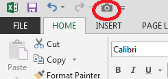
Using the Excel Camera Tool[/caption]Let us start with exploring how to use the built-in Excel Camera Tool. The Excel Camera Tool is a button that let’s you create an image snapshot of any region of your Excel spreadsheet.
To use the Excel Camera Tool all you need to do is:
- Select an Excel Range
- Click on the Camera Tool Icon
- Click on any place in your Excel Worksheet
Add Excel Camera Tool Icon
Adding the Excel Camera Tool to your Quick Access Toolbar is easy. Just follow the steps below:
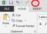
Select the Customize Quick Access Toolbar icon
Click on the arrow show the Quick Access Toolbar menu.
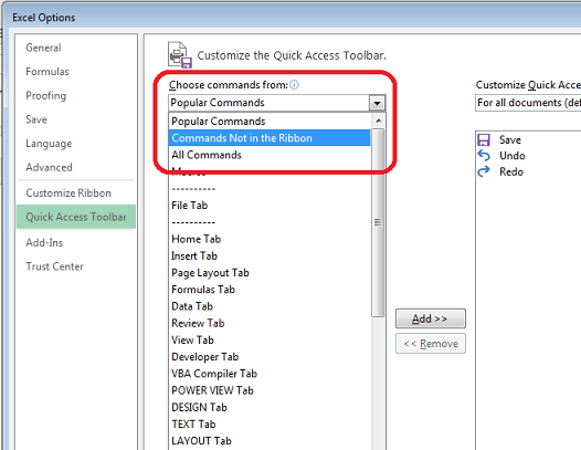
Next click More commands.
Browser Commands not in the toolbar
From the Choose commands from: menu select Commands not in the toolbar.
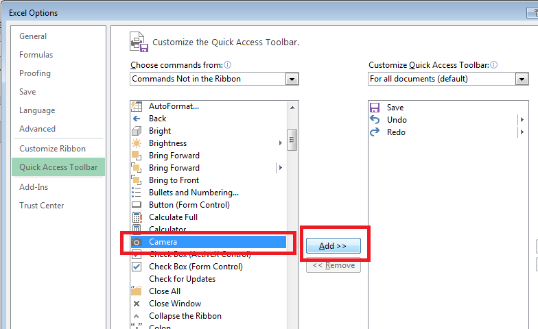
Now you should see an item called Camera in the list of Commands.
Add the Camera Tool
Now select Camera and hit the Add button to add the Camera tool to your Quick Access Toolbar.
Now you should see the Excel Camera Tool Icon in your Quick Access Toolbar:
Use Excel Camera Tool in VBA
The Camera Tool is very useful in your everyday work when you need to copy part of your Workbook as an Image i.e. send an image snapshot of an Excel Worksheet or Chart. Fortunately there is also an easy way to use it in VBA:
Sub TestCamera()
    Dim rng As Range
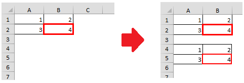
    Set rng = Range("A1:B2")
    'Copy the Picture
    rng.CopyPicture Appearance:=xlScreen, Format:=xlPicture
    'Past the Picture
    Range("A3").PasteSpecial
    Application.CutCopyMode = False
End Sub
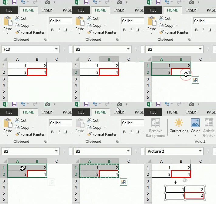
An example of how the macro works below:
Nice huh? Well this is the beginning of things you can do. There are lot of cool ideas you can use this feature to:
- Send image snapshot of Excel Worksheet via Email
- Save Excel Workbook as static image – replace each Worksheet with a static Image to protect your formulas and calculations
Excel Sheet Vector Art
—
259
royalty free vector graphics and clipart matching Excel Sheet
Filters
of 3
Click to view uploads for {{user_display_name}}
{{user_display_name}}
Bookmark icon
Collection
Next Page
of 3
Related Searches
- paper
- sheet
- blank
- stationery
- office supplies
- office
- note
- background
- school supplies
- template
- sheet music
- paper sheet
- sheet music background
- excel
- music sheet
- sheet metal
- spread sheet
- glass sheet
- bed sheet
- calendar sheet
- notebook sheet
paper
sheet
blank
stationery
office supplies
office
note
background
school supplies
template
sheet music
paper sheet


