Ignore all errors excel

Summary:

Our today’s topic will give you the best idea on How To Ignore All Errors In Excel. So that any Excel user can easily handle commonly rendered errors of Excel.

Microsoft Excel is the most popular application of the Microsoft Office suite. This is used in both personal as well as professional life. We can easily manage; organize data, carry out complex calculations, and lots more easily with it.

Undoubtedly this is very important for performing different functions without any hassle. This is the reason Microsoft has provided various functions and features to make the task easy for the users.

However, despite its popularity and advancement, this is not free from errors.

Sometimes while using Excel formulas and functions, result in error values and returns inadvertent results.

So today in this article, I am describing how to handle/ignore all errors in Excel.

How To Trace Error In Excel?

While using the Excel spreadsheet if you entered an incorrect Excel formula or by mistake enter any wrong value, a small green triangle appears in the upper left corner of the cell, near the wrong formula.

But if you get a cryptic three or four letter before the sign (#) in the cell, then this means you are facing any unusual error in Excel.

So, if you encounter any sign among the two, then it is clear you are getting Excel error.

Well, if you want to fix the Excel formulas error, then Relax! As there are certain ways to ignore all errors in Excel.

You need to execute certain rules to check for Excel errors. Checking these rules will help you recognize the issue. But there is no guarantee that your worksheet is error-free.

You can individually turn On or Off any of the rules. The errors can be fixed in two ways:

1. One particular error at a time (spell checker)
2. Or directly as they appear on a worksheet when you type or enter data.

Well, in this way you can fix the error by utilizing the options that Excel displays or else you can even ignore the error by un-checking Ignore Error.

In a specific cell, if you ignore an error, the error in that cell does not appear in additional error checks.

Note: The previously ignored errors can be reset to appear again.

So, check out the following methods to ignore all errors in Excel.

Method 1# Error Checking Options

The Error Checking Options button appears when the formula in the Excel worksheet cell causes an error. Additionally, as I said above the cell itself displays a small green triangle in the upper left corner.

And as you click the button the error type is exhibited, with the list of error checking options.

Well, if you want to ignore the errors completely then simply uncheck the Error Checking option.

Steps to Turn Error Checking Option On/Off

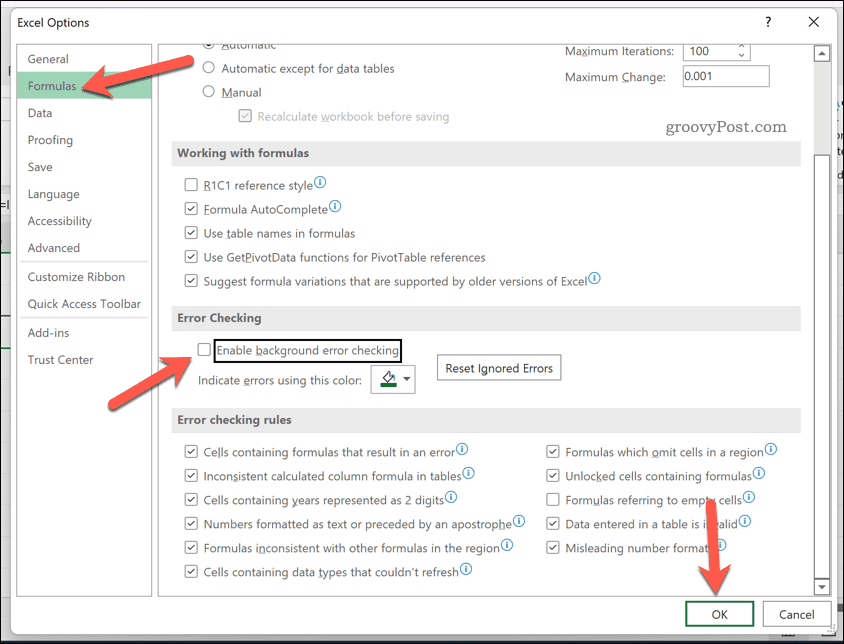
• Click File > Options > Formulas.
• Then under Error Checking, check Enable background error checking. (Doing this mark the error with a triangle in the top-left corner of the cell.)

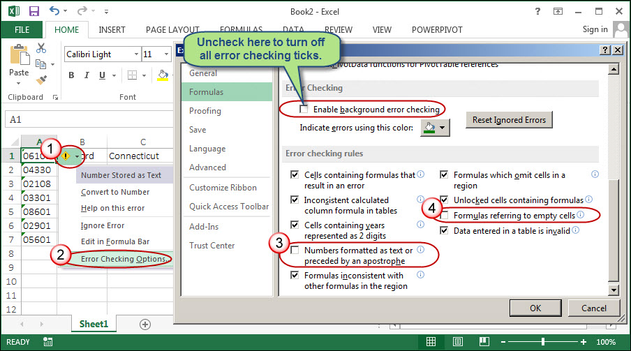
• Also, you can change the color of the triangle marked as an error in the > Indicate errors using this color box > choose the desired color type.
• Now under Excel checking rules > you can check or uncheck the rules boxes that you want.
  • Cells containing formulas that result in an error
  • Inconsistent calculated column formula in tables:
  • Cells containing years represented as 2 digits
  • Numbers formatted as text or preceded by an apostrophe
  • Formulas inconsistent with other formulas in the region
  • Formulas that omit cells in a region
  • Unlocked cells containing formulas
  • Formulas referring to empty cells
  • Data entered in a table is invalid

Method 2# Fix an Inconsistent Formula

While entering the formula in the Excel workbook if get an inconsistent formula then this means the formula in the cell does not match the formula’s pattern.

So here follow the steps to fix it:

• Click Formulas > Show Formulas.
• You will see the formulas in all cells > instead of the calculated results.
• Now compare the inconsistent formula with the one before and after > correct any unintentional inconsistencies.
• As finished > click Formulas > Show Formulas. This will now show the calculated results of all cells
• If it won’t work for you > select a nearby cell nearby that won’t have any issue.
• And click Formulas > Trace Precedents > choose the cell that won’t have any issue.
• Click Formulas > Trace Precedents > compare blue arrows > correct issues with the inconsistent formula.
• Click Formulas > Remove Arrows.

Doing this will help you fix the inconsistent formula error.

Method 3# Hide error values and error indicators

If your Excel formula is having such errors that you don’t need to correct then it’s the best idea to hide it. So, that it won’t appear in your result. Well, this task is possible in Excel by hiding the error indicator and values in cells.

Hide Error Indicators In Cells

If your cell is having a formula that breaks the rule which Excel usually uses for checking up the issues. Then you will see a triangle at the top left corner of the cell. Well, you have the option to hide this indicator from being displayed.

Here is the figure which shows how the Cell appears with the error indicator:

1. Go to the Excel menu and tap the Preferences option.
2. Within the Formulas and Lists, tap to the Error Checking. After then remove the checkmark from the Enable background error checking

Some Other Commonly Encountered Excel Errors Along With The Fixes:

1. VBA Runtime Error 1004

This error is faced by the users while trying to copy/paste the filtered data programmatically in Microsoft Office Excel and in this case you will receive one of the below-given error messages:

• Runtime error 1004: Paste method of worksheet class failed.
• Runtime error 1004: Copy method of Range Class Failed.

One of these error messages appears when the data is pasted into the workbook.

To follow the complete fixes visit: How to Repair Runtime Error 1004 in Excel

2. Excel VLOOKUP Function Not Working

While using the Excel VLOOKUP function getting the #N/A, the error is common. This is faced by the users while trying to match a lookup value within an array. The error commonly shows that the function has failed to locate the lookup value in the lookup array.

To know more about it read: 5 Reasons Behind “Excel VLOOKUP Not Working” Error Occurrence

Automatic Solution: MS Excel Repair Tool

Make use of the professional recommended  MS Excel Repair Tool to repair corrupt, damaged as well as errors in Excel file. This tool allows to easily restore all corrupt Excel files including the charts, worksheet properties cell comments, and other important data. With the help of this, you can fix all sort of issues, corruption, errors in Excel workbooks.

This is a unique tool to repair multiple excel files at one repair cycle and recovers the entire data in a preferred location. It is easy to use and compatible with both Windows as well as Mac operating systems. This supports the entire Excel version and the demo version is free.

* Free version of the product only previews recoverable data.

Steps to Utilize MS Excel Repair Tool:

Conclusion:

Well, this is all about how to ignore all errors in Excel.

There are ways that help you recognize the Excel formulas and function errors in the workbook.

Read the complete article to know more about the errors and ways to handle and ignore errors in Excel.

I tried my best to put together the complete information about the common Excel problems and ways to handle them easily, so implement them and make your Excel workbook error-free.

Additionally, Excel is an essential application and used in daily life, so it is recommended to handle the Excel file properly and follow the best preventive steps to protect your Excel files from getting corrupted.

Despite it, always create a valid backup of your crucial Excel data and as well scan your system with a good antivirus program for virus and malware infection.

If, in case you have any additional questions concerning the ones presented, do tell us in the comments section below or you can also visit our Repair MS Excel social accounts.

Good Luck….

See all How-To Articles

This tutorial demonstrates how to ignore all errors in Excel and Google Sheets.

When working in Excel, you can encounter many different types of errors, and they’re all indicated by a little green triangle in the upper left corner of a cell. This means that a cell contains an error. There are several ways to ignore errors in Excel.

Ignore Error in a Single Cell or Range

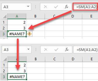
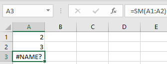
If you have an error in a single cell or in a range of cells, you can ignore them easily. Say that you have the SUM function in cell A3, which sums values from A1 and A2, but you misspelled it as SM.

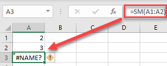
Therefore, cell A3 contains the #NAME? error and the green triangle, instead of the result. To ignore the error and remove the green triangle, (1) click on the yellow icon with the exclamation mark and (2) choose Ignore Error.

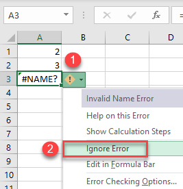
As a result, this cell is no longer marked as an error, and the green triangle has disappeared.

Note: This doesn’t mean that the error is solved, however, it still exists, but Excel is not marking the cell as an error.

Turn Off Error Checking Options

Instead of manually ignoring errors, you can disable error checking options for the whole workbook. To do this, follow the next steps.

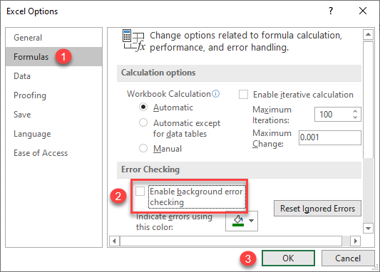
1. In the Ribbon, (1) go to File > Options.

2. In the Excel Options window, (1) go to the Formulas tab, (2) uncheck Enable background error checking, and (3) click OK.

As a result, you won’t get green triangles in cells with formula errors.

Use IFERROR Function

Although previous options hide the green arrow from a cell, the error (#NAME? or similar) is still present in the cell. If you want to avoid displaying the error, you can use the IFERROR function, display a text you want, or keep the cell blank. To do this, you have to nest your formula into the IFERROR function. In cell A3, enter the formula:

=IFERROR(SM(A1:A2),"Formula Error")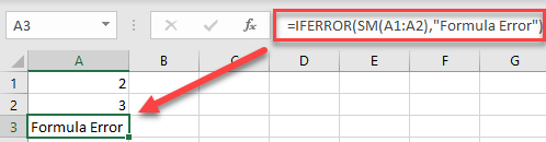

The second argument of the IFERROR function (Formula Error) will be displayed in the cell if the formula in the first argument (SM(A1:A2)) has an error. If not, the result of the formula is displayed.

In Google Sheets, if a formula contains an error, a small red triangle appears in the right upper corner of the cell. There is no option to ignore it as in Excel, but you can use the IFERROR function in the same manner.

An error in Excel is a sign that a calculation or formula has failed to provide a result. You can hide Excel errors in a few different ways. Here’s how.

The perfect Microsoft Excel spreadsheet doesn’t contain errors—or does it?

Excel will throw out an error message when it can’t complete a calculation. There are a number of reasons why, but it’ll be up to you to figure it out and solve it. Not every error can be solved, however.

If you don’t want to fix the problem, or you simply can’t, you can decide to ignore the Excel errors instead. You might decide to do this if the error doesn’t change the results you’re seeing, but you don’t want to see the message.

If you’re unsure how to ignore all errors in Microsoft Excel, follow the steps below.

How to Hide Error Indicators in Excel

Used a formula incorrectly? Rather than return an incorrect result, Excel will throw up an error message. For example, you might see a #DIV/0 error message if you try to divide a value by zero. You may also see other on-screen error indicators, such as warning icons next to the cell containing the error.

You can’t hide the error message without altering the formula or function you’re using but you can hide the error indicator. This will make it less obvious that the spreadsheet data is incorrect.

To quickly hide error indicators in Excel:

1. Open your Excel spreadsheet.
2. Select the cell (or cells) containing the error messages.
3. Click the warning icon that appears next to the cells when selected.
4. From the drop-down, select Ignore Error.
   

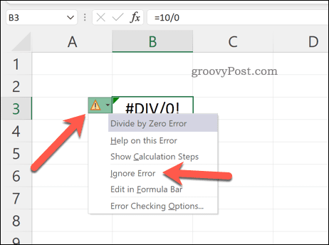
The warning icon will disappear, ensuring the error appears more discreetly in your spreadsheet. If you want to hide the error itself, you’ll need to follow the steps below.

How to Use IFERROR in Excel to Hide Errors

The best way to stop error messages from appearing in Excel is to use the IFERROR function. IFERROR uses IF logic to check a formula before returning a result.

For example, if a cell returns an error, return a value. If it doesn’t return an error, return the correct result. You can use IFERROR to hide error messages and make your Excel spreadsheet error-free (visually, at least).

The structure for an IFERROR formula is =IFERROR(value,value_if_error). You’ll need to replace value with a nested function or calculation that may contain an error. Replace value_if_error with the message or value that Excel should return instead of an error message.

If you’d rather see no error message appearing, use an empty text string (eg. “”) instead.

To use IFERROR in Excel:

1. Open your Excel spreadsheet.
2. Select an empty cell.
3. In the formula bar, type your IFERROR formula (eg. =IFERROR(10/0,””)
4. Press Enter to view the result.
   

IFERROR is a simple but powerful tool for hiding Excel errors. You can nest multiple functions within it, but to test it out, make sure the function you’re using is designed to return an error. If the error doesn’t appear, you’ll know it works.

How to Disable Error Reporting in Excel

If you want to disable error reporting in Excel completely, you can. This ensures that your spreadsheet remains free of errors, but you don’t need to use workarounds like IFERROR to do it.

You might decide to do this to prepare a spreadsheet for printing (even if there are errors). As your data might become incomplete or incorrect with error reporting disabled in Excel, we wouldn’t recommend disabling it for production use.

To disable error reporting in Excel:

1. Open your Excel document.
2. On the ribbon, press File.
   
3. In File, press Options (or More > Options).
   
4. In Excel Options, press Formulas.
5. Uncheck the Enable background error checking checkbox.
6. Press OK to save.
   

Resolving Issues in Microsoft Excel

If you’ve followed the steps above, you should be able to ignore all errors in an Excel spreadsheet. While it isn’t always possible to fix a problem in Excel, you don’t need to see it. IFERROR works well, but if you want a quick fix, you can always disable error reporting entirely.

Excel is a powerful tool, but only if it’s working properly. You may need to troubleshoot further if Excel keeps crashing, but an update or restart will usually fix it.

If you have a Microsoft 365 subscription, you can also try repairing your Office installation. If the file’s at fault, try repairing your document files instead.

A perfectly organized Excel spreadsheet does not have any errors. Do you agree with this statement?

Well, it clearly does not mean that your sheet will not have an error if it is organized manually. Whenever Excel finds any trouble in calculating, you will get an error notification instantly. Why it happens, could have many reasons and each reason has its different solution.

Excel ignore all errors is useful only when you can’t find a fix to the error or you don’t want to solve it. here you will get to know how you can ignore all errors in Excel.

How Do You Find an Error in Excel?

Before getting to know how Excel ignore all errors, let’s understand how you can find an error in Excel. Whenever a wrong formula is typed in Excel or accidentally you put an incorrect value, you will see a little green triangle pops up in the top left side of the cell where the wrong formula is entered.

If three or four letters appear before the sign (#) in the cell, it simply shows that you are about to face an error in Excel. Therefore, be careful whenever you note any sign because it clearly indicates an error.

On the other hand, when you need to fix these errors, you can do it. You can follow simple ways to ignore all errors in Excel.

Error Checking:

In the Error Checking menu, you can check on or off the background error. Apart from that, this menu lets you set the color displays for error indications.

Error Checking Rules:

With the Error Checking Rules menu, you can personalize the error types in Excel checks. This menu can make you able to activate or deactivate several checkboxes that notify errors in Excel.

How does Excel Ignore All Errors with the Shortcut Menu?

Sometimes, you may have to ignore errors in specific cells and for this, you can simply drag the selected cells with a green triangle. Click on the Trace Error option and choose Ignore Error given in the shortcut menu.

This option lets you ignore errors located in the certain cells you have selected. Once you have selected ignore the error, you will not see the green triangle.

How Excel Ignores All Errors?

As you already know that specific rules are followed to check for Excel errors. However, it does not ensure that the worksheet is error-free. You need to manually turn On or Off these rules. You can fix these errors using two ways:

1. One specific error at a time, e.g. spell checker
2. Or directly as they appear on a worksheet when you type data.

That’s how you can fix the error by using this option or else you can ignore the error by un-checking Ignore Error. When you ignore an error in a certain cell, you will not see the error in additional error checks. Also, note that the errors you ignored earlier will be reset as well.

Below is an easy-to-follow method that lets you ignore all errors.

Error Checking Options:

If the formula you have entered is not correct, the Error Checking Options button will appear. Besides, you will also see a green triangle.

Steps to Turn On/Off Error Checking Options

• Open the File menu and choose Options.
• Now, click on Formulas from the menu list.
• Check Enable background error checking option given under the Error Checking.

• Apart from that, you can even make changes in the color of the triangle that indicates errors.
• You can select any color from the Indicate errors with this color box.

Excel checking rules list lets you check or uncheck boxes as per your needs.

• Unlocked cells containing formulas
• Inconsistent calculated column formula in tables
• Formulas inconsistent with other formulas in the region
• Cells with years represented as 2 digits
• Cells with formulas that give an error
• Data entered in a table is invalid
• Formulas refer to blank cells
• Formulas that exclude cells in the region

How You Can Fix an Issue in Excel?

When a user follows the Excel rules perfectly, chances are that he will not have to face any issues while executing a task. Once the above-mentioned steps are followed orderly, Excel ignore all errors is possible. Though fixing an error is not possible always however Excel has a solution to every problem you face while working.

In Excel, to ignore all the errors that you get while using formulas, you can use an error-handling function. You can wrap your original formula with an error-handling function that shows a meaningful result when an error occurs. Other than that, you can use the ignore error option as well that you have in Excel.

In this tutorial, we will look at all those methods that we can use.

Using IFERROR to Ignore Errors and Replace it with a Meaningful Message

The best way to deal with errors is to use the IFERROR function. In this function, you have two arguments to define. The one is the actual value that you need to test for the error and then the value that you want to get if an error occurs.

In the following example, you can see we have used the same formula, but we have wrapped it in the IFERROR and it has returned the value that we have defined.

=IFERROR(1/0,"There's an error.")

IFNA Function to Ignore #N/A Error

If you specifically want to ignore the #N/A error and replace it with a meaningful message, then you can use the IFNA function that only deals with the #N/A. This function also has two arguments that you need to define.

As you can see in the following example, we have the error in cell D1 which comes from the VLOOKUP function.

Now to deal with this error, you can use the IFNA (you can also use IFERROR with the VLOOKUP, but we will use IFNA here).

=IFNA(VLOOKUP("E",A1:B5,2,0),"Value is available.")

Ignoring Error from the Options

When you get an error in a cell, Excel gives you an option along with that cell where you can use the “Ignore Error” option. As you can see in the following example, you have an #DIV/0! error in cell A1.

Now with cell A1, you have a small icon on the right side, and when you click on this icon it further gives a you list of options. And from these options, you can select the “Ignore Error” option.

And once you click on this option, Excel stops marking that cell as an error cell.

Turn ON-OFF Error Checking Options

Apart from that, you can use error-checking options from the Excel options to deal with errors in Excel and ignore them.

When you click on “Error Checking Options”, you get the Excel Options dialog box, from where you can turn on and off the error checking options.

From these options, you need to un-tick the “Enable background error checking” to turn off the error checking options. The moment you do this it will turn off error checking for the entire Excel application.