
The IF function allows you to make a logical comparison between a value and what you expect by testing for a condition and returning a result if that condition is True or False.
-
=IF(Something is True, then do something, otherwise do something else)
But what if you need to test multiple conditions, where let’s say all conditions need to be True or False (AND), or only one condition needs to be True or False (OR), or if you want to check if a condition does NOT meet your criteria? All 3 functions can be used on their own, but it’s much more common to see them paired with IF functions.
Use the IF function along with AND, OR and NOT to perform multiple evaluations if conditions are True or False.
Syntax
-
IF(AND()) — IF(AND(logical1, [logical2], …), value_if_true, [value_if_false]))
-
IF(OR()) — IF(OR(logical1, [logical2], …), value_if_true, [value_if_false]))
-
IF(NOT()) — IF(NOT(logical1), value_if_true, [value_if_false]))
|
Argument name |
Description |
|
|
logical_test (required) |
The condition you want to test. |
|
|
value_if_true (required) |
The value that you want returned if the result of logical_test is TRUE. |
|
|
value_if_false (optional) |
The value that you want returned if the result of logical_test is FALSE. |
|
Here are overviews of how to structure AND, OR and NOT functions individually. When you combine each one of them with an IF statement, they read like this:
-
AND – =IF(AND(Something is True, Something else is True), Value if True, Value if False)
-
OR – =IF(OR(Something is True, Something else is True), Value if True, Value if False)
-
NOT – =IF(NOT(Something is True), Value if True, Value if False)
Examples
Following are examples of some common nested IF(AND()), IF(OR()) and IF(NOT()) statements. The AND and OR functions can support up to 255 individual conditions, but it’s not good practice to use more than a few because complex, nested formulas can get very difficult to build, test and maintain. The NOT function only takes one condition.

Here are the formulas spelled out according to their logic:
|
Formula |
Description |
|---|---|
|
=IF(AND(A2>0,B2<100),TRUE, FALSE) |
IF A2 (25) is greater than 0, AND B2 (75) is less than 100, then return TRUE, otherwise return FALSE. In this case both conditions are true, so TRUE is returned. |
|
=IF(AND(A3=»Red»,B3=»Green»),TRUE,FALSE) |
If A3 (“Blue”) = “Red”, AND B3 (“Green”) equals “Green” then return TRUE, otherwise return FALSE. In this case only the first condition is true, so FALSE is returned. |
|
=IF(OR(A4>0,B4<50),TRUE, FALSE) |
IF A4 (25) is greater than 0, OR B4 (75) is less than 50, then return TRUE, otherwise return FALSE. In this case, only the first condition is TRUE, but since OR only requires one argument to be true the formula returns TRUE. |
|
=IF(OR(A5=»Red»,B5=»Green»),TRUE,FALSE) |
IF A5 (“Blue”) equals “Red”, OR B5 (“Green”) equals “Green” then return TRUE, otherwise return FALSE. In this case, the second argument is True, so the formula returns TRUE. |
|
=IF(NOT(A6>50),TRUE,FALSE) |
IF A6 (25) is NOT greater than 50, then return TRUE, otherwise return FALSE. In this case 25 is not greater than 50, so the formula returns TRUE. |
|
=IF(NOT(A7=»Red»),TRUE,FALSE) |
IF A7 (“Blue”) is NOT equal to “Red”, then return TRUE, otherwise return FALSE. |
Note that all of the examples have a closing parenthesis after their respective conditions are entered. The remaining True/False arguments are then left as part of the outer IF statement. You can also substitute Text or Numeric values for the TRUE/FALSE values to be returned in the examples.
Here are some examples of using AND, OR and NOT to evaluate dates.

Here are the formulas spelled out according to their logic:
|
Formula |
Description |
|---|---|
|
=IF(A2>B2,TRUE,FALSE) |
IF A2 is greater than B2, return TRUE, otherwise return FALSE. 03/12/14 is greater than 01/01/14, so the formula returns TRUE. |
|
=IF(AND(A3>B2,A3<C2),TRUE,FALSE) |
IF A3 is greater than B2 AND A3 is less than C2, return TRUE, otherwise return FALSE. In this case both arguments are true, so the formula returns TRUE. |
|
=IF(OR(A4>B2,A4<B2+60),TRUE,FALSE) |
IF A4 is greater than B2 OR A4 is less than B2 + 60, return TRUE, otherwise return FALSE. In this case the first argument is true, but the second is false. Since OR only needs one of the arguments to be true, the formula returns TRUE. If you use the Evaluate Formula Wizard from the Formula tab you’ll see how Excel evaluates the formula. |
|
=IF(NOT(A5>B2),TRUE,FALSE) |
IF A5 is not greater than B2, then return TRUE, otherwise return FALSE. In this case, A5 is greater than B2, so the formula returns FALSE. |

Using AND, OR and NOT with Conditional Formatting
You can also use AND, OR and NOT to set Conditional Formatting criteria with the formula option. When you do this you can omit the IF function and use AND, OR and NOT on their own.
From the Home tab, click Conditional Formatting > New Rule. Next, select the “Use a formula to determine which cells to format” option, enter your formula and apply the format of your choice.

Using the earlier Dates example, here is what the formulas would be.

|
Formula |
Description |
|---|---|
|
=A2>B2 |
If A2 is greater than B2, format the cell, otherwise do nothing. |
|
=AND(A3>B2,A3<C2) |
If A3 is greater than B2 AND A3 is less than C2, format the cell, otherwise do nothing. |
|
=OR(A4>B2,A4<B2+60) |
If A4 is greater than B2 OR A4 is less than B2 plus 60 (days), then format the cell, otherwise do nothing. |
|
=NOT(A5>B2) |
If A5 is NOT greater than B2, format the cell, otherwise do nothing. In this case A5 is greater than B2, so the result will return FALSE. If you were to change the formula to =NOT(B2>A5) it would return TRUE and the cell would be formatted. |
Note: A common error is to enter your formula into Conditional Formatting without the equals sign (=). If you do this you’ll see that the Conditional Formatting dialog will add the equals sign and quotes to the formula — =»OR(A4>B2,A4<B2+60)», so you’ll need to remove the quotes before the formula will respond properly.
Need more help?

See also
You can always ask an expert in the Excel Tech Community or get support in the Answers community.
Learn how to use nested functions in a formula
IF function
AND function
OR function
NOT function
Overview of formulas in Excel
How to avoid broken formulas
Detect errors in formulas
Keyboard shortcuts in Excel
Logical functions (reference)
Excel functions (alphabetical)
Excel functions (by category)
We use the IF statement in Excel to test one condition and return one value if the condition is met and another if the condition is not met.
However, we use multiple or nested IF statements when evaluating numerous conditions in a specific order to return different results.
This tutorial shows four examples of using nested IF statements in Excel and gives five alternatives to using multiple IF statements in Excel.
General Syntax of Nested IF Statements (Multiple IF Statements)
The general syntax for nested IF statements is as follows:
=IF(Condition1, Value_if_true1, IF(Condition2, Value_if_true2, IF(Condition3, Value_if_true3, Value_if_false)))
This formula tests the first condition; if true, it returns the first value.
If the first condition is false, the formula moves to the second condition and returns the second value if it’s true.
Each subsequent IF function is incorporated into the value_if_false argument of the previous IF function.
This process continues until all conditions have been evaluated, and the formula returns the final value if none of the conditions is true.
The maximum number of nested IF statements allowed in Excel is 64.
Now, look at the following four examples of how to use nested IF statements in Excel.
Example #1: Use Multiple IF Statements to Assign Letter Grades Based on Numeric Scores
Let’s consider the following dataset showing some students’ scores on a Math test.

We want to use nested IF statements to assign student letter grades based on their scores.
We use the following steps:
- Select cell C2 and type in the below formula:
=IF(B2>=90,"A",IF(B2>=80,"B",IF(B2>=70,"C",IF(B2>=60,"D","F"))))

- Click Enter in the cell to get the result of the formula in the cell.
- Copy the formula for the rest of the cells in the column
The assigned letter grades appear in column C.

Explanation of the formula
=IF(B2>=90,”A”,IF(B2>=80,”B”,IF(B2>=70,”C”,IF(B2>=60,”D”,”F”))))
This formula evaluates the value in cell B2 and assigns an “A” if the value is 90 or greater, a “B” if the value is between 80 and 89, a “C” if the value is between 70 and 79, a “D” if the value is between 60 and 69, and an “F” if the value is less than 60.
Notice that it can be challenging to keep track of which parentheses go with which arguments in nested IF functions.
Therefore, as we enter the formula, Excel uses different colors for the parentheses at each level of the nested IF functions to make it easier to see which parts of the formula belong together.

Also read: How to use Excel If Statement with Multiple Conditions Range
Example #2: Use Multiple IF Statements to Calculate Commission Based on Sales Volume
Here’s the dataset showing the sales of specific salespeople in a particular month.

We want to use multiple IF statements to calculate the tiered commission for the salespeople based on their sales volume.
We proceed as follows:
- Select cell C2 and enter the following formula:
=IF(B2>=40000, B2*0.14,IF(B2>=20000,B2*0.12,IF(B2>=10000,B2*0.105,IF(B2>0,B2*0.08,0))))

- Press the Enter key to get the result of the formula.
- Double-click or drag the Fill Handle to copy the formula down the column.
The commission for each salesperson is displayed in column D.

Explanation of the formula
=IF(B2>=40000, B2*0.14,IF(B2>=20000,B2*0.12,IF(B2>=10000,B2*0.105,IF(B2>0,B2*0.08,0))))
This formula evaluates the value in cell B2 and then does the following:
- If the value in cell B2 is greater than or equal to 40,000, the figure is multiplied by 14% (0.14).
- If the figure in cell B2 is less than 40,000 but greater than or equal to 20,000, the value is multiplied by 12% (0.12).
- If the number in cell B2 is less than 20,000 but greater than or equal to 10,000, the figure is multiplied by 10.5% (0.105).
- If the value in cell B2 is less than 10,000 but greater than 0 (zero), the number is multiplied by 8% (0.08).
- If the value in cell B2 is 0 (zero), 0 (zero) is returned.
Example #3: Use Multiple IF Statements to Assign Sales Performance Rating Based On Sales Target Achievement
The following is a dataset showing regional sales data of a specific technology company in a particular year.

We want to use multiple IF statements to assign a sales performance rating to each region based on their sales target achievement.
We use the following steps:
- Select cell C2 and type in the below formula:
=IF(B2>500000, "Excellent", IF(B2>400000, "Good", IF(B2>275000, "Average", "Poor")))

- Click Enter on the Formula bar.
- Drag or double-click the Fill Handle to copy the formula down the column.
The performance ratings of the regions are shown in column C.

Explanation of the formula
=IF(B2>500000, “Excellent”, IF(B2>400000, “Good”, IF(B2>275000, “Average”, “Poor”)))
In this formula, if the sales target in cell B2 is greater than 500,000, the formula returns “Excellent.”
If it’s between 400,000 and 500,000, the formula returns “Good.”
If it’s between 275,000 and 400,000, the formula returns “Average.” And if it’s below 275,000, the formula returns “Poor.”
Example #4: Use Multiple IF Statements in Excel to Check For Errors and Return Error Messages
Suppose we have the following dataset of students’ English test scores. Some scores are less than 0 or greater than 100, and there are no scores in some cases.

We want to use nested IF statements to check for scores in column B and display error messages in column C if there are no scores or the scores are less than 0 or greater than 100.
If the score in column B is valid, we want the formula to return an empty string in column C.
Here are the steps to follow:
- Select cell C2 and enter the following formula:
=IF(OR(B2<0,B2>100),"Score out of range",IF(ISBLANK(B2),"Invalid score",""))

- Click Enter on the Formula bar.
- Drag the Fill Handle to copy the formula down the column.
The error messages are shown in column C.

Explanation of the formula
=IF(OR(B2<0,B2>100),”Score out of range”,IF(ISBLANK(B2),”Invalid score”,””))
This formula uses the OR function to check if the score in cell B2 is less than 0 or greater than 100, and if it is, it returns the error message “Score out of range.”
The formula also uses the ISBLANK function to check if cell B2 is blank, and if it is, it returns the error message “Invalid score.”
If there is no error, the formula returns an empty string, meaning no message is displayed in column B.
Alternatives to Using Multiple IF Statements in Excel
Formulas using nested IF statements can become difficult to read and manage if we have more than a few conditions to test.
In addition, if we exceed the maximum allowed limit of 64 nested IF statements, we will get an error message.
Fortunately, Excel offers alternative ways to use instead of nested IF functions, especially when we need to test more than a few conditions.
We present the alternative ways in this tutorial.
Alternative #1: Use the IFS Function
The IFS function tests whether one or more conditions are met and returns a value corresponding to the first TRUE condition.
Before the release of the IFS function in 2018 as part of the Excel 365 update, the only way to test multiple conditions and return a corresponding value in Excel was to use nested IF statements.
However, multiple IF statements have the downside of resulting in unwieldy formulas that are difficult to read and maintain.
In some situations, the IFS function is designed to replace the need for multiple IF functions.
The syntax of the IFS function is more straightforward and easier to read than nested IF statements, and it can handle up to 127 conditions.
Here’s an example:
Let’s consider the following dataset showing some students’ scores on a Math test.

We want to use the IFS function to assign letter grades to the students based on their scores.
We use the following steps:
- Select cell C2 and type in the below formula:
=IFS(B2>=90, "A", B2>=80, "B", B2>=70, "C", B2>=60, "D", B2<60, "F")

- Click Enter on the Formula bar.
- Drag or double-click the Fill Handle to copy the formula down the column.
The student’s letter grades are shown in column C.

Explanation of the formula
=IFS(B2>=90, “A”, B2>=80, “B”, B2>=70, “C”, B2>=60, “D”, B2<60, “F”)
This formula tests the score in cell B2 against each condition and returns the corresponding grade letter when the condition is true.
Limitation of IFS Function
The IFS function in Excel is designed to simplify complex nested IF statements.
However, there are situations where the IFS function may not be able to replace nested IF functions completely.
One such situation is when you must calculate or operate based on a condition or set of conditions.
While the IFS function can return a value or text string based on a condition, it cannot perform calculations or operations on that value like nested IF statements.
Another situation where the IFS function may be less useful is when you need to test for a range of conditions rather than just a specific set.
This is because the IFS function requires you to specify each condition and corresponding result separately, which can become cumbersome if you have many conditions to test—in contrast, nested IF statements allow you to test for a range of conditions using logical operators like AND and OR.
The IFS function is a powerful tool for simplifying complex logical tests in Excel.
However, there may be situations where nested IF statements are more appropriate for your needs.
We recommend that you consider both options and choose the one that best fits the specific requirements of your task.
Alternative #2: Use Nested IF Functions
We can use multiple IFS functions in a formula if we have more than one condition to test.
For example, let’s say we have the following dataset of student names and scores on a Physics test in columns A and B.

We want to assign a letter grade to each score and include a pass or fail designation based on whether the score is above or below 75.
Here are the steps to use:
- Select cell C2 and enter the following formula
=IFS(B2>=90,"A",B2>=80,"B",B2>=70,"C",B2>=60,"D",B2<60,"F")&" "&IFS(B2>=75,"Pass",B2<75,"Fail")

- Click Enter on the Formula bar.
- Drag or double-click the Fill Handle to copy the formula down the column.
The letter grade and designation of the student scores are displayed in column C.

Explanation of the formula
=IFS(B2>=90,”A”,B2>=80,”B”,B2>=70,”C”,B2>=60,”D”,B2<60,”F”)&” “&IFS(B2>=75,”Pass”,B2<75,”Fail”)
This formula uses the first IFS function to assign a letter grade based on the score in column A and the second IFS function to give a pass/fail designation based on the score in column A.
The two IFS functions are combined using the ampersand (&) operator to create a single text string that displays each score’s letter grade and pass/fail designation.
Alternative #3: Use the Combination of CHOOSE and XMATCH Functions
The CHOOSE function selects a value or action from a value list based on an index number.
The XMATCH function locates and returns the relative position of an item in an array. We can combine these functions in a formula instead of nested IF functions.
Here’s an example:
Suppose we have the following dataset showing some students’ scores and letter grades on a Biology test.

We want to use a formula combining the CHOOSE and XMATCH functions to assign corresponding grade points in column D to each letter grade.
We use the following steps:
- Select cell D2 and type in the below formula:
=CHOOSE(XMATCH(C2,{"F","E","D","C","B","A"},0),0,1,2,3,4,5)

- Click Enter on the Formula bar.
- Drag or double-click the Fill Handle to copy the formula down the column.
The grade points for each student are displayed in column D.

Explanation of the formula
=CHOOSE(XMATCH(C2,{“F”,”E”,”D”,”C”,”B”,”A”},0),0,1,2,3,4,5)
This formula applies the XMATCH function to find the position of the letter grade in the array {“F”,”E”,”D”,”C”,”B”,”A”}, and then uses the CHOOSE function to return the corresponding grade points.
Alternative #4: Use the VLOOKUP Function
The VLOOKUP function looks for a value in the leftmost column of a table and then returns a value in the same row from a specified column.
We can use the VLOOKUP function instead of nested IF functions in Excel.
The following is an example of using the VLOOKUP function instead of nested IF functions in Excel:
Suppose we have the following dataset showing some students’ scores and letter grades on a Biology test.

We want to use the VLOOKUP function to assign grade points to each student’s letter grade in column D.
We use the steps below:
- Create a table that lists the grades and their corresponding grade points in cell range F1:G7.

- In cell D2, type the following formula:
=VLOOKUP(C2,$F$2:$G$7,2,FALSE)
Note: Use the dollar signs to lock down the cell range F2:G7.

- Click Enter on the Formula bar.
- Drag or double-click the Fill Handle to copy the formula down the column.
The grade points for each student appear in column D.

Explanation of the formula
=VLOOKUP(C2,$F$2:$G$7,2,FALSE)
This formula uses the VLOOKUP function to look up the grade in cell C2 in the table in F2:G7 and return the corresponding grade point in the second column (i.e., column G).
The “FALSE” argument ensures that an exact match is required.
Alternative #5: Use a User-Defined Function
If you need to test more than a few conditions, consider creating a User Defined Function in VBA that can handle many conditions.
Here’s an example of using VBA code to replace nested IF functions in Excel:
Suppose we have the following dataset showing the sales of specific salespeople in a particular month.

We want to use a User Defined Function to calculate the commission for each salesperson based on the following rates:
- If the total sales are less than $10,000, the commission rate is 8%.
- If the total sales are equal to or greater than $10,000 but less than $20,000, the commission rate is 10.5%.
- If the total sales are equal to or greater than $20,000 but less than $40,000, the commission rate is 12%.
- If the sales are equal to or greater than $40,000, the commission rate is 14%
We use the following steps:
- Open the worksheet containing the sales dataset.
- Press Alt + F11 to launch the Visual Basic Editor.
- Click Insert on the menu bar and choose Module to insert a new module.

- Enter the following VBA code.
'Code developed by Steve Scott from https://spreadsheetplanet.com
Function COMMISSION(Sales As Double) As Double
    Const Rate1 = 0.08
    Const Rate2 = 0.105
    Const Rate3 = 0.12
    Const Rate4 = 0.14

'Calculate sales commissions

    Select Case Sales
        Case 0 To 9999.99: COMMISSION = Sales * Rate1
        Case 10000 To 19999.99: COMMISSION = Sales * Rate2
        Case 20000 To 39999.99: COMMISSION = Sales * Rate3
        Case Is >= 40000: COMMISSION = Sales * Rate4
    End Select

End Function
- Save the function procedure and the workbook as a Macro-Enabled Workbook.
- Press Alt + F11 to switch to the active worksheet with the sales dataset.
- Select cell C2 and enter the following formula:
=COMMISSION(B2)

- Click Enter on the Formula bar.
- Drag or double-click the Fill Handle to copy the formula down the column.
The commission for each salesperson is displayed in column C.

This VBA function takes the sales amount as an argument and returns the corresponding commission.
The User-Defined Function is a much simpler and easier-to-read solution than using nested IF functions.
This tutorial showed four examples of using nested IF statements in Excel and gave five alternatives to using multiple IF statements in Excel. We hope you found the tutorial helpful.
Other Excel tutorials you may find useful:
- Excel Logical Test Using Multiple If Statements in Excel [AND/OR]
- How to Compare Two Columns in Excel (using VLOOKUP & IF)
- Using IF Function with Dates in Excel (Easy Examples)
- COUNTIF Greater Than Zero in Excel
- BETWEEN Formula in Excel (Using IF Function) – Examples
- Count Cells Less than a Value in Excel (COUNTIF Less)
Содержание
- IF function – nested formulas and avoiding pitfalls
- Remarks
- Examples
- Additional examples
- Did you know?
- Need more help?
- IFS function
- Simple syntax
- Example 1
- Example 2
- Remarks
- Need more help?
- Функции Excel ЕСЛИ (IF) и ЕСЛИМН (IFS) для нескольких условий
- Функция ЕСЛИ в Excel
- Формула ЕСЛИ в Excel – примеры нескольких условий
IF function – nested formulas and avoiding pitfalls
The IF function allows you to make a logical comparison between a value and what you expect by testing for a condition and returning a result if True or False.
=IF(Something is True, then do something, otherwise do something else)
So an IF statement can have two results. The first result is if your comparison is True, the second if your comparison is False.
IF statements are incredibly robust, and form the basis of many spreadsheet models, but they are also the root cause of many spreadsheet issues. Ideally, an IF statement should apply to minimal conditions, such as Male/Female, Yes/No/Maybe, to name a few, but sometimes you might need to evaluate more complex scenarios that require nesting* more than 3 IF functions together.
* “Nesting” refers to the practice of joining multiple functions together in one formula.
Use the IF function, one of the logical functions, to return one value if a condition is true and another value if it’s false.
IF(logical_test, value_if_true, [value_if_false])
The condition you want to test.
The value that you want returned if the result of logical_test is TRUE.
The value that you want returned if the result of logical_test is FALSE.
While Excel will allow you to nest up to 64 different IF functions, it’s not at all advisable to do so. Why?
Multiple IF statements require a great deal of thought to build correctly and make sure that their logic can calculate correctly through each condition all the way to the end. If you don’t nest your formula 100% accurately, then it might work 75% of the time, but return unexpected results 25% of the time. Unfortunately, the odds of you catching the 25% are slim.
Multiple IF statements can become incredibly difficult to maintain, especially when you come back some time later and try to figure out what you, or worse someone else, was trying to do.
If you find yourself with an IF statement that just seems to keep growing with no end in sight, it’s time to put down the mouse and rethink your strategy.
Let’s look at how to properly create a complex nested IF statement using multiple IFs, and when to recognize that it’s time to use another tool in your Excel arsenal.
Examples
Following is an example of a relatively standard nested IF statement to convert student test scores to their letter grade equivalent.
 97,»A+»,IF(B2>93,»A»,IF(B2>89,»A-«,IF(B2>87,»B+»,IF(B2>83,»B»,IF(B2>79,»B-«,IF(B2>77,»C+»,IF(B2>73,»C»,IF(B2>69,»C-«,IF(B2>57,»D+»,IF(B2>53,»D»,IF(B2>49,»D-«,»F»))))))))))))» loading=»lazy»>
This complex nested IF statement follows a straightforward logic:
If the Test Score (in cell D2) is greater than 89, then the student gets an A
If the Test Score is greater than 79, then the student gets a B
If the Test Score is greater than 69, then the student gets a C
If the Test Score is greater than 59, then the student gets a D
Otherwise the student gets an F
This particular example is relatively safe because it’s not likely that the correlation between test scores and letter grades will change, so it won’t require much maintenance. But here’s a thought – what if you need to segment the grades between A+, A and A- (and so on)? Now your four condition IF statement needs to be rewritten to have 12 conditions! Here’s what your formula would look like now:
It’s still functionally accurate and will work as expected, but it takes a long time to write and longer to test to make sure it does what you want. Another glaring issue is that you’ve had to enter the scores and equivalent letter grades by hand. What are the odds that you’ll accidentally have a typo? Now imagine trying to do this 64 times with more complex conditions! Sure, it’s possible, but do you really want to subject yourself to this kind of effort and probable errors that will be really hard to spot?
Tip: Every function in Excel requires an opening and closing parenthesis (). Excel will try to help you figure out what goes where by coloring different parts of your formula when you’re editing it. For instance, if you were to edit the above formula, as you move the cursor past each of the ending parentheses “)”, its corresponding opening parenthesis will turn the same color. This can be especially useful in complex nested formulas when you’re trying to figure out if you have enough matching parentheses.
Additional examples
Following is a very common example of calculating Sales Commission based on levels of Revenue achievement.
 15000,20%,IF(C9>12500,17.5%,IF(C9>10000,15%,IF(C9>7500,12.5%,IF(C9>5000,10%,0)))))» loading=»lazy»>
This formula says IF(C9 is Greater Than 15,000 then return 20%, IF(C9 is Greater Than 12,500 then return 17.5%, and so on.
While it’s remarkably similar to the earlier Grades example, this formula is a great example of how difficult it can be to maintain large IF statements – what would you need to do if your organization decided to add new compensation levels and possibly even change the existing dollar or percentage values? You’d have a lot of work on your hands!
Tip: You can insert line breaks in the formula bar to make long formulas easier to read. Just press ALT+ENTER before the text you want to wrap to a new line.
Here is an example of the commission scenario with the logic out of order:
 5000,10%,IF(C9>7500,12.5%,IF(C9>10000,15%,IF(C9>12500,17.5%,IF(C9>15000,20%,0)))))» loading=»lazy»>
Can you see what’s wrong? Compare the order of the Revenue comparisons to the previous example. Which way is this one going? That’s right, it’s going from bottom up ($5,000 to $15,000), not the other way around. But why should that be such a big deal? It’s a big deal because the formula can’t pass the first evaluation for any value over $5,000. Let’s say you’ve got $12,500 in revenue – the IF statement will return 10% because it is greater than $5,000, and it will stop there. This can be incredibly problematic because in a lot of situations these types of errors go unnoticed until they’ve had a negative impact. So knowing that there are some serious pitfalls with complex nested IF statements, what can you do? In most cases, you can use the VLOOKUP function instead of building a complex formula with the IF function. Using VLOOKUP, you first need to create a reference table:

This formula says to look for the value in C2 in the range C5:C17. If the value is found, then return the corresponding value from the same row in column D.

Similarly, this formula looks for the value in cell B9 in the range B2:B22. If the value is found, then return the corresponding value from the same row in column C.
Note: Both of these VLOOKUPs use the TRUE argument at the end of the formulas, meaning we want them to look for an approxiate match. In other words, it will match the exact values in the lookup table, as well as any values that fall between them. In this case the lookup tables need to be sorted in Ascending order, from smallest to largest.
VLOOKUP is covered in much more detail here, but this is sure a lot simpler than a 12-level, complex nested IF statement! There are other less obvious benefits as well:
VLOOKUP reference tables are right out in the open and easy to see.
Table values can be easily updated and you never have to touch the formula if your conditions change.
If you don’t want people to see or interfere with your reference table, just put it on another worksheet.
Did you know?
There is now an IFS function that can replace multiple, nested IF statements with a single function. So instead of our initial grades example, which has 4 nested IF functions:
It can be made much simpler with a single IFS function:
The IFS function is great because you don’t need to worry about all of those IF statements and parentheses.
Note: This feature is only available if you have a Microsoft 365 subscription. If you are a Microsoft 365subscriber, make sure you have the latest version of Office.
Need more help?
You can always ask an expert in the Excel Tech Community or get support in the Answers community.
Источник
IFS function
The IFS function checks whether one or more conditions are met, and returns a value that corresponds to the first TRUE condition. IFS can take the place of multiple nested IF statements, and is much easier to read with multiple conditions.
Note: This feature is available on Windows or Mac if you have Office 2019, or if you have a Microsoft 365 subscription. If you are a Microsoft 365 subscriber, make sure you have the latest version.
Simple syntax
Generally, the syntax for the IFS function is:
=IFS([Something is True1, Value if True1,Something is True2,Value if True2,Something is True3,Value if True3)
Please note that the IFS function allows you to test up to 127 different conditions. However, we don’t recommend nesting too many conditions with IF or IFS statements. This is because multiple conditions need to be entered in the correct order, and can be very difficult to build, test and update.
IFS(logical_test1, value_if_true1, [logical_test2, value_if_true2], [logical_test3, value_if_true3],…)
Condition that evaluates to TRUE or FALSE.
Result to be returned if logical_test1 evaluates to TRUE. Can be empty.
Condition that evaluates to TRUE or FALSE.
Result to be returned if logical_testN evaluates to TRUE. Each value_if_trueN corresponds with a condition logical_testN. Can be empty.
Example 1
The formula for cells A2:A6 is:
Which says IF(A2 is Greater Than 89, then return a «A», IF A2 is Greater Than 79, then return a «B», and so on and for all other values less than 59, return an «F»).
Example 2
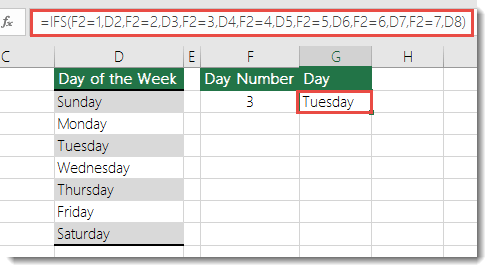
The formula in cell G7 is:
Which says IF(the value in cell F2 equals 1, then return the value in cell D2, IF the value in cell F2 equals 2, then return the value in cell D3, and so on, finally ending with the value in cell D8 if none of the other conditions are met).
To specify a default result, enter TRUE for your final logical_test argument. If none of the other conditions are met, the corresponding value will be returned. In Example 1, rows 6 and 7 (with the 58 grade) demonstrate this.
If a logical_test argument is supplied without a corresponding value_if_true, this function shows a «You’ve entered too few arguments for this function» error message.
If a logical_test argument is evaluated and resolves to a value other than TRUE or FALSE, this function returns a #VALUE! error.
If no TRUE conditions are found, this function returns #N/A error.
Need more help?
You can always ask an expert in the Excel Tech Community or get support in the Answers community.
Источник
Функции Excel ЕСЛИ (IF) и ЕСЛИМН (IFS) для нескольких условий
Логическая функция ЕСЛИ в Экселе – одна из самых востребованных. Она возвращает результат (значение или другую формулу) в зависимости от условия.
Функция ЕСЛИ в Excel
Функция имеет следующий синтаксис.
ЕСЛИ(лог_выражение; значение_если_истина; [значение_если_ложь])
лог_выражение – это проверяемое условие. Например, A2 30) не выполняется и возвращается альтернативное значение, указанное в третьем поле. В этом вся суть функции ЕСЛИ. Протягивая расчет вниз, получаем результат по каждому товару.
Однако это был демонстрационный пример. Чаще формулу Эксель ЕСЛИ используют для более сложных проверок. Допустим, есть средненедельные продажи товаров и их остатки на текущий момент. Закупщику нужно сделать прогноз остатков через 2 недели. Для этого нужно от текущих запасов отнять удвоенные средненедельные продажи.

Пока все логично, но смущают минусы. Разве бывают отрицательные остатки? Нет, конечно. Запасы не могут быть ниже нуля. Чтобы прогноз был корректным, нужно отрицательные значения заменить нулями. Здесь отлично поможет формула ЕСЛИ. Она будет проверять полученное по прогнозу значение и если оно окажется меньше нуля, то принудительно выдаст ответ 0, в противном случае — результат расчета, т.е. некоторое положительное число. В общем, та же логика, только вместо значений используем формулу в качестве условия.

В прогнозе запасов больше нет отрицательных значений, что в целом очень неплохо.
Формулы Excel ЕСЛИ также активно используют в формулах массивов. Здесь мы не будем далеко углубляться. Заинтересованным рекомендую прочитать статью о том, как рассчитать максимальное и минимальное значение по условию. Правда, расчет в той статье более не актуален, т.к. в Excel 2016 появились функции МИНЕСЛИ и МАКСЕСЛИ. Но для примера очень полезно ознакомиться – пригодится в другой ситуации.
Формула ЕСЛИ в Excel – примеры нескольких условий
Довольно часто количество возможных условий не 2 (проверяемое и альтернативное), а 3, 4 и более. В этом случае также можно использовать функцию ЕСЛИ, но теперь ее придется вкладывать друг в друга, указывая все условия по очереди. Рассмотрим следующий пример.
Нескольким менеджерам по продажам нужно начислить премию в зависимости от выполнения плана продаж. Система мотивации следующая. Если план выполнен менее, чем на 90%, то премия не полагается, если от 90% до 95% — премия 10%, от 95% до 100% — премия 20% и если план перевыполнен, то 30%. Как видно здесь 4 варианта. Чтобы их указать в одной формуле потребуется следующая логическая структура. Если выполняется первое условие, то наступает первый вариант, в противном случае, если выполняется второе условие, то наступает второй вариант, в противном случае если… и т.д. Количество условий может быть довольно большим. В конце формулы указывается последний альтернативный вариант, для которого не выполняется ни одно из перечисленных ранее условий (как третье поле в обычной формуле ЕСЛИ). В итоге формула имеет следующий вид.

Комбинация функций ЕСЛИ работает так, что при выполнении какого-либо указанно условия следующие уже не проверяются. Поэтому важно их указать в правильной последовательности. Если бы мы начали проверку с B2 =1. Однако этого можно избежать, если в поле с условием написать ИСТИНА, указывая тем самым, что, если не выполняются ранее перечисленные условия, наступает ИСТИНА и возвращается последнее альтернативное значение.
Теперь вы знаете, как пользоваться функцией ЕСЛИ в Excel, а также ее более современным вариантом для множества условий ЕСЛИМН.
Источник
Excel IF AND OR functions on their own aren’t very exciting, but mix them up with the IF Statement and you’ve got yourself a formula that’s much more powerful.
In this tutorial we’re going to take a look at the basics of the AND and OR functions and then put them to work with an IF Statement. If you aren’t familiar with IF Statements, click here to read that tutorial first.
IF Formula Builder
Our IF Formula Builder does the hard work of creating IF formulas.
You just need to enter a few pieces of information, and the workbook creates the formula for you.
AND Function
The AND function belongs to the logic family of formulas, along with IF, OR and a few others. It’s useful when you have multiple conditions that must be met.
In Excel language on its own the AND formula reads like this:
=AND(logical1,[logical2]....)
Now to translate into English:
=AND(is condition 1 true, AND condition 2 true (add more conditions if you want)
OR Function
The OR function is useful when you are happy if one, OR another condition is met.
In Excel language on its own the OR formula reads like this:
=OR(logical1,[logical2]....)
Now to translate into English:
=OR(is condition 1 true, OR condition 2 true (add more conditions if you want)
See, I did say they weren’t very exciting, but let’s mix them up with IF and put AND and OR to work.
IF AND Formula
First let’s set the scene of our challenge for the IF, AND formula:
In our spreadsheet below we want to calculate a bonus to pay the children’s TV personalities listed. The rules, as devised by my 4 year old son, are:
1) If the TV personality is Popular AND
2) If they earn less than $100k per year they get a 10% bonus (my 4 year old will write them an IOU, he’s good for it though).

In cell D2 we will enter our IF AND formula as follows:
In English first
=IF(Spider Man is Popular, AND he earns <$100k), calculate his salary x 10%, if not put "Nil" in the cell)
Now in Excel’s language:
=IF(AND(B2="Yes",C2<100),C2x$H$1,"Nil")
You’ll notice that the two conditions are typed in first, and then the outcomes are entered. You can have more than two conditions; in fact you can have up to 30 by simply separating each condition with a comma (see warning below about going overboard with this though).
IF OR Formula
Again let’s set the scene of our challenge for the IF, OR formula:
The revised rules, as devised by my 4 year old son, are:
1) If the TV personality is Popular OR
2) If they earn less than $100k per year they get a 10% bonus.

In cell D2 we will enter our IF OR formula as follows:
In English first
=IF(Spider Man is Popular, OR he earns <$100k), calculate his salary x 10%, if not put “Nil” in the cell)
Now in Excel’s language:
=IF(OR(B2="Yes",C2<100),C2x$H$1,"Nil")
Notice how a subtle change from the AND function to the OR function has a significant impact on the bonus figure.
Just like the AND function, you can have up to 30 OR conditions nested in the one formula, again just separate each condition with a comma.
Try other operators
You can set your conditions to test for specific text, as I have done in this example with B2=»Yes», just put the text you want to check between inverted comas “ ”.
Alternatively you can test for a number and because the AND and OR functions belong to the logic family, you can employ different tests other than the less than (<) operator used in the examples above.
Other operators you could use are:
- = Equal to
- > Greater Than
- <= Less than or equal to
- >= Greater than or equal to
- <> Less than or greater than
Warning: Don’t go overboard with nesting IF, AND, and OR’s, as it will be painful to decipher if you or someone else ever needs to update the formula in months or years to come.
Note: These formulas work in all versions of Excel, however versions pre Excel 2007 are limited to 7 nested IF’s.
Download the Workbook
Enter your email address below to download the sample workbook.
By submitting your email address you agree that we can email you our Excel newsletter.
Excel IF AND OR Practice Questions
IF AND Formula Practice
In the embedded Excel workbook below insert a formula (in the grey cells in column E), that returns the text ‘Yes’, when a product SKU should be reordered, based on the following criteria:
- If Stock on hand is less than 20,000 AND
- Demand level is ‘High’
If the above conditions are met, return ‘Yes’, otherwise, return ‘No’.
Tips for working with the embedded workbook:
- Use arrow keys to move around the worksheet when you can’t click on the cells with your mouse
- Use shortcut keys CTRL+C to copy and CTRL+V to paste
- Don’t forget to absolute cell references where applicable
- Do not enter anything in column F
- Double click to edit a cell
- Refresh the page to reset the embedded workbook
IF OR Formula Practice
In the embedded Excel workbook below insert a formula (in the grey cells in column E) that calculates the bonus due for each salesperson. A $500 bonus is paid if a salesperson meets either target in cells C24 and C25, otherwise they earn $0 bonus.
Want More Excel Formulas
Why not visit our list of Excel formulas. You’ll find a huge range all explained in plain English, plus PivotTables and other Excel tools and tricks. Enjoy 🙂
Home > Live Classes > Logical Functions in Excel (IF, IFS, AND, OR, COUNTIF, SUMIF)
In this Excel tutorial, we take a look at Logical Functions in Excel. That’s functions such as IF, IFS, COUNTIF and SUMIF. This is an Excel tutorial for beginners or those who need to brush up on their Excel. This was taken from a live, recorded session. You can download the Excel files that Debs uses below the video and follow along.
Download WorkBook HERE
Once again this was a brilliant live session. Logical functions in Excel are incredibly useful and once you get your head around them, simple to use. In this session we covered:
- The IF Function
- Nested IF in Excel
- The IFS Function
- The AND and OR Functions
- COUNTIF and SUMIF
- Error checking Functions IFERROR and IFNA
To learn all about the more advanced versions of some of these functions, take a look at these tutorials on COUNTIFS, and SUMIFS.
Other Excel classes you might like:
- Introduction to Power Pivot & Power Query in Excel
- What-If Analysis in Excel
- Designing Better Spreadsheets in Excel
Take a look at more recorded live classes from Simon Sez IT.
Adam Lacey

Adam Lacey is an Excel enthusiast and online learning expert. He combines these two passions at Simon Sez IT where he wears a number of different hats.When Adam isn’t fretting about site traffic or Pivot Tables, you’ll find him on the tennis court or in the kitchen cooking up a storm.