If with range of values in excel

To perform complicated and powerful data analysis, you need to test various conditions at a single point in time. The data analysis might require logical tests also within these multiple conditions.

For this, you need to perform Excel if statement with multiple conditions or ranges that include various If functions in a single formula.

Those who use Excel daily are well versed with Excel If statement as it is one of the most-used formula. Here you can check various Excel If or statement, Nested If, AND function, Excel IF statements, and how to use them. We have also provided a VIDEO TUTORIAL for different If Statements.

There are various If statements available in Excel. You have to know which of the Excel If you will work at what condition. Here you can check multiple conditions where you can use Excel If statement.

1) Excel If Statement

If you want to test a condition to get two outcomes then you can use this Excel If statement.

=If(Marks>=40, “Pass”)

2) Nested If Statement

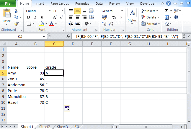
Let’s take an example that met the below-mentioned condition

• If the score is between 0 to 60, then Grade F
• If the score is between 61 to 70, then Grade D
• If the score is between 71 to 80, then Grade C
• If the score is between 81 to 90, then Grade B
• If the score is between 91 to 100, then Grade A

Then to test the condition the syntax of the formula becomes,

=If(B5<60, “F”,If(B5<71, “D”, If(B5<81,”C”,If(B5<91,”B”,”A”)

3) Excel If with Logical Test

There are 2 different types of conditions AND and OR. You can use the IF statement in excel between two values in both these conditions to perform the logical test.

AND Function: If you are performing the logical test based on AND function, then excel will give you TRUE as an outcome in every condition else it will return false.

OR Function: If you are using OR condition for the logical test, then excel will give you an outcome as TRUE if any of the situations match else it returns false.

For this, multiple testing is to be done using AND and OR function, you should gain expertise in using either or both of these with IF statement. Here we have used if the function with 3 conditions.

How to apply IF & AND function in Excel

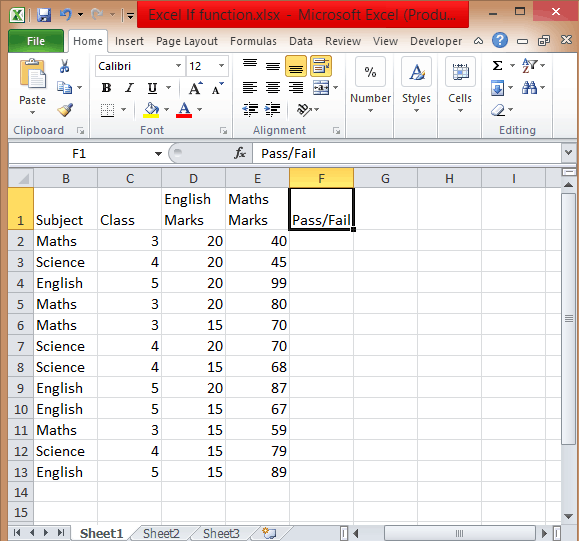
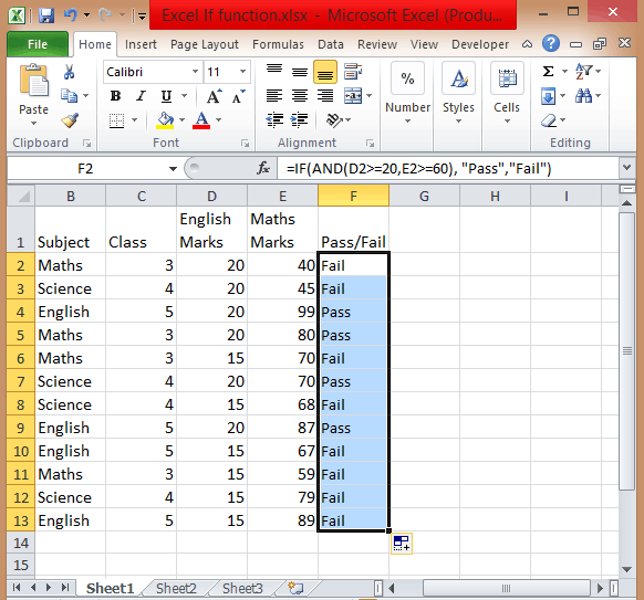
• To perform this multiple if and statements in excel, we will take the data set for the student’s marks that contain fields such as English and Math’s Marks.
• The score of the English subject is stored in the D column whereas the Maths score is stored in column E.
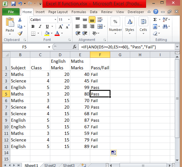
• Let say a student passes the class if his or her score in English is greater than or equal to 20 and he or she scores more than 60 in Maths.
• To create a report in matters of seconds, if formula combined with AND can suffice.
• Type =IF( Excel will display the logical hint just below the cell F2. The parameters of this function are logical_test, value_if_true, value_if_false.
• The first parameter contains the condition to be matched. You can use multiple If and AND conditions combined in this logical test.
• In the second parameter, type the value that you want Excel to display if the condition is true. Similarly, in the third parameter type the value that will be displayed if your condition is false.

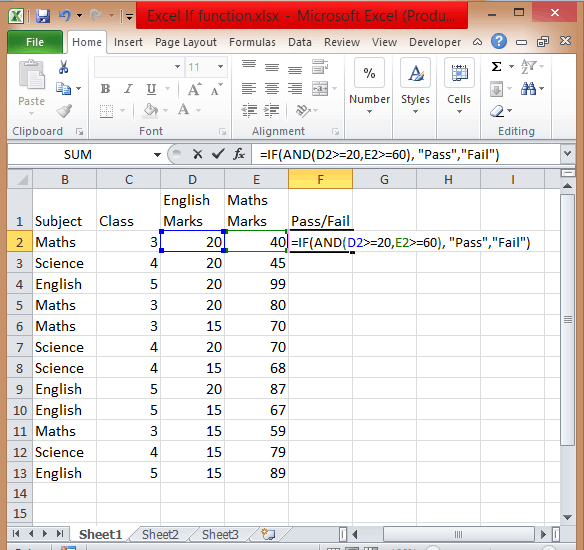
• Apply If & And formula, you will get =IF(AND(D2>=20,E2>=60),”Pass”,”Fail”).

• Add Pass/Fail column in the current table.

• After you have applied this formula, you will find the result in the column.
• Copy the formula from cell F2 and paste in all other cells from F3 to F13.

How to use If with Or function in Excel

To use If and Or statement excel, you need to apply a similar formula as you have applied for If & And with the only difference is that if any of the condition is true then it will show you True.

To apply the formula, you have to follow the above process. The formula is =IF((OR(D2>=20, E2>=60)), “Pass”, “Fail”). If the score is equal or greater than 20 for column D or the second score is equal or greater than 60 then the person is the pass.

How to Use If with And & Or function

If you want to test data based on several multiple conditions then you have to apply both And & Or functions at a single point in time. For example,

Situation 1: If column D>=20 and column E>=60

Situation 2: If column D>=15 and column E>=60

If any of the situations met, then the candidate is passed, else failed. The formula is

=IF(OR(AND(D2>=20, E2>=60), AND(D2>=20, E2>=60)), “Pass”, “Fail”).

4) Excel If Statement with other functions

Above we have learned how to use excel if statement multiple conditions range with And/Or functions. Now we will be going to learn Excel If Statement with other excel functions.

• Excel If with Sum, Average, Min, and Max functions

Let’s take an example where we want to calculate the performance of any student with Poor, Satisfactory, and Good.

If the data set has a predefined structure that will not allow any of the modifications. Then you can add values with this If formula:

=If((A2+B2)>=50, “Good”, If((A2+B2)=>30, “Satisfactory”, “Poor”))

Using the Sum function,

=If(Sum(A2:B2)>=120, “Good”, If(Sum(A2:B2)>=100, “Satisfactory”, “Poor”))

Using the Average function,

=If(Average(A2:B2)>=40, “Good”, If(Average(A2:B2)>=25, “Satisfactory”, “Poor”))

Using Max/Min,

If you want to find out the highest scores, using the Max function. You can also find the lowest scores using the Min function.

=If(C2=Max($C$2:$C$10), “Best result”, “ “)

You can also find the lowest scores using the Min function.

=If(C2=Min($C$2:$C$10), “Worst result”, “ “)

If we combine both these formulas together, then we get

=If(C2=Max($C$2:$C$10), “Best result”, If(C2=Min($C$2:$C$10), “Worst result”, “ “))

You can also call it as nested if functions with other excel functions. To get a result, you can use these if functions with various different functions that are used in excel.

So there are four different ways and types of excel if statements, that you can use according to the situation or condition. Start using it today.

So this is all about Excel If statement multiple conditions ranges, you can also check how to add bullets in excel in our next post.

I hope you found this tutorial useful

You may also like the following Excel tutorials:

• Multiple If Statements in Excel
• Excel Logical test
• How to Compare Two Columns in Excel (using VLOOKUP & IF)
• Using IF Function with Dates in Excel (Easy Examples)

Many people usually asked that how to write an excel nested if statements based on multiple ranges of cells to return different values in a cell? How to nested if statement using date ranges? How to use nested if statement between different values in excel 2013 or 2016?

• Nested IF statements based on multiple ranges
• Nested IF Statement Using Date Ranges
• Nested IF Statements For A Range Of Cells
• Nested IF Statement between different values

This post will guide you how to understand excel nested if statements through some classic examples.

Nested IF statements based on multiple ranges

Assuming that you want to reflect the below request through nested if statements:

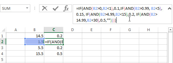
a) If 1<B1<0, Then return 0.1

b) If 0.99<B1<5, then return 0.15

c) If 4.99<B1<15, then return 0.2

d) If 14.99<B1<30, then return 0.5

So if B1 cell was “14.5”, then the formula should be returned “0.2” in the cell.

From above logic request, we can get that it need 4 if statements in the excel formula, and there are multiple ranges so that we can combine with logical function AND in the nested if statements.  The below is the nested if statements that I have tested.

=IF(AND(B1>0,B1<1),0.1,IF(AND(B1>0.99, B1<5),0.15, IF(AND(B1>4.99,B1<15),0.2, IF(AND(B1>14.99,B1<30),0.5,””))))

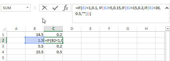
If you don’t want to use AND function in the above nested if statement, can try the below formula:

=IF(B1<1,0.1, If(B1<5,0.15,IF(B1<15,0.2,IF(B1<30,0.5,””))))

Nested IF Statement Using Date Ranges

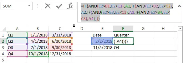
I want to write a nested IF statement to calculated the right Quarter based one the criteria in the below table.

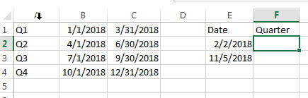
According to the request, we need to compare date ranges, such as: if B1<E2<C1, then return A1.

So we can consider to use AND logical function in the nested if statement. The formula is as follows:

=IF(AND(E2>B1,E2<C1),A1,IF(AND(E2>B2,E2<C2),A2,IF(AND(E2>B3,E2<C3),A3,IF(AND(E2>B4,E2<C3),A4))))

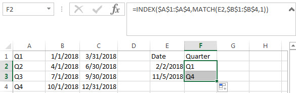
Or we can use INDEX function and combine with MATCH Function to get the right quarter.

=INDEX($A$1:$A$4,MATCH(E2,$B$1:$B$4,1))

Nested IF Statements For A Range Of Cells

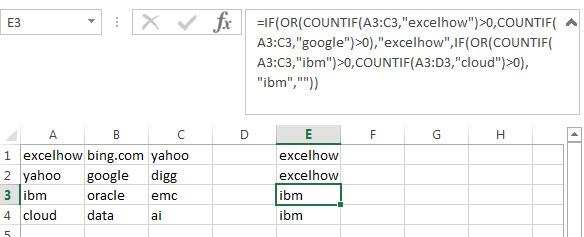
If you have the following requirement and need to write a nested IF statement in excel:

If any of the cells A1 to C1 contain “excelhow”, then return “excelhow” in the cell E1.

If any of the cells A1 to C1 contain “google”, then return “excelhow” in the cell E1.

If any of the cells A1 to C1 contain “ibm”, then return “ibm” in the cell E1.

If any of the cells A1 to C1 contain “Cloud”, then return “ibm” in the cell E1.

How to check if cell ranges A1:C1 contain another string, using “COUNTIF” function is a good choice.

Countif function: Counts the number of cells within a range that meet the given criteria

Let’s try to test the below nested if statement:

=IF(OR(COUNTIF(A3:C3,"excelhow")>0,COUNTIF(A3:C3,"google")>0),"excelhow",IF(OR(COUNTIF(A3:C3,"ibm")>0,COUNTIF(A3:D3,"cloud")>0),"ibm",""))

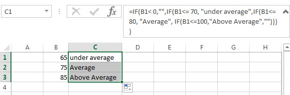
Nested IF Statement between different values

Assuming you have the following different range values, if the B1 has the value 65, then expected to return “under average”in cell C1, if the Cell B1 has the value 75, then return “average” in cell C1. And if the Cell B1 has the value 85, then return “above average” in the cell C1.

0-70	under average
71-80	average
81-100	above average

How do I format the nested if statement in Cell C1 to display the right value? Just try to use the below nested if function or using INDEX function.

=IF(B1< 0,"",IF(B1<= 70, "under average",IF(B1<=80, "Average", IF(B1<=100,"Above Average",""))))

---

• Excel IF function
  The Excel IF function perform a logical test to return one value if the condition is TRUE and return another value if the condition is FALSE. The IF function is a build-in function in Microsoft Excel and it is categorized as a Logical Function.The syntax of the IF function is as below:= IF (condition, [true_value], [false_value])….
• Excel nested if function
  The nested IF function is formed by multiple if statements within one Excel if function. This excel nested if statement makes it possible for a single formula to take multiple actions…
• Excel AND function
  The Excel AND function returns TRUE if all of arguments are TRUE, and it returns FALSE if any of arguments are FALSE.The syntax of the AND function is as below:= AND (condition1,[condition2],…) …
• Excel COUNTIF function
  The Excel COUNTIF function will count the number of cells in a range that meet a given criteria.This function can be used to count the different kinds of cells with number, date, text values, blank, non-blanks, or containing specific characters.etc.The syntax of the COUNTIF function is as below:= COUNTIF (range, criteria) …
• Excel INDEX function
  The Excel INDEX function returns a value from a table based on the index (row number and column number)The INDEX function is a build-in function in Microsoft Excel and it is categorized as a Lookup and Reference Function.The syntax of the INDEX function is as below:= INDEX (array, row_num,[column_num])…
• Excel MATCH  function
  The Excel MATCH function search a value in an array and returns the position of that item.The MATCH function is a build-in function in Microsoft Excel and it is categorized as a Lookup and Reference Function.The syntax of the MATCH function is as below:= MATCH  (lookup_value, lookup_array, [match_type])….

In this example, the goal is to use a formula to check if a specific value exists in a range. The easiest way to do this is to use the COUNTIF function to count occurences of a value in a range, then use the count to create a final result.

COUNTIF function

The COUNTIF function counts cells that meet supplied criteria. The generic syntax looks like this:

=COUNTIF(range,criteria)

Range is the range of cells to test, and criteria is a condition that should be tested. COUNTIF returns the number of cells in range that meet the condition defined by criteria. If no cells meet criteria, COUNTIF returns zero. In the example shown, we can use COUNTIF to count the values we are looking for like this

COUNTIF(data,E5)

Once the named range data (B5:B16) and cell E5 have been evaluated, we have:

=COUNTIF(data,E5)
=COUNTIF(B5:B16,"Blue")
=1

COUNTIF returns 1 because «Blue» occurs in the range B5:B16 once. Next, we use the greater than operator (>) to run a simple test to force a TRUE or FALSE result:

=COUNTIF(data,B5)>0 // returns TRUE or FALSE

By itself, the formula above will return TRUE or FALSE. The last part of the problem is to return a «Yes» or «No» result. To handle this, we nest the formula above into the IF function like this:

=IF(COUNTIF(data,E5)>0,"Yes","No")

This is the formula shown in the worksheet above. As the formula is copied down, COUNTIF returns a count of the value in column E. If the count is greater than zero, the IF function returns «Yes». If the count is zero, IF returns «No».

Slightly abbreviated

It is possible to shorten this formula slightly and get the same result like this:

=IF(COUNTIF(data,E5),"Yes","No")

Here, we have remove the «>0» test. Instead, we simply return the count to IF as the logical_test. This works because Excel will treat any non-zero number as TRUE when the number is evaluated as a Boolean.

Testing for a partial match

To test a range to see if it contains a substring (a partial match), you can add a wildcard to the formula. For example, if you have a value to look for in cell C1, and you want to check the range A1:A100 for partial matches, you can configure COUNTIF to look for the value in C1 anywhere in a cell by concatenating asterisks on both sides:

=COUNTIF(A1:A100,"*"&C1&"*")>0

The asterisk (*) is a wildcard for one or more characters. By concatenating asterisks before and after the value in C1, the formula will count the text in C1 anywhere it appears in each cell of the range. To return «Yes» or «No», nest the formula inside the IF function as above.

An alternative formula using MATCH

As an alternative, you can use a formula that uses the MATCH function with the ISNUMBER function instead of COUNTIF:

=ISNUMBER(MATCH(value,range,0))

The MATCH function returns the position of a match (as a number) if found, and #N/A if not found. By wrapping MATCH inside ISNUMBER, the final result will be TRUE when MATCH finds a match and FALSE when MATCH returns #N/A.

When you need to perform simple arithmetic calculations on several ranges of cells, sum the results, and use criteria to determine which cells to include in the calculations, consider using the SUMPRODUCT function.

SUMPRODUCT takes arrays and arithmetic operators as arguments. You can use arrays that evaluate as True or False (1 or 0) as criteria by using them as factors (multiplying them by the other arrays).

For example, suppose you want to calculate net sales for a particular sales agent by subtracting expenses from gross sales, as in this example.

1. Click a cell outside the ranges you are evaluating. This is where your result goes.

2. Type =SUMPRODUCT(.

3. Type (, enter or select a range of cells to include in your calculations, then type ). For example, to include the column Sales from the table Table1, type (Table1[Sales]).

4. Enter an arithmetic operator: *, /, +, —. This is the operation you will perform using the cells that meet any criteria you include; you can include more operators and ranges. Multiplication is the default operation.

5. Repeat steps 3 and 4 to enter additional ranges and operators for your calculations. After you add the last range you want to include in calculations, add a set of parentheses enclosing all the involved ranges, so that the entire calculation is enclosed. For example, ((Table1[Sales])+(Table1[Expenses])).

   You may need to include additional parentheses inside your calculation to group various elements, depending on the arithmetic you want to perform.

6. To enter a range to use as a criterion, type *, enter the range reference normally, then after the range reference but before the right parenthesis, type =», then the value to match, then «. For example, *(Table1[Agent]=»Jones»). This causes the cells to evaluate as 1 or 0, so when multiplied by other values in the formula the result is either the same value or zero — effectively including or excluding the corresponding cells in any calculations.

7. If you have more criteria, repeat step 6 as needed. After your last range, type ).

   Your completed formula might look like the one in our example above: =SUMPRODUCT(((Table1[Sales])-(Table1[Expenses]))*(Table1[Agent]=B8)), where cell B8 holds the agent name.