If with nested and in excel

The IF function allows you to make a logical comparison between a value and what you expect by testing for a condition and returning a result if that condition is True or False.

=IF(Something is True, then do something, otherwise do something else)

But what if you need to test multiple conditions, where let’s say all conditions need to be True or False (AND), or only one condition needs to be True or False (OR), or if you want to check if a condition does NOT meet your criteria? All 3 functions can be used on their own, but it’s much more common to see them paired with IF functions.

Use the IF function along with AND, OR and NOT to perform multiple evaluations if conditions are True or False.

Syntax

IF(AND()) — IF(AND(logical1, [logical2], …), value_if_true, [value_if_false]))
IF(OR()) — IF(OR(logical1, [logical2], …), value_if_true, [value_if_false]))
IF(NOT()) — IF(NOT(logical1), value_if_true, [value_if_false]))


Argument name	Description
logical_test (required)	The condition you want to test.
value_if_true (required)	The value that you want returned if the result of logical_test is TRUE.

value_if_false (optional)	The value that you want returned if the result of logical_test is FALSE.

Here are overviews of how to structure AND, OR and NOT functions individually. When you combine each one of them with an IF statement, they read like this:

AND – =IF(AND(Something is True, Something else is True), Value if True, Value if False)
OR – =IF(OR(Something is True, Something else is True), Value if True, Value if False)
NOT – =IF(NOT(Something is True), Value if True, Value if False)

Examples

Following are examples of some common nested IF(AND()), IF(OR()) and IF(NOT()) statements. The AND and OR functions can support up to 255 individual conditions, but it’s not good practice to use more than a few because complex, nested formulas can get very difficult to build, test and maintain. The NOT function only takes one condition.

Here are the formulas spelled out according to their logic:

Formula	Description
=IF(AND(A2>0,B2<100),TRUE, FALSE)	IF A2 (25) is greater than 0, AND B2 (75) is less than 100, then return TRUE, otherwise return FALSE. In this case both conditions are true, so TRUE is returned.
=IF(AND(A3=»Red»,B3=»Green»),TRUE,FALSE)	If A3 (“Blue”) = “Red”, AND B3 (“Green”) equals “Green” then return TRUE, otherwise return FALSE. In this case only the first condition is true, so FALSE is returned.
=IF(OR(A4>0,B4<50),TRUE, FALSE)	IF A4 (25) is greater than 0, OR B4 (75) is less than 50, then return TRUE, otherwise return FALSE. In this case, only the first condition is TRUE, but since OR only requires one argument to be true the formula returns TRUE.
=IF(OR(A5=»Red»,B5=»Green»),TRUE,FALSE)	IF A5 (“Blue”) equals “Red”, OR B5 (“Green”) equals “Green” then return TRUE, otherwise return FALSE. In this case, the second argument is True, so the formula returns TRUE.
=IF(NOT(A6>50),TRUE,FALSE)	IF A6 (25) is NOT greater than 50, then return TRUE, otherwise return FALSE. In this case 25 is not greater than 50, so the formula returns TRUE.
=IF(NOT(A7=»Red»),TRUE,FALSE)	IF A7 (“Blue”) is NOT equal to “Red”, then return TRUE, otherwise return FALSE.

Note that all of the examples have a closing parenthesis after their respective conditions are entered. The remaining True/False arguments are then left as part of the outer IF statement. You can also substitute Text or Numeric values for the TRUE/FALSE values to be returned in the examples.

Here are some examples of using AND, OR and NOT to evaluate dates.

Here are the formulas spelled out according to their logic:

Formula	Description
=IF(A2>B2,TRUE,FALSE)	IF A2 is greater than B2, return TRUE, otherwise return FALSE. 03/12/14 is greater than 01/01/14, so the formula returns TRUE.
=IF(AND(A3>B2,A3<C2),TRUE,FALSE)	IF A3 is greater than B2 AND A3 is less than C2, return TRUE, otherwise return FALSE. In this case both arguments are true, so the formula returns TRUE.
=IF(OR(A4>B2,A4<B2+60),TRUE,FALSE)	IF A4 is greater than B2 OR A4 is less than B2 + 60, return TRUE, otherwise return FALSE. In this case the first argument is true, but the second is false. Since OR only needs one of the arguments to be true, the formula returns TRUE. If you use the Evaluate Formula Wizard from the Formula tab you’ll see how Excel evaluates the formula.
=IF(NOT(A5>B2),TRUE,FALSE)	IF A5 is not greater than B2, then return TRUE, otherwise return FALSE. In this case, A5 is greater than B2, so the formula returns FALSE.

Using AND, OR and NOT with Conditional Formatting

You can also use AND, OR and NOT to set Conditional Formatting criteria with the formula option. When you do this you can omit the IF function and use AND, OR and NOT on their own.

From the Home tab, click Conditional Formatting > New Rule. Next, select the “Use a formula to determine which cells to format” option, enter your formula and apply the format of your choice.

Using the earlier Dates example, here is what the formulas would be.

Formula	Description
=A2>B2	If A2 is greater than B2, format the cell, otherwise do nothing.
=AND(A3>B2,A3<C2)	If A3 is greater than B2 AND A3 is less than C2, format the cell, otherwise do nothing.
=OR(A4>B2,A4<B2+60)	If A4 is greater than B2 OR A4 is less than B2 plus 60 (days), then format the cell, otherwise do nothing.
=NOT(A5>B2)	If A5 is NOT greater than B2, format the cell, otherwise do nothing. In this case A5 is greater than B2, so the result will return FALSE. If you were to change the formula to =NOT(B2>A5) it would return TRUE and the cell would be formatted.

Note: A common error is to enter your formula into Conditional Formatting without the equals sign (=). If you do this you’ll see that the Conditional Formatting dialog will add the equals sign and quotes to the formula — =»OR(A4>B2,A4<B2+60)», so you’ll need to remove the quotes before the formula will respond properly.

Need more help?

Introducing IF Function in Excel

Let’s get started with this easy guide to using the IF function and all its related functions in Microsoft Excel, step-by-step with supporting images and examples.

1. IF Function

To learn to use the IF function, we will take an example of a mark list of students below.

Our goal is to find out which student has passed or failed and what are their grades. Of course, it would be a tedious task to find out pass or fail results and grades for each student in this list.

To ease our task, we have IF functions for that matter. The IF function will automatically identify if a student has passed or failed based on the criteria you provide to it.

It will automatically mark a student as “Pass” if he/she has scored above the minimum pass mark and mark a student as “Fail” if he/she has scored below the minimum pass mark.

The IF function automatically assigns the appropriate grades to students based on their marks if you command it.

Here is a glimpse of how the IF function helps you out with assigning grades and marking “Pass” or “Fail”.

Steps to use IF function in Excel

We have allotted certain grades and marked them as Pass or Fail to students based on the percentages they have secured in their exams, with the help of the IF function.

1. Using the IF function in Excel to identify passed/failed students

Let’s learn how we can use the IF formula to achieve this. We will use the same example. We take the minimum passing percentage as 34%.

Find out the percentage of total marks of every student.
Create a new column named “Pass/Fail”.
In the blank cell below the title, type the IF formula as follows next.
Type =IF( and select the first student’s percentage and type >=34.
Put a comma and move to the next argument named [value_if_true]. This means you’re being asked to put a value to be displayed if the above condition is true. Remember these arguments are case sensitive.
Once you have put a comma, type “Pass”.
Put a comma and move to the next argument named [value_if_false] to display a value when the above condition is false. This field is optional in most cases but we need a false value because it is a mark list.
Close the bracket and hit ENTER.

You can see that the formula is displaying “Pass” for the first student because she has secured above 34%.

Double-click or drag the cell from the right corner below to autofill the formula to all the students below.

Recommended read: How to Autofill in Excel?

2. Nested IF Function

Now, let us start assigning grades to all students.

We are going to be using multiple IF functions in a single syntax this time to provide multiple criteria to the IF function. This is called Nested IF in Excel.

However, there is no specific function named “Nested IF” in Excel, it is simply that this behavior has been given a name i.e., Nested IF.

Before we proceed further, we need to first make a table that displays a grading class for each grade. Here is an example below.

Create a new column named “Grade”.
Type the IF function in a blank cell below the title as follows.
Type =IF( and now type AE118>=85,”A”,IF(AE118>=70,”B”,IF(AE118>=55,”C”,IF(AE118>=34,”D”,IF(AE118<=33,”Fail”.

Note that AE118 is our cell address for the first student’s percentage. It will be different in your case. Refer to the image above to make sense of the formula.
The formula simply states- if percentage marks are above and equal to 85 then give “A”, if percentage marks are above and equal to 70 then give “B”, and so on and so forth. For the last condition, we have applied the condition- if the marks are less than or equal to 33 then give “Fail”.
For the last IF statement, you can either put the result as “Fail” or “E” as you like.
Now, note that we will close the formula with 5 brackets for this example as we have used a total of 5 IF formulas.

Hit ENTER to complete the formula.

You can now see that the formula has been applied to the first entry and the result is B because the student has secured 72.5% which is less than 75%. This means the nested Ifs are working correctly.

Now drag the cell from the lower right corner to autofill the formula to the rest of the entries.

You can see that we now have grades and pass/fail markings for every student on the list successfully.

3. IF with AND in Excel

Let us learn the IF formula with the AND function in a single syntax with a minor example.

When you have two or more distinct conditions to be used together, you can use the IF function with AND in Excel.

While nested IFs will also work, using AND function will save your time as it is shorter to type. So, let’s get started.

Our goal is to identify currencies with revenues greater than 20,000 and less than 50,000 and mark them as “Good”.

Type =IF(AND( because we are using the IF with AND function.
Select the first cell under Revenue, and type >20000.
Put a comma and select the first cell under Revenue again and type <50000.
Now, close the bracket to complete the AND function. We’re still working on the IF function so do not put two brackets.
We come back to the IF function as soon as we close the AND function. Now put the values to be displayed if the condition is true or false.
Put a comma to move to the argument [value_if_true] and type “Good”.
You can provide a result in the [value_if_false] argument, but it is completely optional. If nothing is provided then the cells will display FALSE if the condition is false. But if you want the cells to remain blank simply put “” (two double quotation marks) in this argument.
Close the bracket to complete the IF function as well.

This is how the syntax should look like before pressing ENTER.

Hit ENTER to view results and drag the cell down to autofill the formula to the rest of the cells.

There are only two such cells for which the condition is true and the result is being displayed as “Good” for them and the rest of the cells are blank. This means the formula is working correctly.

4. IF with OR in Excel

Using the OR function with the IF function will give results for either of the conditions that are true.

Type =IF(OR(.
Select the first cell under Revenue and type >=20000.
Put a comma and select the first cell under Revenue again and type <=50000.
Now, close the bracket to complete the OR function. We’re still working on the IF function so do not put two brackets.
Coming back to the IF function, we now put the values to be displayed if the condition is true or false.
Put a comma to move to the argument [value_if_true] and type “Flag”.
Put a comma to move to the argument [value_if_false] and type “”.

This is how the syntax should look like before pressing ENTER.

Close the bracket to complete the OR function and hit ENTER.
Drag the cell below to get the results for the rest.

The formula is true for all entries and so it is displaying “Flag” for all of them. This is because all the values are either lower than 50,000 or greater than 20,000.

Conclusion

This was all about IF functions and other related functions to the IF function that are AND and OR functions.

Reference: ExcelJet

Источник

This formula relies on a technique called «nested IFs» to handle a series of options and results. With nested IFs, one IF function is nested inside another, a process that is explained in some detail here.

The formula in this example is purposely more verbose that necessary in order to «show» all possible options and results in a way that is easier to understand and maintain. The trick is to structure the formula with line breaks to show each IF on a separate line along with the «true result» for that IF. The «false result» is the following IF statement. Notice the final false result will «catch» any case that fails all previous tests.

Essentially, we are using line breaks to build a «table»that the human eye can easily read. To limit IF functions, we are using the AND function to run more than one logical test at a time. The AND function inside each IF function tests both color and value.

Note can use use Alt + Enter to enter to enter new lines in the formula bar. You’ll need to expand the formula bar vertically in order to see more than one line at a time.

More conditions

This formula approach can be expanded to evaluate more options. The AND function can handle more logical tests, and you can combine the AND function with the OR function if needed. You could also replace AND and OR with boolean logic. Finally, you can also use the IFS function in later versions of Excel to reduce nesting.

Result as calculation

Although the example above shows a numeric result for each set of options, the formula can be customized to run a calculation instead by replacing hardcoded values with any standard formula expression.

Источник

Things will not always be the way we want them to be. The unexpected can happen. For example, let’s say you have to divide numbers. Trying to divide any number by zero (0) gives an error. Logical functions come in handy such cases. In this tutorial, we are going to cover the following topics.

In this tutorial, we are going to cover the following topics.

What is a Logical Function?
IF function example
Excel Logic functions explained
Nested IF functions

What is a Logical Function?

It is a feature that allows us to introduce decision-making when executing formulas and functions. Functions are used to;

Check if a condition is true or false
Combine multiple conditions together

What is a condition and why does it matter?

A condition is an expression that either evaluates to true or false. The expression could be a function that determines if the value entered in a cell is of numeric or text data type, if a value is greater than, equal to or less than a specified value, etc.

IF Function example

We will work with the home supplies budget from this tutorial. We will use the IF function to determine if an item is expensive or not. We will assume that items with a value greater than 6,000 are expensive. Those that are less than 6,000 are less expensive. The following image shows us the dataset that we will work with.

Put the cursor focus in cell F4
Enter the following formula that uses the IF function

=IF(E4<6000,”Yes”,”No”)

HERE,

“=IF(…)” calls the IF functions
“E4<6000” is the condition that the IF function evaluates. It checks the value of cell address E4 (subtotal) is less than 6,000
“Yes” this is the value that the function will display if the value of E4 is less than 6,000
“No” this is the value that the function will display if the value of E4 is greater than 6,000

When you are done press the enter key

You will get the following results

Excel Logic functions explained

The following table shows all of the logical functions in Excel

S/N	FUNCTION	CATEGORY	DESCRIPTION	USAGE
01	AND	Logical	Checks multiple conditions and returns true if they all the conditions evaluate to true.	=AND(1 > 0,ISNUMBER(1)) The above function returns TRUE because both Condition is True.
02	FALSE	Logical	Returns the logical value FALSE. It is used to compare the results of a condition or function that either returns true or false	FALSE()
03	IF	Logical	Verifies whether a condition is met or not. If the condition is met, it returns true. If the condition is not met, it returns false. =IF(logical_test,[value_if_true],[value_if_false])	=IF(ISNUMBER(22),”Yes”, “No”) 22 is Number so that it return Yes.
04	IFERROR	Logical	Returns the expression value if no error occurs. If an error occurs, it returns the error value	=IFERROR(5/0,”Divide by zero error”)
05	IFNA	Logical	Returns value if #N/A error does not occur. If #N/A error occurs, it returns NA value. #N/A error means a value if not available to a formula or function.	=IFNA(D6*E6,0) N.B the above formula returns zero if both or either D6 or E6 is/are empty
06	NOT	Logical	Returns true if the condition is false and returns false if condition is true	=NOT(ISTEXT(0)) N.B. the above function returns true. This is because ISTEXT(0) returns false and NOT function converts false to TRUE
07	OR	Logical	Used when evaluating multiple conditions. Returns true if any or all of the conditions are true. Returns false if all of the conditions are false	=OR(D8=”admin”,E8=”cashier”) N.B. the above function returns true if either or both D8 and E8 admin or cashier
08	TRUE	Logical	Returns the logical value TRUE. It is used to compare the results of a condition or function that either returns true or false	TRUE()

A nested IF function is an IF function within another IF function. Nested if statements come in handy when we have to work with more than two conditions. Let’s say we want to develop a simple program that checks the day of the week. If the day is Saturday we want to display “party well”, if it’s Sunday we want to display “time to rest”, and if it’s any day from Monday to Friday we want to display, remember to complete your to do list.

A nested if function can help us to implement the above example. The following flowchart shows how the nested IF function will be implemented.

The formula for the above flowchart is as follows

=IF(B1=”Sunday”,”time to rest”,IF(B1=”Saturday”,”party well”,”to do list”))

HERE,

“=IF(….)” is the main if function
“=IF(…,IF(….))” the second IF function is the nested one. It provides further evaluation if the main IF function returned false.

Practical example

Create a new workbook and enter the data as shown below

Enter the following formula

=IF(B1=”Sunday”,”time to rest”,IF(B1=”Saturday”,”party well”,”to do list”))

Enter Saturday in cell address B1
You will get the following results

Download the Excel file used in Tutorial

Summary

Logical functions are used to introduce decision-making when evaluating formulas and functions in Excel.

Источник

The AND Function in excel is a logical function that tests multiple conditions and returns “true” or “false” depending on whether they are met or not. The formula of AND function is “=AND(logical1,[logical2]…),” where “logical1” is the first condition to evaluate.

You are free to use this image on your website, templates, etc, Please provide us with an attribution linkArticle Link to be Hyperlinked
For eg:
Source: AND Function in Excel (wallstreetmojo.com)

AND Function in Excel
- Syntax of the AND Function
- The Characteristics of AND Function
- The Output of AND Function
- How to Use AND Function in Excel?
  - Example #1–AND Function
  - Example #2–AND Function With Nested IF Function
  - Example #3–AND Function With Nested IF Function
- Nesting of AND Function in Excel
  - Example #4–Nested AND Function
- Limitations of AND Function
- Frequently Asked Questions
- Recommended Articles

Syntax of the AND Function

The syntax is stated as follows:

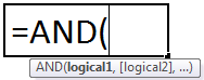
The function accepts the following arguments:

Logical 1: This is the first condition or logical value to evaluate.
Logical 2: This is the second condition or logical value to evaluate.

The “logical 1” is a mandatory argument and “logical 2” is an optional argument.

The Characteristics of AND Function

It returns “true” if all conditions or logical values evaluate to true.
It returns “false” if any of the conditions or logical values evaluates to false.
It can have more logical values depending on the situation and the requirement.
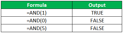
It treats the value zero as “false” and all non-zero values as “true” while evaluating numbers.
It ignores empty cells provided as an argument.
It is often used in combination with other Excel functionsExcel functions help the users to save time and maintain extensive worksheets. There are 100+ excel functions categorized as financial, logical, text, date and time, Lookup & Reference, Math, Statistical and Information functions.read more like IF, OR, and so on.

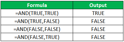
The Output of AND Function

The output in different situations is given as follows:

The output while evaluating numbers is given as follows:

How to Use AND Function in Excel?

It is easy to use the AND function. Let us understand its working with the help of a few examples.

You can download this AND Function Excel Template here – AND Function Excel Template

Example #1–AND Function

There are three levels and ten players in a game. To be a winner, a player has to clear all three levels. The player loses if he/she fails in any of the three levels.

The performance of the players in different levels is given in the following table. We are required to determine the winner.

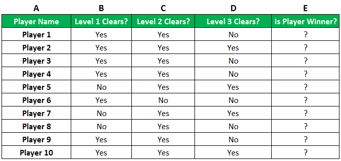
We apply AND formula in column E.

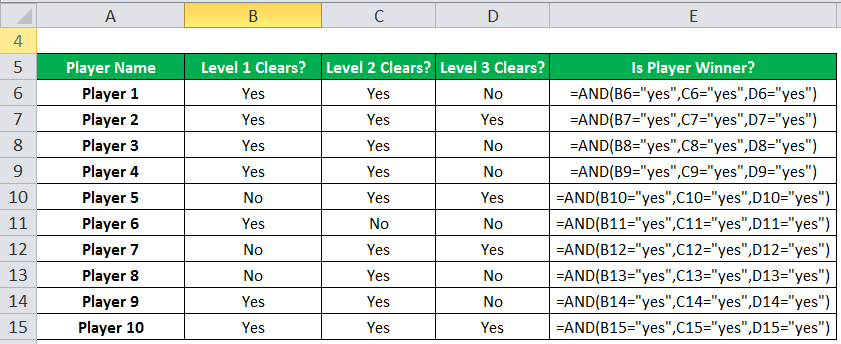
The output of the formula appears in column E.

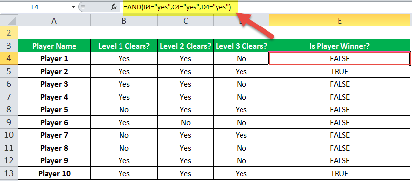
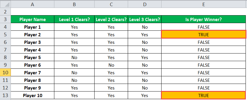
Player 2 and player 10 have cleared all the levels. Since all the logical conditions for these two players are met, the AND function gives the output “true.”

The rest of the players were unable to clear all three levels. If any of the levels is not cleared, the AND function returns “false.”

Example #2–AND Function With Nested IF Function

Let us consider the following example.

We have the marks (in percentage) of ten students in a school. We have to determine the grade obtained by each student according to the criteria given.

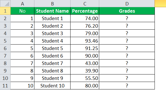
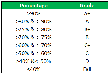
A student obtains “A+” if he/she scores more than 90%. If the percentage is greater than or equal to 80% but less than or equal to 90%, grade “A” is given.

If the percentage is less than 40%, the student fails. Likewise, the grades for the different percentages are given in the following table.

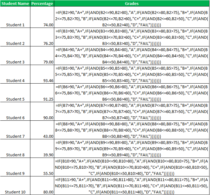
We apply the following formula.

“=IF(B2>90,”A+”,IF(AND(B2<=90,B2>80),”A”,IF(AND(B2<=80,B2>75),”B+”,IF(AND(B2<=75,B2>70),”B”,IF(AND(B2<=70,B2>60),”C+”,IF(AND(B2<=60,B2>50),”C”,IF(AND(B2<=50,B2>40),”D”,”FAIL”)))))))”

We use the nested IF functionIn Excel, nested if function means using another logical or conditional function with the if function to test multiple conditions. For example, if there are two conditions to be tested, we can use the logical functions AND or OR depending on the situation, or we can use the other conditional functions to test even more ifs inside a single if.read more with multiple AND functions to compute the grades. The latter allows testing two conditions together.

The syntax of the IF function is stated as follows:

“=IF(logical_test,[value_if_true],[value_if_false])”

The IF function returns “true” if the condition is met, else returns “false.”

The first logical test is “B2>90.” If this condition is “true,” grade “A+” is assigned. If this condition is “false,” the IF function evaluates the next condition.

The next logical testA logical test in Excel results in an analytical output, either true or false. The equals to operator, “=,” is the most commonly used logical test.read more is “B2<=90, B2>80.” If this condition is “true,” grade “A” is assigned. If this condition is “false,” the next statement is evaluated. Likewise, the IF function tests every condition given in the formula.

The last logical test is “B2<=50, B2>40.” If this condition is “true,” grade “D” is assigned, else the student fails.

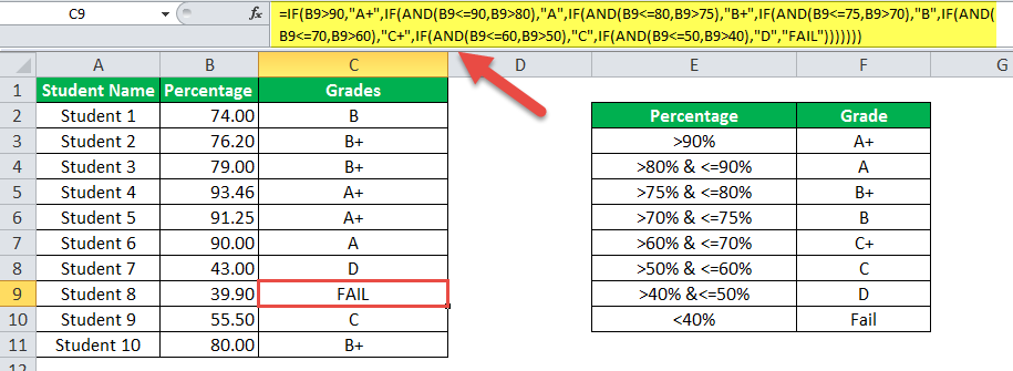
We apply the formula to all categories of students, as shown in the following image.

The output of the formula is shown in the succeeding image.

Example #3–AND Function With Nested IF Function

The name of employees and the sales revenueSales revenue refers to the income generated by any business entity by selling its goods or providing its services during the normal course of its operations. It is reported annually, quarterly or monthly as the case may be in the business entity’s income statement/profit & loss account.read more generated by them for an organization are shown in the succeeding image. Every employee is given a monetary incentive depending on the total sales made by him/her.

We have to calculate the incentives of all the employees based on their performance.

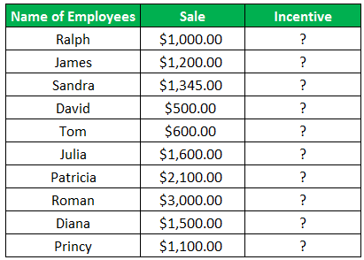
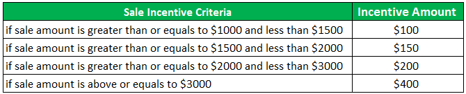
The incentive criteria followed by the organization is given in the succeeding table.

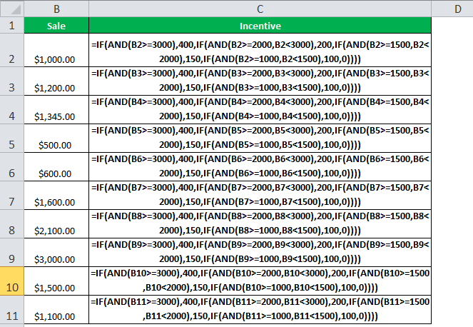
We apply the following formula.

“=IF(AND(B2>=3000),400,IF(AND(B2>=2000,B2<3000),200,IF(AND(B2>=1500,B2<2000),150,IF(AND(B2>=1000,B2<1500),100,0))))”

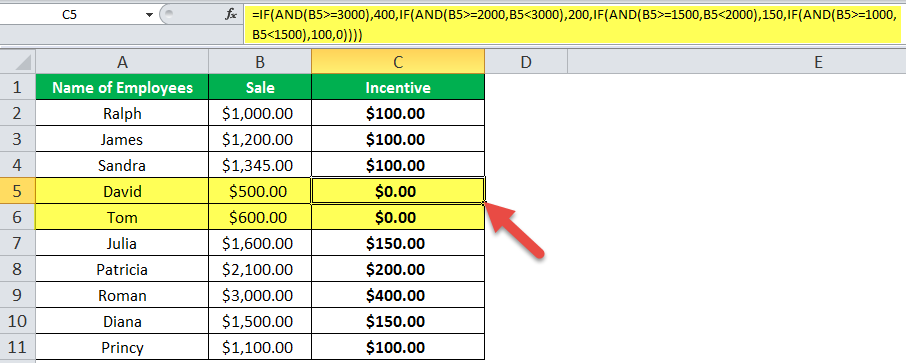
We use multiple IFs In Excel, multiple IF conditions are IF statements that are contained within another IF statement. They are used to test multiple conditions at the same time and return distinct values. Additional IF statements can be included in the ‘value if true’ and ‘value if false’ arguments of a standard IF formula.read moreand multiple AND functions to calculate the incentives received by all the employees, as shown in the following table.

Roman generates sales revenue of $3000. So, he receives an incentive amount of $400.

The revenue generated by David and Tom is $500 and $600, respectively. To be eligible for an incentive, minimum sales of $1000 is required. Hence, they do not get any incentive.

Nesting of AND Function in Excel

A nested function refers to using a function inside another Excel function. In Excel, the nesting of functions up to 64 levels is allowed.

Example #4–Nested AND Function

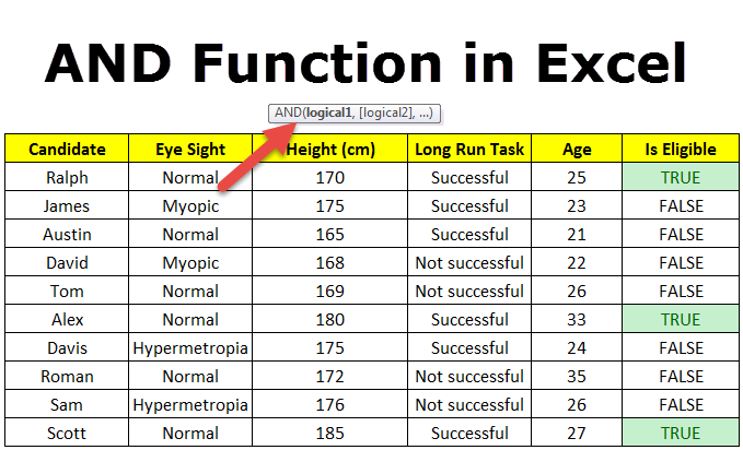
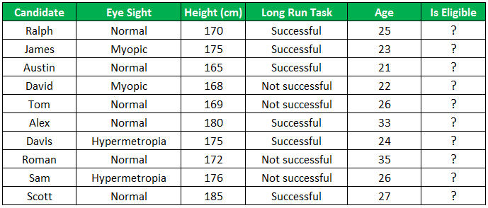
We have a list of candidates who wish to join the Army subject to certain conditions. The eligibility criteria are stated as follows:

The age should be greater than or equal to 18, but less than 35 years.
The height should be greater than 167 cm.
The eyesight should be normal.
The candidate must have completed the long-run task.

We need to find out the candidates who are eligible for joining the Army.

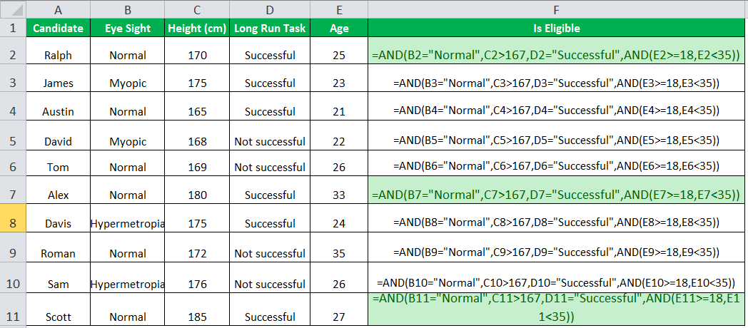
To evaluate the candidates on the given parameters, we use the nested AND function.

We apply the following formula.

“=AND(B2=”Normal”,C2>167,D2=”Successful”,AND(E2>=18,E2<35))”

We evaluate multiple logical conditions simultaneously. We also check whether the age is within the prescribed limit or not. So, we use the AND function inside another AND function.

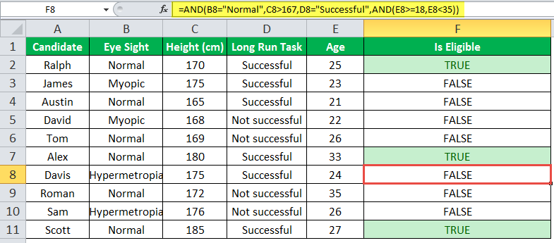
The output of the formula is shown in the succeeding image.

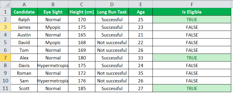
The candidates Ralph, Alex, and Scott pass the selection criteria. Hence, their eligibility output (in column F) is “true.” The remaining candidates are not eligible for joining the Army.

Limitations of AND Function

The limitations are listed as follows:

With Excel 2007 onwards, the AND function can test up to 255 arguments given that the length of the formula does not exceed 8,162 characters.
In Excel 2003 and previous versions, the AND function can test up to 30 arguments given that the length of the formula does not exceed 1,024 characters.
The AND function returns “#VALUE! error#VALUE! Error in Excel represents that the reference cell the user has either entered an incorrect formula or used a wrong data type (mostly numerical data). Sometimes, it is difficult to identify the kind of mistake behind this error.read more” if logical conditions are passed as text or if none of the arguments evaluates to a logical value.
The AND function returns “#VALUE! error” if all the arguments provided are empty cells.

The following two images show the output of the AND function when an empty cell and a text string is provided as an argument.

Frequently Asked Questions

#1 – When should the AND function of Excel be used

#2 – How is the AND function used with the OR function in Excel?

The OR function helps compare two values or statements. The AND function is combined with the OR function by the following formulas:

“=AND(OR(Condition1,Condition2),Condition3)”
“=AND(OR(Condition1,Condition2),OR(Condition3,Condition4)”
“=OR(AND(Condition1,Condition2),Condition3)”
“=OR(AND(Condition1,Condition2),AND(Condition3,Condition4))”

#3 – What is the difference between AND, IF, and OR functions in Excel?

The difference between the three functions is stated as follows:

– The AND function helps evaluate multiple conditions at the same time. It returns “true” when all conditions are true; otherwise, it returns “false.”
– The IF function helps compare the value with the result expected by the user. It returns specific values for the “true” and “false” outcomes.
– The OR function helps compare two values or two statements. It returns “true” when at least one of the specified conditions is met. It returns “false” if all the logical values evaluate to false.

The AND function tests multiple conditions and returns “true” or “false” depending upon whether they are met or not.
The AND function returns “true” if all conditions evaluate to true and returns “false” if any of the conditions evaluates to false.
The AND function treats the value zero as “false.”
The AND function can test up to 255 arguments in the latest versions of Excel.
The AND function returns “#VALUE! error” if logical conditions are passed as a text.
The formula of the IF function is “=IF(logical_test,[value_if_true],[value_if_false]).”

Examples

Using AND, OR and NOT with Conditional Formatting

Need more help?

See also

Introducing IF Function in Excel

1. IF Function

Steps to use IF function in Excel

1. Using the IF function in Excel to identify passed/failed students

2. Nested IF Function

3. IF with AND in Excel

4. IF with OR in Excel

Conclusion

More conditions

Result as calculation

What is a Logical Function?

IF Function example

Excel Logic functions explained

Practical example

Summary

Table of contents

Syntax of the AND Function

The Characteristics of AND Function

The Output of AND Function

How to Use AND Function in Excel?

Example #1–AND Function

Example #2–AND Function With Nested IF Function

Example #3–AND Function With Nested IF Function

Nesting of AND Function in Excel

Example #4–Nested AND Function

Limitations of AND Function

Frequently Asked Questions

Recommended Articles