
IF function
The IF function is one of the most popular functions in Excel, and it allows you to make logical comparisons between a value and what you expect.
So an IF statement can have two results. The first result is if your comparison is True, the second if your comparison is False.
For example, =IF(C2=”Yes”,1,2) says IF(C2 = Yes, then return a 1, otherwise return a 2).

Use the IF function, one of the logical functions, to return one value if a condition is true and another value if it’s false.
IF(logical_test, value_if_true, [value_if_false])
For example:
-
=IF(A2>B2,»Over Budget»,»OK»)
-
=IF(A2=B2,B4-A4,»»)
|
Argument name |
Description |
|---|---|
|
logical_test (required) |
The condition you want to test. |
|
value_if_true (required) |
The value that you want returned if the result of logical_test is TRUE. |
|
value_if_false (optional) |
The value that you want returned if the result of logical_test is FALSE. |
Simple IF examples

-
=IF(C2=”Yes”,1,2)
In the above example, cell D2 says: IF(C2 = Yes, then return a 1, otherwise return a 2)

-
=IF(C2=1,”Yes”,”No”)
In this example, the formula in cell D2 says: IF(C2 = 1, then return Yes, otherwise return No)As you see, the IF function can be used to evaluate both text and values. It can also be used to evaluate errors. You are not limited to only checking if one thing is equal to another and returning a single result, you can also use mathematical operators and perform additional calculations depending on your criteria. You can also nest multiple IF functions together in order to perform multiple comparisons.

-
=IF(C2>B2,”Over Budget”,”Within Budget”)
In the above example, the IF function in D2 is saying IF(C2 Is Greater Than B2, then return “Over Budget”, otherwise return “Within Budget”)

-
=IF(C2>B2,C2-B2,0)
In the above illustration, instead of returning a text result, we are going to return a mathematical calculation. So the formula in E2 is saying IF(Actual is Greater than Budgeted, then Subtract the Budgeted amount from the Actual amount, otherwise return nothing).

-
=IF(E7=”Yes”,F5*0.0825,0)
In this example, the formula in F7 is saying IF(E7 = “Yes”, then calculate the Total Amount in F5 * 8.25%, otherwise no Sales Tax is due so return 0)
Note: If you are going to use text in formulas, you need to wrap the text in quotes (e.g. “Text”). The only exception to that is using TRUE or FALSE, which Excel automatically understands.
Common problems
|
Problem |
What went wrong |
|---|---|
|
0 (zero) in cell |
There was no argument for either value_if_true or value_if_False arguments. To see the right value returned, add argument text to the two arguments, or add TRUE or FALSE to the argument. |
|
#NAME? in cell |
This usually means that the formula is misspelled. |
Need more help?
You can always ask an expert in the Excel Tech Community or get support in the Answers community.

See Also
IF function — nested formulas and avoiding pitfalls
IFS function
Using IF with AND, OR and NOT functions
COUNTIF function
How to avoid broken formulas
Overview of formulas in Excel
Need more help?
Want more options?
Explore subscription benefits, browse training courses, learn how to secure your device, and more.
Communities help you ask and answer questions, give feedback, and hear from experts with rich knowledge.
What to Know
- The syntax of IF-THEN is =IF(logic test,value if true,value if false).
- The first argument tells the function what to do if the comparison is true.
- The second argument tells the function what to do if the comparison is false.
This article explains how to use the IF-THEN function in Excel for Microsoft 365, Excel 2019, 2016, 2013, 2010; Excel for Mac, and Excel Online, as well as a few examples.
Inputting IF-THEN in Excel
The IF-THEN function in Excel is a powerful way to add decision making to your spreadsheets. It tests a condition to see if it’s true or false and then carries out a specific set of instructions based on the results.
For example, by inputting an IF-THEN in Excel, you can test if a specific cell is greater than 900. If it is, you can make the formula return the text «PERFECT.» If it isn’t, you can make the formula return «TOO SMALL.»
There are many conditions you can enter into the IF-THEN formula.
The IF-THEN function’s syntax includes the name of the function and the function arguments inside of the parenthesis.
This is the proper syntax of the IF-THEN function:
=IF(logic test,value if true,value if false)
The IF part of the function is the logic test. This is where you use comparison operators to compare two values.
The THEN part of the function comes after the first comma and includes two arguments separated by a comma.
- The first argument tells the function what to do if the comparison is true.
- The second argument tells the function what to do if the comparison is false.
A Simple IF-THEN Function Example
Before moving on to more complex calculations, let’s look at a straightforward example of an IF-THEN statement.
Our spreadsheet is set up with cell B2 as $100. We can input the following formula into C2 to indicate whether the value is larger than $1000.
=IF(B2>1000,"PERFECT","TOO SMALL")
This function has the following arguments:
- B2>1000 tests whether the value in cell B2 is larger than 1000.
- «PERFECT» returns the word PERFECT in cell C2 if B2 is larger than 1000.
- «TOO SMALL» returns the phrase TOO SMALL in cell C2 if B2 is not larger than 1000.
The comparison part of the function can compare only two values. Either of those two values can be:
- Fixed number
- A string of characters (text value)
- Date or time
- Functions that return any of the values above
- A reference to any other cell in the spreadsheet containing any of the above values
The TRUE or FALSE part of the function can also return any of the above. This means that you can make the IF-THEN function very advanced by embedding additional calculations or functions inside of it (see below).
When inputting true or false conditions of an IF-THEN statement in Excel, you need to use quotation marks around any text you want to return, unless you’re using TRUE and FALSE, which Excel automatically recognizes. Other values and formulas don’t require quotation marks.
Inputting Calculations Into the IF-THEN Function
You can embed different calculations for the IF-THEN function to perform, depending on the comparison results.
In this example, one calculation is used to calculate the tax owed, depending on the total income in B2.
The logic test compares total income in B2 to see if it’s greater than $50,000.00.
=IF(B2>50000,B2*0.15,B2*0.10)
In this example, B2 is not larger than 50,000, so the «value_if_false» condition will calculate and return that result.
In this case, that’s B2*0.10, which is 4000.
The result is placed into cell C2, where the IF-THEN function is inserted, will be 4000.
You can also embed calculations into the comparison side of the function.
For example, if you want to estimate that taxable income will only be 80% of total income, you could change the above IF-THEN function to the following.
=IF(B2*0.8>50000,B2*0.15,B2*0.10)
This will perform the calculation on B2 before comparing it to 50,000.
Never enter a comma when entering numbers in the thousands. This is because Excel interprets a comma as the end of an argument inside of a function.
Nesting Functions Inside of an IF-THEN Function
You can also embed (or «nest») a function inside of an IF-THEN function.
This lets you perform advanced calculations and then compare the actual results to the expected results.
In this example, let’s say you have a spreadsheet with five students’ grades in column B. You could average those grades using the AVERAGE function. Depending on the class average results, you could have cell C2 return either «Excellent!» or «Needs Work.»
This is how you would input that IF-THEN function:
=IF(AVERAGE(B2:B6)>85,"Excellent!","Needs Work")
This function returns the text «Excellent!» in cell C2 if the class average is over 85. Otherwise, it returns «Needs Work.»
As you can see, inputting the IF-THEN function in Excel with embedded calculations or functions allows you to create dynamic and highly functional spreadsheets.
FAQ
-
How do I create multiple IF-THEN statements in Excel?
-
How many IF statements can you nest in Excel?
You can nest up to 7 IF statements within a single IF-THEN statement.
-
How does conditional formatting work in Excel?
With conditional formatting in Excel, you can apply more than one rule to the same data to test for different conditions. Excel first determines if the various rules conflict, and, if so, the program determines which conditional formatting rule to apply to the data.
Thanks for letting us know!
Get the Latest Tech News Delivered Every Day
Subscribe
The IF function is useful for making quick decisions or performing comparisons in Microsoft Excel. It’s an easy but versatile logical comparison function for handling many scenarios, ranging from financial models to assigning allowances. In this tutorial, I’ll show how to use the IF function in Excel and a simple adaptation. (Includes practice worksheet)
What is the IF Function?
The IF function is one of the simplest and most useful logical functions. It can fill cell items for you based on evaluating a condition such as a cell’s content and logical operators. What’s appealing about the function is that it can be used with other functions to handle more complex scenarios. You might think of it as a formula building block and you can find it in the Logical category.
The wizard-like dialog allows you to fill 3 Function Arguments or data elements, but you could use the formula bar once you master it. This is the easiest way to learn an Excel formula because you can see if it returns your expected result. For example, at the bottom left of the dialog, a line reads “Formula result =.”
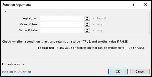
The IF Function Arguments
| Field | Definition |
|---|---|
| Logical_test | A test on a cell value that is either TRUE or FALSE. |
| Value_if_true | The value Excel will put in a cell if the test is true. |
| Value_if_false | The value Excel will put in a cell if the test fails. |
Despite not having Microsoft Excel, my parents routinely employed this type of IF logic when calculating my allowance. Their version read:
IF you empty the garbage AND mow the lawn AND wash the dishes AND walk the dog, you get your full allowance.
And since I grew up in New England, this logic would change with the seasons to account for leaves and snow.
Setting Up the IF Function
Although Excel can’t issue an allowance, it can calculate the amount using a logic test based on whether a cell met a formula condition.
For example, I could create a spreadsheet with the chores needed to get an allowance. If the chores were completed (TRUE situation), a value would be applied toward the allowance. If the chore wasn’t completed (FALSE situation), nothing would be added.
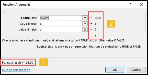
These examples are noted by labels [1] and [2] in the screen snap below.

Using the example above, you might express the logic in the following way:
IF cell B2 equals “Y”, then use the Rate value from cell C2 ($3.00) in D2.
IF cell B2 does not equal “Y”, then place 0 in cell D2.
As you can see in this example, the IF logical condition is either TRUE or FALSE. And it pays to take out the garbage.
Comparison Operators
To help evaluate conditions, Excel uses a list of common operators. You probably know these as we probably used them in math class. These operators will be evaluated to a logical “true” or “false”. In the table below, B2 and C2 in the Example column are cell references.
| Operator | Example |
| = (equals) | B2 = “YES” |
| < (less than) | B2 < 12 |
| > (greater than) | B2 > 112 |
| <= (less than or equal to) | B2 <= 12 |
| >= (greater than or equal to) | B2 >= 12 |
| <> (not equal to) | B2 <> C2 |
How To Enter IF Function Arguments
- Click the spreadsheet cell where you wish to use the Excel formula.
- From the Formulas tab, click Insert function…
- In the Insert Function dialog text box, type “if“.
Note: On Office 365, there is now a Logical button on the Formulas tab. You can select IF from the drop-down menu.
- Make sure your cursor is in the Logical_test text box.
- Click the spreadsheet cell you wish to evaluate. Excel will fill in the cell reference such as “B2”.
- Add the equals sign = and your desired value in quotes. For example =”Y”.
- In the Value_if_true field, type the value you would like entered in your cell if B2 equals “Y”. In our example, I’ll click cell C3.
- In the Value_if_false: field, enter the value the cell should have if B2 does not have a “Y”. I’ll enter 0. I could leave it blank, but the cell would show “FALSE”.
- Review the dialog to see if the Formula result= value (label [1] below) is what you expect. If not, check to see if any errors show to the right of the fields (label [2] below).
- Click OK.
- Copy the formula to the other cells in your column.
✪ Tip: Even though the Value_if_false field is optional, it’s best to provide a value. Otherwise, Excel will use FALSE in the cell value.
Excel IF With Numeric Values
The above spreadsheet might have been Version 1 for my parents. A new incentive program would appear based on some parent/child negotiations and competitive neighborhood rates. I probably would’ve requested pay for partial chores. No doubt, my parents would counter with a penalty clause if something was less than half done.
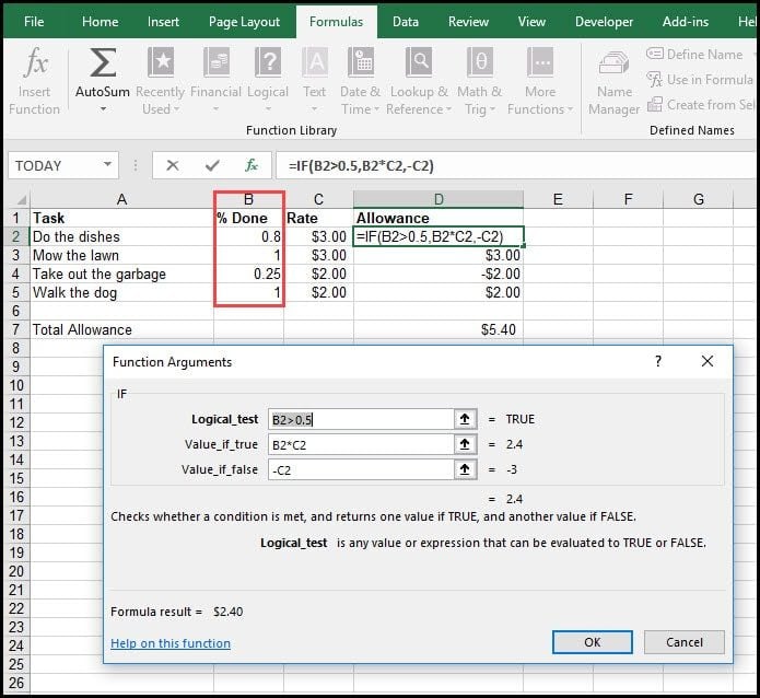
Excel is flexible when it comes to IF statements and can evaluate more than a simple “Y” or “N.” For example, if we convert our previous Done? column to a % Done column with a number, we can accommodate these new requirements such as:
=IF(B2>0.5,B2*C2,-C2)The new formula returns the allowance based on the % Done in Column B. If the chore completion number is greater than .5, a prorated amount is applied to the allowance.
If the chore completion rate was .5 or below, a negative amount was applied to the allowance. Loosely translated, an “incomplete” performance costs money. You could also apply colors using conditional formatting.
Troubleshooting Tips
There are a couple of reasons why the IF function doesn’t work as expected.
- You don’t have quotes around a text string. For example, you used B2=Y instead of B2=”Y”. The quotes aren’t needed if you use the values TRUE or FALSE as Excel recognizes them.
- You have a data type mismatch. For example, your comparison operator was comparing a number in one cell such as “twelve”, but the comparison cell had 12. However, Excel is forgiving if you’re evaluating number formats such as 1.5 versus $1.50.
As you’ve seen, this is a versatile and useful function. Once you get the hang of how to use IF function in Excel, you’ll start using it in more scenarios. The two examples presented here were foundational. But you can use IF functions to handle other transactions such as applying sales tax, stock values, shipping charges, fixing Excel DIV 0 errors, or even nesting IF functions with Boolean logic.
And if you have kids, let them build the Excel spreadsheet and give them a bonus for using the IF function.
Hand-picked Excel Tutorials
- How to Use Excel VLOOKUP
- Beginner’s Guide to XLOOKUP
- How to Create an Excel Pivot Table
- The Benefits of Creating Excel Tables
- Video: How to Use Conditional Formatting
What is IF Function in Excel?
IF function in Excel evaluates whether a given condition is met and returns a value depending on whether the result is “true” or “false”. It is a conditional function of Excel, which returns the result based on the fulfillment or non-fulfillment of the given criteria.
For example, the IF formula in Excel can be applied as follows:
“=IF(condition A,“value B”,“value C”)”
The IF excel function returns “value B” if condition A is met and returns “value C” if condition A is not met.
It is often used to make logical interpretations which help in decision-making.
Table of contents
- What is IF Function in Excel?
- Syntax of the IF Excel Function
- How to Use IF Function in Excel?
- Example #1
- Example #2
- Example #3
- Example #4
- Example #5
- Guidelines for the Multiple IF Statements
- Frequently Asked Question
- IF Excel Function Video
- Recommended Articles
Syntax of the IF Excel Function
The syntax of the IF function is shown in the following image:

The IF excel function accepts the following arguments:
- Logical_test: It refers to the condition to be evaluated. The condition can be a value or a logical expression.
- Value_if_true: It is the value returned as a result when the condition is “true”.
- Value_if_false: It is the value returned as a result when the condition is “false”.
In the formula, the “logical_test” is a required argument, whereas the “value_if_true” and “value_if_false” are optional arguments.
The IF formula uses logical operators to evaluate the values in a range of cells. The following table shows the different logical operatorsLogical operators in excel are also known as the comparison operators and they are used to compare two or more values, the return output given by these operators are either true or false, we get true value when the conditions match the criteria and false as a result when the conditions do not match the criteria.read more and their meaning.
| Operator | Meaning |
|---|---|
| = | Equal to |
| > | Greater than |
| >= | Greater than or equal to |
| < | Less than |
| <= | Less than or equal to |
| <> | Not equal to |
How to Use IF Function in Excel?
Let us understand the working of the IF function with the help of the following examples in Excel.
You can download this IF Function Excel Template here – IF Function Excel Template
Example #1
If there is no oxygen on a planet, life is impossible. If oxygen is available on a planet, then life is possible. The following table shows a list of planets in column A and the information on the availability of oxygen in column B. We have to find the planets where life is possible, based on the condition of oxygen availability.

Let us apply the IF formula to cell C2 to find out whether life is possible on the planets listed in the table.
The IF formula is stated as follows:
“=IF(B2=“Yes”, “Life is Possible”, “Life is Not Possible”)
The succeeding image shows the IF formula applied to cell C2.

The subsequent image shows how the IF formula is applied to the range of cells C2:C5.

Drag the cells to view the output of all the planets.

The output in the below worksheet shows life is possible on the planet Earth.
Flow Chart of Generic IF Excel Function

The IF Function Flow Chart for Mars (Example #1)

The flow of IF function flowchart for Jupiter and Venus is the same as the IF function flowchart for Mars (Example #1).
The IF Function Flow Chart for Earth

Hence, the IF excel function allows making logical comparisons between values. The modus operandi of the IF function is stated as: If something is true, then do something; otherwise, do something else.
Example #2
The following table shows a list of years. We want to find out if the given year is a leap year or not.
A leap year has 366 days; the extra day is the 29th of February. The criteria for a leap year are stated as follows:
- The year will be exactly divisible by 4 and not exactly be divisible by 100 or
- The year will be exactly divisible by 400.

In this example, we will use the IF function along with the AND, OR, and MOD functions to find the leap years.
We use the MOD function to find a remainder after a dividend is divided by a divisor.
The AND functionThe AND function in Excel is classified as a logical function; it returns TRUE if the specified conditions are met, otherwise it returns FALSE.read more evaluates both the conditions of the leap years for the value “true”. The OR functionThe OR function in Excel is used to test various conditions, allowing you to compare two values or statements in Excel. If at least one of the arguments or conditions evaluates to TRUE, it will return TRUE. Similarly, if all of the arguments or conditions are FALSE, it will return FASLE.read more evaluates either of the condition for the value “true”.
We will apply the MOD function to the conditions as follows:
If MOD(year,4)=0 and MOD(year,100)<>(is not equal to) 0, then the year is a leap year.
or
If MOD(year,400)=0, then the year is a leap year; otherwise, the year is not a leap year.
The IF formula is stated as follows:
“=IF(OR(AND((MOD(year,4)=0),(MOD(year,100)<>0)),(MOD(year,400)=0)),“Leap Year”, “Not A Leap Year”)”
The argument “year” refers to a reference value.
The following images show the output of the IF formula applied in the range of cells.


The following image shows how the IF formula is applied to the range of cells B2:B18.

The succeeding table shows the years 1960, 2028, and 2148 as leap years and the remaining as non-leap years.

The result of the IF excel formula is displayed for the range of cells B2:B18 in the following image.

Example #3
The succeeding table shows a list of drivers and the directions they undertook to reach the destination. It is preceded by an image of the road intersection explaining the turns taken by the drivers and their destinations. The right turn leads to town B, and the left turn leads to town C. Identify the driver’s destination to town B and town C.
Road Intersection Image


Let us apply the IF excel function to find the destination. Here, the condition is mentioned as follows:
- If the driver turns right, he/she reaches town B.
- If the driver turns left, he/she reaches town C.
We use the following IF formula to find the destination:
“=IF(B2=“Left”, “Town C”, “Town B”)”
The succeeding image shows the output of the IF formula applied to cell C2.

Drag the cells to use the formula in the range C2:C11. Finally, we get the destinations of each driver for their turning movements.
The below image displays the IF formula applied to the range.

The output of the IF formula and the destinations are displayed in the succeeding image.

The result shows that six drivers reached town C, and the remaining four have reached town B.
Example #4
The following table shows a list of items and their inventory levels. We want to check if the specific item is available in the inventory or not using the IF function.

Let us list the name of items in column A and the number of items in column B. The list of data to be validated for the entire items list is shown in the cell E2 of the below image.

We use the Excel IF along with the VLOOKUP functionThe VLOOKUP excel function searches for a particular value and returns a corresponding match based on a unique identifier. A unique identifier is uniquely associated with all the records of the database. For instance, employee ID, student roll number, customer contact number, seller email address, etc., are unique identifiers.
read more to check the availability of the items in the inventory.
The VLOOKUP function looks up the values referring to the number of items, and the IF function will check whether the item number is greater than zero or not.
We will apply the following IF formula in the F2 cell:
“=IF(VLOOKUP(E2,A2:B11,2,0)=0, “Item Not Available”,“Item Available”)”
If the lookup value of an item is equal to 0, then the item is not available; else, the item is available.
The succeeding image shows the result of the IF formula in the cell F2.

Select “bat” in the E2 item cell to know whether the item is available or not in the inventory (as shown in the following image).

Example #5
The following table shows the list of students and their marks. The grade criteria are provided based on the marks obtained by the students. We want to find the grade of each student in the list.

We apply the Nested IF in Excel since we have multiple criteria to find and decide each student’s grade.
The Nesting of IF function uses the IF function inside another IF formula when multiple conditions are to be fulfilled.
The syntax of Nesting of IF function is stated as follows:
“=IF( condition1, value_if_true1, IF( condition2, value_if_true2, value_if_false2 ))”
The succeeding table represents the range of scores and the grades, respectively.

Let us apply the multiple IF conditions with AND function in the below-nested formula to find out the grade of the students:
“=IF((B2>=95),“A”,IF(AND(B2>=85,B2<=94),“B”,IF(AND(B2>=75,B2<=84),“C”,IF(AND(B2>=61,B2<=74),“D”,“F”))))”
The IF function checks the logical condition as shown in the formula below:
“=IF(logical_test, [value_if_true],[value_if_false])”
We will split the above-mentioned nested formula and check the IF statements as shown below:
First Logical Test: B2>=95
If the formula returns,
- Value_if_true, execute: “A” (Grade A) else(comma) enter value_if_false
- Value_if_false, then the formula finds another IF condition and enter IF condition
Second Logical Test: B2>=85(logical expression 1) and B2<=94(logical expression 2)
(We use AND function to check the multiple logical expressions as the two given conditions are to be evaluated for “true.”)
If the formula returns,
- Value_if_true, execute: “B” (Grade B) else(comma) enter value_if_false
- Value_if_false, then the formula finds another IF condition and enter IF condition
Third Logical Test: B2>=75(logical expression 1) and B2<=84(logical expression 2)
(We use AND function to check the multiple logical expressions as the two given conditions are to be evaluated for “true.”)
If the formula returns,
- Value_if_true, execute: “C” (Grade C) else(comma) enter value_if_false
- value_if_false, then the formula finds another IF condition and enter IF condition
Fourth Logical Test: B2>=61(logical expression 1) and B2<=74(logical expression 2)
(We use AND function to check the multiple logical expressions as the two given conditions are to be evaluated for “true.”)
If the formula returns,
- Value_if_true, execute: “D” (Grade D) else(comma) enter value_if_false
- Value_if_false, execute: “F” (Grade F)
- Finally, close the parenthesis.
The below image displays the output of the IF formula applied to the range.

The succeeding image shows the IF nested formula applied to the range.

The grades of the students are listed in the following table.

Guidelines for the Multiple IF Statements
The guidelines for the multiple IF statements are listed as follows:
- Use nested IF function to a limited extent as multiple IF statements require a great deal of thought to be accurate.
- Multiple IF statementsIn Excel, multiple IF conditions are IF statements that are contained within another IF statement. They are used to test multiple conditions at the same time and return distinct values. Additional IF statements can be included in the ‘value if true’ and ‘value if false’ arguments of a standard IF formula.read more require multiple parentheses (), which is often difficult to manage. Excel provides a way to check the color of each opening and closing parenthesis to avoid this situation. The last closing parenthesis color will always be black, denoting the end of the formula statement.
- Whenever we pass a string value for the arguments “value_if_true” and “value_if_false” or test a reference against a string value, enclose the string value in double quotes. Passing a string value without quotes will result in “#NAME?” error.
Frequently Asked Question
1. What is the IF function in Excel?
The Excel IF function is a logical function that checks the given criteria and returns one value for a “true” and another value for a “false” result.
The syntax of the IF function is stated as follows:
“=IF(logical_test, [value_if_true], [value_if_false])”
The arguments are as follows:
1. Logical_test – It refers to a value or condition that is tested.
2. Value_if_true – It is the value returned when the condition logical_test is “true.”
3. Value_if_false – It is the value returned when the condition logical_test is “false.”
The “logical_test” is a required argument, whereas the “value_if_true” and “value_if_false” are optional arguments.
2. How to use the IF Excel function with multiple conditions?
The IF Excel statement for multiple conditions is created by using multiple IF functions in a single formula.
The syntax of IF function with multiple conditions is stated as follows:
“=IF (condition 1_“true”, do something, IF (condition 2_“true”, do something, IF (condition 3_ “true”, do something, else do something)))”
3. How to use the function IFERROR in Excel?
IF Excel Function Video
Recommended Articles
This has been a guide to the IF function in Excel. Here we discuss how to use the IF function along with examples and downloadable templates. You may also look at these useful functions –
- What is the Logical Test in Excel?A logical test in Excel results in an analytical output, either true or false. The equals to operator, “=,” is the most commonly used logical test.read more
- “Not Equal to” in Excel“Not Equal to” argument in excel is inserted with the expression <>. The two brackets posing away from each other command excel of the “Not Equal to” argument, and the user then makes excel checks if two values are not equal to each other.read more
- Data Validation ExcelThe data validation in excel helps control the kind of input entered by a user in the worksheet.read more
The logical IF statement in Excel is used for the recording of certain conditions. It compares the number and / or text, function, etc. of the formula when the values correspond to the set parameters, and then there is one record, when do not respond — another.
Logic functions — it is a very simple and effective tool that is often used in practice. Let us consider it in details by examples.
The syntax of the function «IF» with one condition
The operation syntax in Excel is the structure of the functions necessary for its operation data.
=IF(boolean;value_if_TRUE;value_if_FALSE)
Let us consider the function syntax:
- Boolean – what the operator checks (text or numeric data cell).
- Value_if_TRUE – what will appear in the cell when the text or numbers correspond to a predetermined condition (true).
- Value_if_FALSE – what appears in the box when the text or the number does not meet the predetermined condition (false).
Example:

Logical IF functions.
The operator checks the A1 cell and compares it to 20. This is a «Boolean». When the contents of the column is more than 20, there is a true legend «greater 20». In the other case it’s «less or equal 20».
Attention! The words in the formula need to be quoted. For Excel to understand that you want to display text values.
Here is one more example. To gain admission to the exam, a group of students must successfully pass a test. The results are listed in a table with columns: a list of students, a credit, an exam.

The statement IF should check not the digital data type but the text. Therefore, we prescribed in the formula В2= «done» We take the quotes for the program to recognize the text correctly.
The function IF in Excel with multiple conditions
Usually one condition for the logic function is not enough. If you need to consider several options for decision-making, spread operators’ IF into each other. Thus, we get several functions IF in Excel.
The syntax is as follows:
Here the operator checks the two parameters. If the first condition is true, the formula returns the first argument is the truth. False — the operator checks the second condition.
Examples of a few conditions of the function IF in Excel:

It’s a table for the analysis of the progress. The student received 5 points:
- А – excellent;
- В – above average or superior work;
- C – satisfactory;
- D – a passing grade;
- E – completely unsatisfactory.
IF statement checks two conditions: the equality of value in the cells.

In this example, we have added a third condition, which implies the presence of another report card and «twos». The principle of the operator is the same.
Enhanced functionality with the help of the operators «AND» and «OR»
When you need to check out a few of the true conditions you use the function И. The point is: IF A = 1 AND A = 2 THEN meaning в ELSE meaning с.
OR function checks the condition 1 or condition 2. As soon as at least one condition is true, the result is true. The point is: IF A = 1 OR A = 2 THEN value B ELSE value C.
Functions AND & OR can check up to 30 conditions.
An example of using the operator AND:

It’s the example of using the logical operator OR.

How to compare data in two tables
Users often need to compare the two spreadsheets in an Excel to match. Examples of the «life»: compare the prices of goods in different bringing, to compare balances (accounting reports) in a few months, the progress of pupils (students) of different classes, in different quarters, etc.
To compare the two tables in Excel, you can use the COUNTIFS statement. Consider the order of application functions.
For example, consider the two tables with the specifications of various food processors. We planned allocation of color differences. This problem in Excel solves the conditional formatting.
Baseline data (tables, which will work with):

Select the first table. Conditional Formatting — create a rule — use a formula to determine the formatted cells:

In the formula bar write: = COUNTIFS (comparable range; first cell of first table)=0. Comparing range is in the second table.
To drive the formula into the range, just select it first cell and the last. «= 0» means the search for the exact command (not approximate) values.
Choose the format and establish what changes in the cell formula in compliance. It’s better to do a color fill.
Select the second table. Conditional Formatting — create a rule — use the formula. Use the same operator (COUNTIFS). For the second table formula:
Download all examples in Excel

Now it is easy to compare the characteristics of the data in the table.