If value is not zero excel

Home / Excel Formulas / IF Negative Then Zero (0) – (Excel Formula)

Let me share an example with you. In the following table, you have a table with the two lists of the number in columns A and B. And in column C, you have a difference between both.

Now here need to use a formula to change negative values into zeros. So in this tutorial, we look at all the different ways to write a formula to convert negative numbers into zeros.

Convert Negative Numbers using IF

The first method is to use the IF function that allows you to create a condition to check if a number is negative and then convert that number into a zero.

Use the following steps.

1. Enter the IF function in cell C2.
2. Specify the subtraction formula for cell A1 from B1.
3. Use the greater sign with the zero to create a condition.
4. For the value_if_true, specify zero.
5. And for the value_if_false, enter the subtraction formula that you have used in the condition.
6. Enter the closing parentheses and hit enter to get the result.

By using the above steps, you have written a formula that subtracts two values and tests the result. If the result is a negative number, then convert that negative number into a zero, or else the normal result.

=IF(A2-B2<0,0,A2-B2)

Change Negative Numbers into a Zero with MAX Function

You can also use the MAX function to change a negative number into a zero. Let’s take the same example.

=MAX(A2-B2,0)

In the above formula, you have used the max function where one argument is the subtraction formula of A2 from B2 and the second one is a zero.

Let’s Understand it this way, the max function returns the maximum values from multiple values. When the result of the subtraction is a positive number it returns that number, but if the result is a negative number, it returns zero.

Show a Zero for a Negative Number

You can also use custom formatting to show a zero for a negative number. Use the below steps to apply it.

1. Select a cell or range of cells.
2. Press the Shortcut key Control + 1 (Command +1 if you are using Mac) to open the Format Cells dialog box.
3. Click on the Custom Option and enter the 0;”0″;0 into the input box.
4. Click OK to apply the settings.

This method won’t change the value but the formatting. The original value will stay intact.

Download Sample File

• Ready

And, if you want to Get Smarter than Your Colleagues check out these FREE COURSES to Learn Excel, Excel Skills, and Excel Tips and Tricks.

If the return cell in an Excel formula is empty, Excel by default returns 0 instead. For example cell A1 is blank and linked to by another cell. But what if you want to show the exact return value – for empty cells as well as 0 as return values? This article introduces three different options for dealing with empty return values.

Option 1: Don’t display zero values

Probably the easiest option is to just not display 0 values. You could differentiate if you want to hide all zeroes from the entire worksheet or just from selected cells.

There are three methods of hiding zero values.

1. Hide zero values with conditional formatting rules.
2. Blind out zeros with a custom number format.
3. Hide zero values within the worksheet settings.

For details about all three methods of just hiding zeroes, please refer to this article.

One small advice on my own account: My Excel add-in “Professor Excel Tools” has a built-in Layout Manager. With this, you can apply this formatting easily to a complete Excel workbook.

Give it a try? Click here and the download starts right away.

Option 2: Change zeroes to blank cells

Unlike the first option, the second option changes the output value. No matter if the return value is 0 (zero) or originally a blank cell, the output of the formula is an empty cell. You can achieve this using the IF formula.

Say, your lookup formula looks like this: =VLOOKUP(A3,C:D,2,FALSE)  (hereafter referred to by “original formula”). You want to prevent getting a zero even if the return value―found by the VLOOKUP formula in column D―is an empty value. This can be achieved using the IF formula.

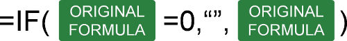
The structure of such IF formula is shown in the image above (if you need assistance with the IF formula, please refer to this article). The original formula is wrapped within the IF formula. The first argument compares if the original formula returns 0. If yes―and that’s the task of the second argument―the formula returns nothing through the double quotation marks. If the orgininal formula within the first argument doesn’t return zero, the last argument returns the real value. This is achieved by the original formula again.

The complete formula looks like this.

=IF(VLOOKUP(A3,C:D,2,FALSE)=0,"",VLOOKUP(A3,C:D,2,FALSE))

Option 3: Show zeroes but don’t show blank or empty return values

The previous option two didn’t differentiate between 0 and empty cells in the return cell. If you only want to show empty cells if the return cell found by your lookup formula is empty (and not if the return value really is 0) then you have to slightly alter the formula from option 2 before.

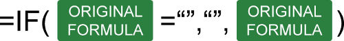
Like before, the IF formula is wrapped around the original formula. But instead of testing if the return value is 0, it tests within the first argument if the return value is blank. This is done by the double quotation marks. The rest of the formula is the as before: With the second argument you define that—if the value from the original formula is blank—the return value is empty too. If not, the last argument defines that you return the desired non-blank value.

The formula in your example from option 2 looks like this.

=IF(VLOOKUP(A3,C:D,2,FALSE)="","",VLOOKUP(A3,C:D,2,FALSE))

Option 4: Use Professor Excel Tools to insert the IF functions very quickly

To save some time, we have included a feature for showing blank cells (instead of zeros) in our Excel add-in Professor Excel Tools.

It’s very simple:

1. Select the cells that are supposed to return blanks (instead of zeros).
2. Click on the arrow under the “Return Blanks” button on the Professor Excel ribbon and then on either
   1. Return blanks for zeros and blanks or
   2. Return zeros for zeros and blanks for blanks.

Professor Excel then inserts the IF function as shown in options 2 and 3 above.

Option 5: One elegant solution for not returning zero values…

… was written in the comments. Thanks, Dom! Great to get such awesome feedback from you!

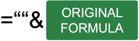
It’s actually quite straight forward: Add two quotation marks in front or after the function and concatenate it with the “&”-character. So, in this case the VLOOKUP function from above would look like this:

=""&VLOOKUP(A3,C:D,2,FALSE)

But: There is a downside. This method forces the cell to a text / string value. This might cause problems in further calculations if a zero is returned. Let me give you an example:

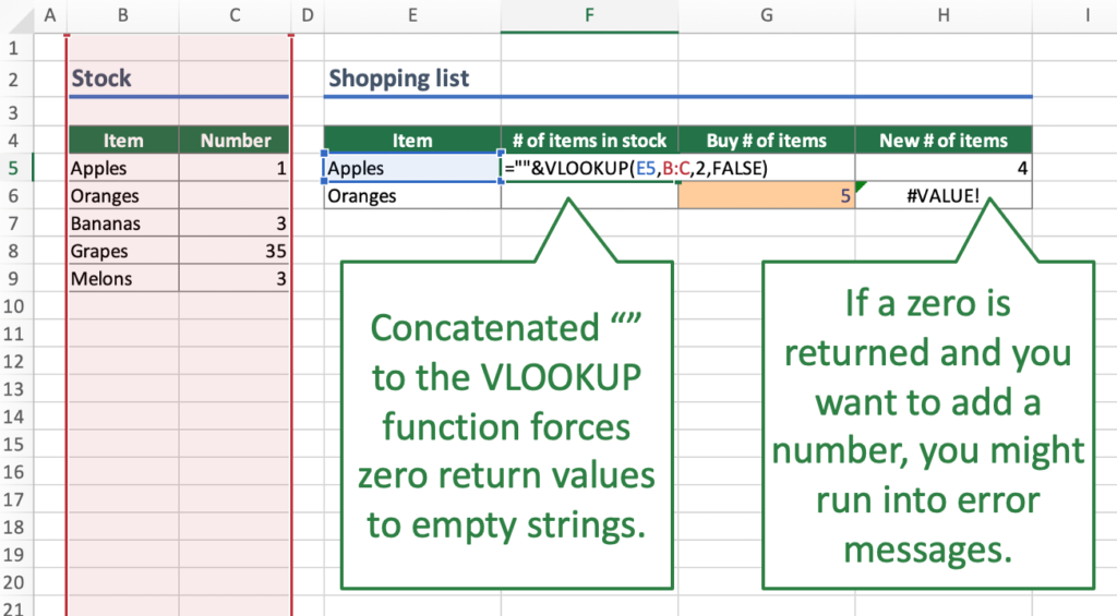
Careful: Return value is interpretated as text.Your VLOOKUP function above is concatenated to an empty string “”. If your return value is 0, the cell will be shown as an empty string. Further calculations might be difficult: For example, if you want to add a number to the return value. Referring directly to the cell, for example =F6+G6 leads to the #VALUE error message as shown above. However, using the SUM function =SUM(F6,G6) still works.

Bottom line: This is an elegant approach, but please test it well if it suits to your Excel model.

Image by Pexels from Pixabay

Sometimes you need to check if a cell is blank, generally because you might not want a formula to display a result without input.

In this case we’re using IF with the ISBLANK function:

• =IF(ISBLANK(D2),»Blank»,»Not Blank»)

Which says IF(D2 is blank, then return «Blank», otherwise return «Not Blank»). You could just as easily use your own formula for the «Not Blank» condition as well. In the next example we’re using «» instead of ISBLANK. The «» essentially means «nothing».

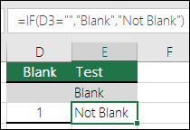
=IF(D3=»»,»Blank»,»Not Blank»)

This formula says IF(D3 is nothing, then return «Blank», otherwise «Not Blank»). Here is an example of a very common method of using «» to prevent a formula from calculating if a dependent cell is blank:

• =IF(D3=»»,»»,YourFormula())

  IF(D3 is nothing, then return nothing, otherwise calculate your formula).

An accrual ledger should note zeroes, even if that is the hyphen displayed with an Accounting style number format. However, if you want to leave the line blank when there are no values to calculate use a formula like the following,

 =IF(COUNT(F16:G16), SUM(G16, INDEX(H$1:H15, MATCH(1e99, H$1:H15)), -F16), "")

That formula is a little tricky because you seem to have provided your sample formula from somewhere down into the entries of the ledger’s item rows without showing any layout or sample data. The formula I provided should be able to be put into H16 and then copied or filled to other locations in column H but I offer no guarantees without seeing the layout.

If you post some sample data or a publicly available link to a screenshot showing your data layout more specific assistance could be offered. http://imgur.com/ is a good place to host a screenshot and it is likely that someone with more reputation will insert the image into your question for you.

Watch Video – How to Hide Zero Values in Excel + How to Remove Zero Values

In case you prefer reading over watching a video, below is the complete written tutorial.

Sometimes in Excel, you may want to hide zero values in your dataset and show these cells as blanks.

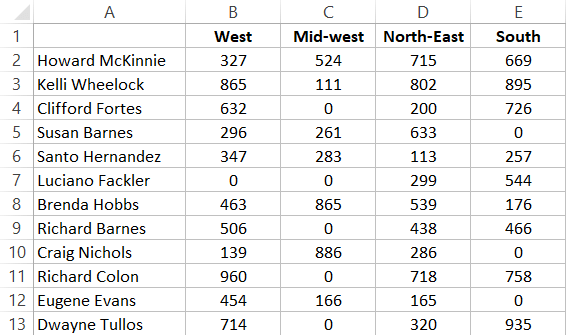
Suppose you have a dataset as shown below and you want to hide the value 0 in all these cells (or want to replace it with something such as a dash or the text ‘Not Available’).

While you can do this manually with a small dataset, you’ll need better ways when working with large datasets.

In this tutorial, I will show you multiple ways to hide zero values in Excel and one method to select and remove all the zero values from the dataset.

Important Note: When you hide a 0 in a cell using the methods shown in this tutorial, it will only hide the 0 and not remove it. While the cells may look empty, those cells still contain the 0s. And in case you use these cells (that have hidden zeroes) in any formula, these will be used in the formula.

Let’s get started and dive into each of these methods!

Automatically Hide Zero Value in Cells

Excel has an inbuilt functionality that allows you to automatically hide all the zero values for the entire worksheet.

All you have to do is uncheck a box in Excel options, and the change will be applied to the entire worksheet.

Suppose you have the sales dataset as shown below and you want to hide all the zero values and show a blank cells instead.

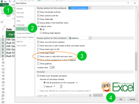
Below are the steps to hide zeros from all the cells in a workbook in Excel:

1. Open the workbook in which you want to hide all the zeros
2. Click the File tab
3. Click on Options
4. In the Excel Options dialog box that opens, click on the ‘Advanced’ option in the left pane
5. Scroll down to the section that says ‘Display option for this worksheet’, and select the worksheet in which you want to hide the zeros.
6. Uncheck the ‘Show a zero in cells that have zero value’ option
7. Click Ok

The above steps would instantly hide zeros in all the cells in the selected worksheet.

This change is also applied to cells where zero is a result of a formula.

Remember that this method only hides the 0 value in the cells and doesn’t remove these. The 0 is still there, it’s just hidden.

This is the best and fastest method to hide zero values in Excel. But this is useful only if you want to hide zero values in the entire worksheet. In case you only want this to hide zero values in a specific range of cells, it’s better to use other methods covered next in this tutorial.

Hide Zero Value in Cells using Conditional Formatting

While the above method is the most convenient one, it doesn’t allow you to hide zeros only in a specific range (rather it hides zero values in the entire worksheet).

In case you only want to hide zeros for a specific dataset (or multiple datasets), you can use conditional formatting.

With conditional formatting, you can apply a specific format based on the value in the cells. So, if the value in some cells is 0, you can simply program conditional formatting to hide it (or even highlight it if you want).

Suppose you have a dataset as shown below and you want to hide zeros in the cells.

Below are the steps to hide zeros in Excel using conditional formatting:

1. Select the dataset
2. Click the ‘Home’ tab
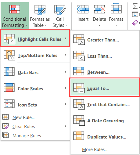
3. In the ‘Styles’ group, click on ‘Conditional Formatting’.
4. Place the cursor over the ‘Highlight Cells Rules’ options and in the options that show up, click on the ‘Equal to’ option.
5. In the ‘Equal To’ dialog box, enter ‘0’ in the left field.
6. Select the Format drop-down and click on ‘Custom Format’.
7. In the ‘Format Cells’ dialog box, select the ‘Font’ tab.
8. From the Color drop-down, choose the white color.
9. Click OK.
10. Click OK.

The above steps change the font color of the cells that have the zeros to white, which make these cells look blank.

This workaround works only when you have a white background in your worksheet. In case there is any other background-color in the cells, the white color may still keep the zeros visible.

In case you want to truly hide the zeros in the cells, where the cells look blank no matter what background color is given to the cells, you can use the steps below.

1. Select the dataset
2. Click the ‘Home’ tab
3. In the ‘Styles’ group, click on ‘Conditional Formatting’.
4. Place the cursor over the ‘Highlight Cells Rules’ options and in the options that show up, click on the ‘Equal to’ option.
5. In the ‘Equal To’ dialog box, enter 0 in the left field.
6. Select the Format drop-down and click on Custom Format.
7. In the ‘Format Cells’ dialog box, select the ‘Number’ tab and click on the ‘Custom’ option in the left pane.
8. In the Custom format option, enter the following in the Type field: ;;; (three semi-colons without space)
9. Click OK.
10. Click OK.

The above steps change the custom formatting of cells that have the value 0.

When you use three semi-colons as the format, it hides everything in the cell (be it numeric or text). And since this format is applied only to those cells which have the value 0 in it, it only hides the zeros and not the rest of the dataset.

You can also use this method to highlight these cells in a different color (such as red or yellow). To do this, just add another step (after Step where you need to select the Fill tab in the ‘Format cells’ dialog box and then select the color in which you want to highlight the cells.

Both the methods covered above also work when 0 is a result of a formula in a cell.

Note: Both the method covered in this section only hide the zero values. It doesn’t remove these zeros. This means that in case you use these cells in calculations, all the zeros will be used as well.

Hide Zero Value using Custom Formatting

Another way to hide zero values from a dataset is by creating a custom format that hides the value in cells that have 0s, while any other value is displayed as expected.

Below are the steps to use a custom format to hide zeros in cells:

1. Select the entire dataset for which you want to apply this format. If you want this for the entire worksheet, select all the cells
2. With the cells selected, click the Home tab
3. In the Cells group, click the Format option
4. From the drop-down option, click on Format Cells. This will open the Format cells dialog box
5. In the Format Cells dialog box, select the Number tab
6. In the option on the left pane, click on the Custom option.
7. In the options on the right, enter the following format in the Type field: 0;-0;;@
8. Click OK

The above steps would apply a custom format to the selected cells where only those cells which have the value 0 are formatted to hide the value, while the rest of the cells display the data as expected.

How does this custom format work?

In Excel, there are four types of data formats that you specify:

1. Positive numbers
2. Negative numbers
3. Zeros
4. Text

And for each of these data types, you can specify a format.

In most cases, there is a default format – General, which keeps all these data types visible. But you have the flexibility of creating a specific format for each of these data types.

Below is the custom format structure you need to follow in case you are applying a custom format to each of these data types:

<Positive Numbers>;<Negative Numbers>;<Zeros>;<Text>

In the method covered above, I have specified the format to:

0;-0;;@

The above format does the following:

1. Positive numbers are shown as is
2. Negative numbers are shown with a negative sign
3. Zeros are hidden (as no format is specified)
4. Text is shown as is

Replace Zeros with Dash or Some Specific Text

In some cases, you may want to not just hide the zeros in the cells, but replace these with something more meaning.

For example, you may want to remove the zeros and replace it with a dash or a text such as “Not Available” or “Data Yet to Come”

This is again made possible using custom number formatting, where you can specify what a cell should display instead of a zero.

Below are the steps to convert a 0 to a dash in Excel:

1. Select the entire dataset for which you want to apply this format. If you want this for the entire worksheet, select all the cells
2. With the cells selected, click the Home tab
3. In the Cells group, click the Format option
4. From the drop-down option, click on Format Cells. This will open the Format cells dialog box
5. In the Format Cells dialog box, select the Number tab
6. In the option on the left pane, click on the Custom option.
7. In the options on the right, enter the following format in the Type field: 0;-0;–;@
8. Click OK

The above steps would keep all the other cells as is and change the cells with the value 0 to show a dash (–).

Note: In this example, I have chosen to replace the zero with a dash, but you can use any text as well. For example, if you want to show the NA in the cells, you can use the following format: 0;-0;”NA”;@

Pro Tip: You can also specify a few text colors in custom number formatting. For example, if you want the cells with zeros to show the text NA in red color, you can use the following format: 0;-0;[Red]”NA”;@

Hide Zero Values in Pivot Tables

There can be two scenarios where a Pivot Table shows the value as 0:

1. The source data cells that are summarized in the Pivot Table has 0 values
2. The source data cells that are summarized in the Pivot Table are blanks and the Pivot table has been formatted to show the empty cells as zero

Let’s see how to hide the zeros in the Pivot table in each scenario:

When Source Data cells have 0s

Below is a sample dataset that I have used to create a Pivot table. Note that the Quantity/Revenue/Profit numbers for all the records for ‘West’ are 0.

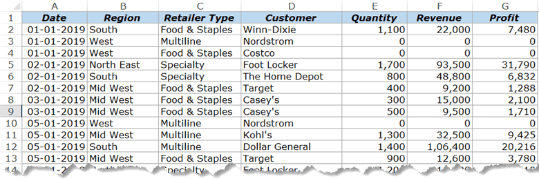
The Pivot table created using this data set looks as shown below:

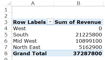
Since there were 0s in the dataset for all the records for West region, you see a 0 in the Pivot table for west here.

If you want to hide zero in this Pivot Table, you can use conditional formatting to do this.

However, conditional formatting in the Pivot Table in Excel works a little different than regular data.

Here are the steps to apply conditional formatting to Pivot Table to hide zeros:

1. Select any cell in the column that has 0s in the Pivot Table summary (Do not select all the cells, but only one cell)
2. Click the Home tab
3. In the ‘Styles’ group, click on ‘Conditional Formatting’.
4. Place the cursor over the ‘Highlight Cells Rules’ options and in the options that show up, click on the ‘Equal to’ option.
5. In the ‘Equal To’ dialog box, enter 0 in the left field.
6. Select the Format drop-down and click on Custom Format.
7. In the ‘Format Cells’ dialog box, select the Number tab and click on the ‘Custom’ option in the left pane.
8. In the Custom format option, enter the following in the Type field: ;;; (three semi-colons without space)
9. Click OK. You will see small Formatting Options icon at the right of the selected cell.
10. Click on this ‘Formatting Options’ icon
11. In the options that become available, choose – All cells showing “Sum of Revenue” values for “Region”.

The above steps hide the zero in the Pivot Table in such a way that if you change the Pivot Table structure (by adding more rows/columns headers to it, the zeros will continue to be hidden).

If you want to learn more about how this works, here is a detailed tutorial on the right way to apply conditional formatting to Pivot Tables.

When Source Data cells have empty cells

Below is an example where I have a dataset that has empty cells for all the records for West.

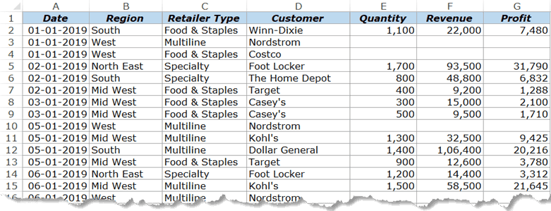
If I create a Pivot Table using this data, I will get the result as shown below.

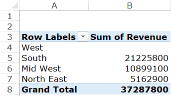
By default, the Pivot Table shows you empty cells when all the cells in the source data are blank. But in case you still see a 0 in this case, follow the below steps to hide the zero and show blank cells:

1. Right-click on any of the cells in the Pivot Table
2. Click on ‘Pivot Table Options’
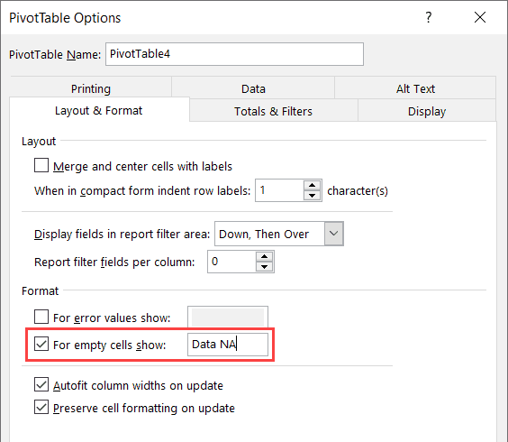
3. In the ‘PivotTable Options’ dialog box, click on the ‘Layout & Format’ tab
4. In the Format options, check the options and ‘For empty cells show:’ and leave it blank.
5. Click OK.

The above steps would hide the zeros in the Pivot Table and show a blank cell instead.

In case you want the Pivot Table to show something instead of the 0, you can specify that in step 4. For example, if you want to show the text – ‘Data not Available’, instead of the 0, type this text in the field (as shown below).

Find and Remove Zeros in Excel

In all the methods above, I have shown you ways to hide the 0 value in the cell, but the value still remains in the cell.

In case you want to remove the zero values from the dataset (which would leave you with blank cells), use the below steps:

1. Select the dataset (or the entire worksheet)
2. Click the Home tab
3. In the ‘Editing’ group, click on ‘Find & Select’
4. In the options that are shown in the drop-down, click on ‘Replace’
5. In the ‘Find and Replace’ dialog box, make the following changes:
   • In the ‘Find what’ field, enter 0
   • In the ‘Replace with’ field, enter nothing (leave it empty)
   • Click on Options button and check the ‘Match entire cell contents’ option
6. Click on Replace All

The above steps would instantly replace all the cells that had zero value with a blank.

In case you don’t want to remove the zeros right away and first select the cells, use the following steps:

1. Select the dataset (or the entire worksheet)
2. Click the Home tab
3. In the ‘Editing’ group, click on ‘Find & Select’
4. In the options that are shown in the drop-down, click on ‘Replace’
5. In the ‘Find and Replace’ dialog box, make the following changes:
   • In the ‘Find what’ field, enter 0
   • In the ‘Replace with’ field, enter nothing (leave it empty)
   • Click on Options button and check the ‘Match entire cell contents’ option
6. Click on the ‘Find All’ button. This will give you a list of all the cells that have 0 in it
7. Press Control-A (hold the control key and press A). This will select all the cells that have 0 in it.

Now, that you have all the cells with 0 selected, you can delete these, replace these with something else, or change the color and highlight these.

Hiding the Zeros Vs. Removing The Zeros

When treating the cells with 0s in it, you need to know the difference between hiding these and removing these.

When you hide the zero value in a cell, it is not visible to you, but it still remains in the cell. This means that if you have a dataset and you use it for calculation, that 0 value will also be used in the calculation.

On the contrary, when you have a blank cell, using it in formulas may mean that Excel automatically ignores these cells (depending on which formula you’re using).

For example, below is what I get when I use the AVERAGE formula to get the average for two columns (the result is in row 14). Column A has cells where the 0 value has been hidden (but is still there in the cell) and Column B has cells where the 0 value has been removed.

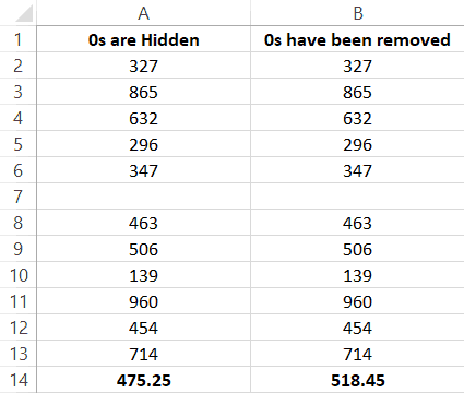
You can see the difference in the result despite the fact that the dataset for both datasets looks the same.

This happens as the AVERAGE formula ignores blank cells in column B, but it uses the ones in Column A (as the ones in column A still has the value 0 in it).

You may also like the following Excel tutorials:

• How to Hide a Worksheet in Excel
• Delete Rows Based on a Cell Value
• Delete Blank Rows in Excel
• How to Delete Every Other Row in Excel (or Every Nth Row)
• Show Formulas in Excel Instead of the Values
• Change Negative Number to Positive in Excel
• How to Remove Leading Zeros in Excel