
Содержание
- Using IF Function with Dates in Excel (Easy Examples)
- Syntax and Usage of the IF Function in Excel
- Comparing Dates in Excel (Using Operators)
- Using IF Function with Dates in Excel
- Using the IF Function with DATEVALUE Function
- Using the IF Function with the TODAY Function
- Using the IF Function with Future or Past Dates
- Points to Remember
- 3 thoughts on “Using IF Function with Dates in Excel (Easy Examples)”
- Excel IF Function With Dates
- Excel IF function combining with DATEVALUE function
- Excel IF function combining with DATE function
- Excel IF function combining with TODAY function
- IF statement in Excel with date1 and endtime variables
- 1 Answer 1
- How does the logical test in an Excel if statement evaluate dates in different formats?
- 1 Answer 1
- Excel IF Function – How to Use
- Definition of Excel IF Function
- Syntax
- Important Characteristics of IF Function in Excel
- Comparison Operators That Can Be Used With IF Statements
- Example 1: Using ‘equal to’ comparison operator within the IF function
- Example 2: Using ‘not equal to’ comparison operator within the IF function.
- Example 3: Using ‘less than’ operator within the IF function.
- Example 4: Using ‘greater than or equal to’ operator within the IF statement.
- Example 5: Using ‘greater than’ operator within the IF statement.
- Example 6: Using ‘less than or equal to’ operator within the IF statement.
- Example 7: Using an Excel Logical Function within the IF formula in Excel.
- Example 8: Using the Excel IF function to return another formula a result.
- Use Of AND & OR Functions or Logical Operators with Excel IF Statement
- Example 9: Using the IF function along with AND Function.
- Example 10: Using the IF function along with OR Function.
- Nested IF Statements
- Syntax:
- The above syntax translates to this:
- Example 11: Nested IF Statements
- Partial Matching or Wildcards with IF Function
- Example 12: Using FIND and SEARCH functions inside the IF statement
- Example 13: Using SEARCH function inside the Excel IF formula with wildcard operators
- Some Practical Examples of using the IF function
- Example 14: Using Excel IF function with dates.
- Example 15: Use an IF function-based formula to find blank cells in excel.
- Example 16: Use the Excel IF statement to show symbolic results (instead of textual results).
- IFS Function In Excel:
- Syntax for IFS function:
- Example 17: Using IFS function in Excel
- Subscribe and be a part of our 15,000+ member family!
Using IF Function with Dates in Excel (Easy Examples)
The IF function is one of the most useful Excel functions. It is used to test a condition and return one value if the condition is TRUE and another if it is FALSE.
One of the most common applications of the IF function involves the comparison of values.
These values can be numbers, text, or even dates. However, using the IF statement with date values is not as intuitive as it may seem.
In this tutorial, I will demonstrate some ways in which you can use the IF function with date values.
Table of Contents
Syntax and Usage of the IF Function in Excel
The syntax for the IF function is as follows:
- logical_test is the condition or criteria that you want the IF function to test. The result of this parameter is either TRUE or FALSE
- value_if_true is the value that you want the IF function to return if the logical_test evaluates to TRUE
- value_if_false is the value that you want the IF function to return if the logical_test evaluates to FALSE
For example, say you want to write a statement that will return the value “yes” if the value in cell reference A2 is equal to 10, and “no” if it’s anything but 10.
You can then use the following IF function for this scenario:

Comparing Dates in Excel (Using Operators)
Unlike numbers and strings, comparison operators, when used with dates, have a slightly different meaning.
Here are some of the comparison operators that you can use when comparing dates, along with what they mean:
| Operator | What it Means When Using with Dates |
|---|---|
| After the given date | |
| = | Same as or after the given date |
Using IF Function with Dates in Excel
It may look like IF formulas for dates are the same as IF functions for numeric or text values, since they use the same comparison operators.
However, it’s not as simple as that.
Unfortunately, unlike other Excel functions, the IF function cannot recognize dates.
It interprets them as regular text values.
So you cannot use a logical test such as “>05/07/2021” in your IF function, as it will simply see the value “05/07/2021” as text.
Here are a few ways in which you can incorporate date values into your IF function’s logical_test parameter.
Using the IF Function with DATEVALUE Function
If you want to use a date in your IF function’s logical test, you can wrap the date in the DATEVALUE function.
This function converts a date in text format to a serial number that Excel can recognize as a date.
If you put a date within quotes, it is essentially a text or string value.
When you pass this as a parameter to the DATEVALUE function, it takes a look at the text inside the double quotes, identifies it as a date and then converts it to an actual Excel date value.
Let us say you have a date in cell A2, and you want cell B2 to display the value “done” if the date comes before or on the same date as “05/07/2021” and display “not done” otherwise.
You can use the IF function along with DATEVALUE in cell B2 as follows:
Here’s a screenshot to illustrate the effect of the above formula:

Using the IF Function with the TODAY Function
If you want to compare a date with the current date, you can use the IF function with the TODAY function in the logical test.
Let’s say you have a date in cell A2 and you want cell B2 to display the value “done” if it is a date before today’s date.
If not, you want let’s say you want to display the value “not done”. You can use the IF function along with the TODAY function in cell B2 as follows:
Here’s a screenshot to illustrate the effect of the above formula (assuming the current date is 05/08/2021):

Using the IF Function with Future or Past Dates
An interesting thing about dates in Excel is that you can perform addition and subtraction operations with them too.
This is because dates are basically stored in Excel as serial numbers, starting from the date Jan 1, 1900.
Each day after that is represented by one whole number.
So, the serial number 2 corresponds to Jan 2, 1900, and so on.
This means that adding n number of days to a date is equivalent to adding the value n to the serial number that the date represents.
If TODAY() is 05/07/2021, then TODAY()+5 is five days after today, or 05/12/2021. Similarly, TODAY()-3 is three days before today or 05/04/2021.
Let’s say you have a date in cell A2 and you want cell B2 to mark it as “within range” if it is within 15 days from the current date.
If not, you want to show “out of range”. You can use the IF function along with the TODAY function in cell B2 as follows:
Here’s a screenshot to illustrate the effect of the above formula (assuming the current date is 05/08/2021):

Points to Remember
Having discussed different ways to use dates with the IF function, here are some important points to remember:
- Instead of hardcoding the dates into the IF function’s logical test parameter, you can store the date in a separate cell and refer to it with a cell reference. For example, instead of typing =IF(A2
3 thoughts on “Using IF Function with Dates in Excel (Easy Examples)”
Hi, can you identify the error here? “=If(G4=DATAVALUE(“1/0/1900″),”Email”,”No Email”)
Why isn’t this formula returning “Email”? Do I have to refer to the empty space (1/0/1900) as something else?
you have a typo. instead of “DATAVALUE” it should be “DATEVALUE”
What formula can I use to highlight a date that will expire soon but with a color, for example first aid course that will need renewing in 3 years time? thank you
Источник
Excel IF Function With Dates
If you have a list of dates and then want to compare to these dates with a specified date to check if those dates is greater than or less than that specified date. You can use the IF function in combination with logical operators and DATEVALUE function in Microsoft excel.
Excel IF function combining with DATEVALUE function
Since that Excel cannot recognize the date formats and just interprets them as a text string. So you need to use DATAVALUE function and let Excel think that it is a Date value. For example: DATEVALUE(“11/3/2018”). Now we can write down the following IF formula with Dates.
The above excel IF formula will check the date value in Cell B1 if it is less than another specified date(11/3/2018), if the test is TRUE, then return “good”, otherwise return “bad”
Excel IF function combining with DATE function
You can also use DATE function in an Excel IF statement to compare dates, like the below IF formula:
The above IF formula will check if the value in cell B1 is less than or equal to 11/3/2018 and show the returned value in cell C1, Otherwise show nothing.
Excel IF function combining with TODAY function
If you want to compare the current date with the specified date in the past, you can use IF function in combination with TODAY function in Excel. Like the following IF formula:
We also can use the complex logical test using Today function, like this: B1-TODAY>10, it will check the date value in one cell if it is more than 10 days from now. Let’s combine this logical test in the IF formula as follow:
Источник
IF statement in Excel with date1 and endtime variables
I have got an excel which has an formula and I am not able to understand how its working.
Here is the formula
Can someone spends few minutes to post an explanation, how it works
1 Answer 1
Try looking at it like this:
So the first thing checked is if the cell C6 equals date1, which I think is a named range. If they are equal, then the whole equation resolves to the next line, 0
If they are not equal then D6-endtime is evaluated, if it is less than or equal to zero, then the equation resolves to zero.
If D6-endtime is greater than 0, then the next test is true and the whole equation resolves to (D6-endtime)*1440 . There is no else in this last test because equation assumes D6-endtime will always be numeric.
Here’s how I understand IF statements work in excel =if(logical test,value if test true,value if test false) For logical test, you have to use something that resolves to TRUE or FALSE, or you can specify TRUE or FALSE directly(but then you don’t need an IF statement)
value if test true, if the test resolves to TRUE(like 1=1), then the cell will display this value, and supply this value to other functions
value if test false, if the test resolves to FALSE(like 1=0), then the cell will display this value, and supply this value to other functions.
You can omit value if TRUE/FALSE, and excel will return TRUE or FALSE after evaluation of the statement.
Источник
How does the logical test in an Excel if statement evaluate dates in different formats?
Spreadsheet with example data is linked here.
Suppose you have 3 dates «4/1/2015», «6/30/2015», and «5/1/2016» set to the Date cell format in Excel.
You can directly compare the dates using logical operators ( , etc.). If «4/1/2015» was in Cell A1 and «6/30/2015″ was in Cell A2, this formula =IF(A1>A2,»True»,»False») evaluates to «False».
However, you cannot compare a date against a string literal (i.e. «3/31/2015»). If «4/1/2015″ was in Cell A1, this formula =IF(AND(A1>=»4/01/2015»,A1 always evaluates to «False».
With the above noted, why is it that by appending an arithmetic operation to a string literal; Excel allows the comparison between dates stored in different formats? For example, if «4/1/2015» was in Cell A1, this formula =IF(AND(A1>=»4/01/2015″+0,A1 will evaluate to «True».
1 Answer 1
Dates are stored as a Double — the number of days from Dec 31, 1899 plus a fractional amount that is the percentage of time that has elapsed since midnight. Right now, I’m typing this at 42221.50049, which is 42,221 days since 1899 and a little after noon.
You see a date format only because you have a date format applied to that cell. It’s still a number underneath. But dates are a little special. The date also shows in Excel’s formula bar, not as a number, but as a date. Other formatted numbers don’t show this way. Excel is trying to walk a fine line between storing dates as Doubles and showing the user what they expect to see.
Excel has built-in type coercion. TC let’s you do things without being super rigorous about data types. Basically, if Excel can figure out how to do what you ask, it will do it. If you ask to add two strings, «1» + «1» Excel will coerce each of those strings to a number so it can perform the operation and give you 2 . If you ask «1» + «a» , you will get a #VALUE error because Excel can’t figure out how to coerce «a» into something that’s a valid operand.
Comparisons don’t trigger coercion. So =»1″=1 will return False — a string is not equal to a number and making the comparison does not trigger Excel to coerce either value to a different type.
In your case A1>=»04/01/2015″ seems like a great opportunity for Excel to coerce what looks like a date to an actual date. But it doesn’t. That’s just the way it works. But adding zero to the date (which remember is just a Double), coerces it into a date and you’re left comparing A1 to something that’s been coerced to a date.
String literals of dates seem to work in a lot of environments like SQL Server. But they generally don’t in Excel. It’s best, IMO, to use the DATE() function, as in A1>=DATE(2015,4,1) .
Источник
Excel IF Function – How to Use
IF function is undoubtedly one of the most important functions in excel. In general, IF statements give the desired intelligence to a program so that it can make decisions based on given criteria and, most importantly, decide the program flow.
In Microsoft Excel terminology, IF statements are also called «Excel IF-Then statements». IF function evaluates a boolean/logical expression and returns one value if the expression evaluates to ‘TRUE’ and another value if the expression evaluates to ‘FALSE’.
Table of Contents
Definition of Excel IF Function
According to Microsoft Excel, IF function is defined as a formula which «checks whether a condition is met, returns one value if true and another value if false».
Syntax
Syntax of IF function in Excel is as follows:
‘logic_test’ (required argument) – Refers to the boolean expression or logical expression that needs to be evaluated.
‘value_if_true’ (optional argument) – Refers to the value that will be returned by the IF function if the ‘logic_test’ evaluates to TRUE.
‘value_if_false’ (optional argument) – Refers to the value that will be returned by the IF function if the ‘logic_test’ evaluates to FALSE.

Important Characteristics of IF Function in Excel
- To use the IF function, you need to provide the ‘logic_test’ or conditional statement mandatorily.
- The arguments ‘value_if_true’ and ‘value_if_false’ are optional, but you need to provide at least one of them.
- The result of the IF statement can only be any one of the two given values (either it will be ‘value_if_true’ or ‘value_if_false’ ). Both values cannot be returned at the same time.
- IF function throws a ‘#Name?’ error if the ‘logic_test’ or boolean expression you are trying to evaluate is invalid.
- Nesting of IF statements is possible, but Excel only allows this to 64 levels. Nesting of IF statement means using one if statement within another.
Comparison Operators That Can Be Used With IF Statements
Following comparison operators can be used within the ‘logic_test’ argument of the IF function:
- = (equal to)
- <> (not equal to)
- (greater than)
- >= (greater than or equal to)
- Simple Examples of Excel IF Statement
Now, let’s try to see a simple example of the Excel IF function:
Example 1: Using ‘equal to’ comparison operator within the IF function
In this example, we have a list of colors, and we aim to find the ‘Blue’ color. If we are able to find the ‘Blue’ color, then in the adjacent cell, we need to assign a ‘Yes’; otherwise, assign a ‘No’.

So, the formula would be:
This suggests that if the value present in cell A2 is ‘Blue’, then return a ‘Yes’; otherwise, return a ‘No’.
If we drag this formula down to all the rows, we will find that it returns ‘Yes’ for the cells with the value ‘Blue’ for all others; it would result in ‘No’.
Example 2: Using ‘not equal to’ comparison operator within the IF function.
Let’s take example 1, and understand how we can reverse the logic and use a ‘not equal to’ operator to construct the formula so that it still results in ‘Yes’ for ‘Blue’ color and ‘No’ for any other text.

So the formula would be:
This suggests that if the value at A2 is not equal to ‘Blue’, then return a ‘No’; otherwise, return a ‘Yes’.
When dragged down to all the below rows, this formula would find all the cells (from A2 to A8) where the value is not ‘Blue’ and marks a ‘No’ against them. Otherwise, it marks a ‘Yes’ in the adjacent cells.
Example 3: Using ‘less than’ operator within the IF function.
In this example, we have scores of some students, along with their names. We want to assign either «Pass» or «Fail» against each student in the result column.

Based on our criteria, the passing score is 50 or more.
For this, we can use the IF function as:
This suggests that if the value at B2, i.e., 37, is less than 50, then return «Fail»; otherwise, return «Pass».
As 37 is less than 50 so the result will be «Fail».
We can drag the above-given formula for the rest of the cells below and the result would be correct.
Example 4: Using ‘greater than or equal to’ operator within the IF statement.
Let’s take example 3 and see how we can reverse the logic and use a ‘greater than or equal to’ operator to construct the formula so that it still results in ‘Pass’ for scores of 50 or more and ‘Fail’ for all the other scores.

For this, we can use the Excel IF function as:
This suggests that if the value at B2, i.e., 37 is greater than or equal to 50, then return «Pass»; otherwise, return «Fail».
As 37 not greater than or equal to 50 so the result will be «Fail».
When dragged down for the rest of the cells below, this formula would assign the correct result in the adjacent rows.
Example 5: Using ‘greater than’ operator within the IF statement.
In this example, we have a small online store that gives a discount to its customers based on the amount they spend. If a customer spends $50 or more, he is applicable for a 5% discount; otherwise, no discounts are offered.

To find whether a discount is offered or not, we can use the following excel formula:
This translates to – If the value at B2 cell is greater than 50, assign a text «5% Discount» otherwise, assign a text «No Discount» against the customer.
In the first case, as 23 is not greater than 50, the output will be «No Discount».
We can drag the above-given formula for the rest of the cells below are the result would be correct.
Example 6: Using ‘less than or equal to’ operator within the IF statement.
Let’s take example 5 and see how we can reverse the logic and use a ‘less than or equal to’ operator to construct the formula so that it still results in a ‘5% Discount’ for all customers whose total spend exceeds $50 and ‘No Discount’ for all the other customers.

For this, we can use the IF-then statement as:
This means that if the value at B2, i.e., 23, is less than or equal to 50, then return «No Discount»; otherwise, return «5% Discount».
As 23 is less than or equal to 50 so the result will be «No Discount».
When dragged down for the rest of the cells below, this formula would assign the correct result in the adjacent rows.
Example 7: Using an Excel Logical Function within the IF formula in Excel.
In this example, let’s suppose we have a list of numbers, and we have to mark Even and Odd numbers. We can do this using the IF condition and the ISEVEN or ISODD inbuilt functions provided by Microsoft Excel.
ISEVEN function returns ‘true’ if the number passed to it is even; otherwise, it returns a ‘false’. Similarly, ISODD function return ‘true’ if the number passed to it is odd; otherwise, it returns a ‘false’.

For this, we can use the IF-then statement as:
This means that – If the value at A2 cell is an even number, then the result would be «Even»; otherwise, the result would be «Odd».
Alternatively, the above logic can also be written using the ISODD function along with the IF statement as:
This means that – If the value at A2 cell is an odd number, then the result would be «Odd»; otherwise, the result would be «Even».
Example 8: Using the Excel IF function to return another formula a result.
In this example, we have Employee Data from a company. The company comes up with a simple way to reward its loyal employees. They decide to give the employees an annual bonus based on the years spent by the employee within the organization.
Employees with experience of more than 5 years are given 10% of annual salary as a bonus whereas everyone else gets a 5% of annual salary as a bonus.

For this, the excel formula would be:
This means that – if the value at B2 (experience column) is greater than 5, then return a result by calculating 10% of C2 (annual salary column). However, if the logic test is evaluated to false, then return the result by calculating 5% of C2 (annual salary column)
Use Of AND & OR Functions or Logical Operators with Excel IF Statement
Excel IF Statement can also be used along with the other functions like AND, OR, NOT for analyzing complex logic. These functions (AND, OR & NOT) are called logical operators as they are used for connecting two or more logical expressions.
AND Function– AND function returns true when all the conditions inside the AND function evaluate to true. The syntax of AND Function in Excel is:
OR Function– OR function returns true when any one of the conditions inside the OR function evaluates to true. The syntax of OR Function in Excel is:
Example 9: Using the IF function along with AND Function.
In this example, we have Math and science test scores of some students, and we want to assign a ‘Pass’ or ‘Fail’ value against the students based on their scores.
Passing criteria: Students have to get more than 50 marks in Math and more than 70 marks in science to pass the test.

Based on the above conditions, the formula would be:
The formula translates to – if the value at B2 (Math score) is greater than 50 and the value at C2 (Science Score) is greater than 70, then assign the value «Pass»; otherwise, assign the value «Fail».
Example 10: Using the IF function along with OR Function.
In this example, we have two test scores of some students, and we want to assign a ‘Pass’ or ‘Fail’ value against the students based on their scores.
Passing criteria: Students have to clear either one of the two tests with more than 50 marks.

Based on the above conditions, the formula would be:
The formula translates to – if either the value at B2 (Test 1 score) is greater than 50, OR the value at C2 (Test 2 Score) is greater than 50, then assign the value «Pass»; otherwise, assign the value «Fail».
Nested IF Statements
When used alone, IF formula can only result in two outcomes, i.e., True or False. But there are many cases when we want to test multiple outcomes with IF statement.
In such cases, nesting two or more IF Then statements one inside another can be convenient in writing formulas.
Syntax:
The syntax of the Nested IF Then statements is as follows:
‘condition_1’ – Refers to the first logical test or conditional expression that needs to be evaluated by the outer IF function.
‘value_if_true_1’ – Refers to the value that will be returned by the outer IF function if the ‘condition_1’ evaluates to TRUE.
‘condition_2’ – Refers to the second logical test or conditional expression that needs to be evaluated by the inner IF function.
‘value_if_true_2’ – Refers to the value that will be returned by the inner IF function if the ‘condition_2’ evaluates to TRUE.
‘value_if_false_2’ – Refers to the value that will be returned by the inner IF function if the ‘condition_2’ evaluates to FALSE.
The above syntax translates to this:
As we can see, Nested formulas can quickly become complicated so, let’s try to understand how nesting of the IF statement works with an example.
Example 11: Nested IF Statements
In this example, we have a list of countries and their average temperatures in degree Celsius for the month of January. Our goal is to categorize the country based on the temperature range as follows:
Criteria: Temperatures below 20 °C should be marked as «Below Room Temperature», temperatures between 20°C to 25°C should be classified as «Normal Room Temperature», whereas any temperature over 25°C should be marked as «Above Room Temperature».

Based on the above conditions, the formula would be:
The formula translates to – if the value at B2 is less than 20, then the text «Below Room Temperature» is returned from the outer IF block. However, if the value at B2 is greater than or equal to 20, then the inner IF block is evaluated.
Inside the inner IF block, the value at B2 is checked. If the value at B2 is greater than or equal to 20 and less than or equal to 25. Then the inner IF block returns the text «Normal Room Temperature».
However, if the condition inside the inner IF block also evaluates to ‘false’ that means the value at B2 is greater than 25, so the result will be «Above Room Temperature».
Partial Matching or Wildcards with IF Function
Although IF function itself doesn’t accept any wildcard characters like (* or ?) while performing the logic test, thankfully, there are ways to perform partial matching and wildcard searches with the IF function.
To perform partial matching inside the IF function, we can use the FIND (case sensitive) or SEARCH (case insensitive) functions.
Let’s have a look at this with some examples.
Example 12: Using FIND and SEARCH functions inside the IF statement
In this example, we have a list of customers, and we need to find all the customers whose last name is «Flynn». If the customer name contains the text «Flynn», then we need to assign a text «Found» against their names. Otherwise, we need to assign a text «Not Found».

For this, we can make use of the FIND function within the IF function as:
Using the FIND function, we perform a case-sensitive search of the text «Flynn» within the customer name column. If the FIND function is able to find the text «Flynn», it returns a number signifying the position where it found the text.
If the number returned by the FIND function is valid, the ISNUMBER Function returns a value true. Else, it returns false. Based on the ISNUMBER function’s output, the logic test is performed and the appropriate value «Found» or «Not Found» is assigned.
Note: It should be noted that the FIND function performs a case-sensitive search.
This means in the above example if the customer name is entered in lower case (like «sean flynn» then the above function would return not found against them.
To perform a case-insensitive search, we can replace the find function with the search function, and the rest of the formula would be the same.
Example 13: Using SEARCH function inside the Excel IF formula with wildcard operators
In this example, we have the same customer list from example 12, and we need to find all the customers whose name contains «M». If the customer name contains the alphabet «M», we need to assign a text «M Found» against their names. Otherwise, we need to assign a text «M Not Found».

For this, we can use the SEARCH function with a wildcard ‘*’ operator inside the IF function as:
For more details on Search Function and wildcard, operators check out this article – Search Function In Excel
Some Practical Examples of using the IF function
Now, let’s have a look at some more practical examples of the Excel IF Function.
Example 14: Using Excel IF function with dates.
In this example, we have a task list along with the task due dates. Our goal is to show results based on the task due date.
If the task due date was in the past, we need to show «Was due <1,2,3..>day(s) back», if the task due date is today’s date, we need to show «Today» and similarly, if the task due date is in the future then we need to show «Due in <1,2,3..>day(s)»

In Microsoft Excel, we can do this with the help of the IF-then statement and TODAY function, as shown below:
This means that – compare the date present in cell B2 if the date is equal to today’s date show the text «Today». If the date in cell B2 is not equal to today’s date, then the inner IF block checks if the date in B2 is greater than today’s date. If the date in cell B2 is greater than today’s date, that means the date is in the future, so show the text «Due in <1,2,3…>days».
However, if the date in cell B2 is not greater than today’s date, that means the date was in the past; in such a case, show the text «Was due <1,2,3..>day(s) back».
You can also go a step further and apply conditional formatting on the range and highlight all the cells with the text «Today!». This will help you to clearly see
Example 15: Use an IF function-based formula to find blank cells in excel.
In this example, we will use the IF function to find the blank cells in Microsoft Excel. We have a list of customers, and in between the list, some of the cells are blank. We aim to find the blank cells and add the text «blank call found!» against them.

We can do this with the help of the IF function along with the ISBLANK function. The ISBLANK function returns a true if the cell reference passed to it is blank. Otherwise, the ISBLANK function returns false.
Let’s see the formula –
This means that – If the cell at A2 is blank, then the resultant text should be «Blank cell found!», however, if the cell at A2 is not blank, then don’t show any text.
Example 16: Use the Excel IF statement to show symbolic results (instead of textual results).
In this example, we have a list of sales employees of a company along with the number of products sold by the employees in the current month. We want to show an upward arrow symbol (↑) if the employee has done more than 50 sales and a downward arrow symbol (↓) if the employee has made less than 50 sales.

To do this, we can use the formula:
This implies – If the value at B2 is greater than 50, then, as a result, show the content in cell G6 (cell containing upward arrow) and otherwise show the content at G8 (cell containing downward arrow)
If you wonder about the ‘$’ signs used in the formula, you can check out this post – Excel Absolute References . These ‘$’ symbols are used for making excel cell references absolute.
IFS Function In Excel:
IFS Function in Microsoft Excel is a great alternative to nested IF Statements. It is very similar to a switch statement. The IFS function evaluates multiple conditions passed to it and returns the value corresponding to the first condition that evaluates to true.
IFS function is a lot simple to write and read than nested IF statements. IFS function is available in Office 2019 and higher versions.
Syntax for IFS function:
‘test1’ (required argument) – Refers to the first logical test that needs to be evaluated.
‘value1’ (required argument) – Refers to the result to be returned when ‘test1’ evaluates to TRUE.
‘test2’ (optional argument) – Refers to the second logical test that needs to be evaluated
‘value2’ (optional argument) – Refers to the result to be returned when ‘test2’ evaluates to TRUE.
Example 17: Using IFS function in Excel
In this example, we have a list of students, along with their scores, and we need to assign a grade to the students based on the scores.
The grading criteria is as follows – Grade A for a score of 90 or more, Grade B for a score between 80 to 89.99, Grade C for a score between 70 to 79.99, Grade D for a score between 60 to 69.99, Grade E for a score between 60 to 59.99, Grade F for a score lower than 50.

Let’s see how easily write such a complicated formula with the IFS function:
This implies that – If B2 is greater than or equal to 90, return A. Else if B2 is greater than or equal to 80, return B. Else if B2 is greater than or equal to 70, return C. Else if B2 is greater than or equal to 60, return D. Else if B2 is greater than or equal to 50, return E. Else if B2 is less than 50, return F.
If you would try to write the same formula using nested IF statements, see how long and complicated it becomes:
So, this was all about the IF function in excel. If you want to learn more about IF function, I would recommend you to go through this article – VBA IF Statement With Examples
Subscribe and be a part of our 15,000+ member family!
Now subscribe to Excel Trick and get a free copy of our ebook «200+ Excel Shortcuts» (printable format) to catapult your productivity.
Источник
Explanation
In this example, the goal is to check if a given date is between two other dates, labeled «Start» and «End» in the example shown. For convenience, both start (E5) and end (E8) are named ranges. If you prefer not to use named ranges, make sure you use absolute references for E5 and E8.
Excel dates
Excel dates are just large serial numbers and can be used in any numeric calculation or comparison. This means we can simply compare a date to another date with a logical operator like greater than or equal (>=) or less than or equal (<=).
AND function
The main task in this example is to construct the right logical test. The first comparison is against the start date. We want to check if the date in B5 is greater than or equal (>=) to the date in cell E5, which is the named range start:
=B5>=start
The second expression needs to check if the date in B5 is less than or equal (<=) to the end date in cell E5:
=B5<=end
The goal is to check both of these conditions are TRUE at once, and for that, we use the AND function:
=AND(B5>=start,B5<=end) // returns TRUE or FALSE
The AND function will return TRUE when the date in B5 is greater than or equal to start AND less than equal to end. If either test fails, the AND function will return FALSE. We now have the logic we need to use with the IF function.
IF function
We start off by placing the expression above inside the IF function as the logical_test argument:
=IF(AND(B5>=start,B5<=end)
Next, we add a value_if_true argument. In this case, we want to return an «x» when a date is between two dates, so we add «x» as a text value:
=IF(AND(B5>=start,B5<=end),"x"
If the date in B5 is not between start and end, we don’t want to display anything, so we use an empty string («») for value_if_false. The final formula in C5 is:
=IF(AND(B5>=start,B5<=end),"x","")
As the formula is copied down, the formula returns «x» if the date in column B is between the start and end date. If not, the formula returns an empty string («»), which looks like an empty cell in Excel. The values returned by the IF function can be customized as desired.
Try looking at it like this:
=IF(C6=date1,
        0,
        IF(D6-endtime<=0,
                0,
                IF(D6-endtime>0,
                          (D6-endtime)*1440
                          #no "else statement" here!
                 )
        )
)
So the first thing checked is if the cell C6 equals date1, which I think is a named range. If they are equal, then the whole equation resolves to the next line, 0
If they are not equal then D6-endtime is evaluated, if it is less than or equal to zero, then the equation resolves to zero.
If D6-endtime is greater than 0, then the next test is true and the whole equation resolves to (D6-endtime)*1440. There is no else in this last test because equation assumes D6-endtime will always be numeric.
Here’s how I understand IF statements work in excel
=if(logical test,value if test true,value if test false)
For logical test, you have to use something that resolves to TRUE or FALSE, or you can specify TRUE or FALSE directly(but then you don’t need an IF statement)
value if test true, if the test resolves to TRUE(like 1=1), then the cell will display this value, and supply this value to other functions
value if test false, if the test resolves to FALSE(like 1=0), then the cell will display this value, and supply this value to other functions.
You can omit value if TRUE/FALSE, and excel will return TRUE or FALSE after evaluation of the statement.
The IF function is one of the most flexible functions in Microsoft Excel and has a range of uses that can be helpful in comparing data entries and isolating specific data points. The IF function can be used to evaluate both dates and text in Microsoft Excel and this article will teach you how to do so.
To use IF functions with dates and text:
Let’s take the example of a school administrator who is trying to group together classes for the upcoming year. The administrator needs to split students into three different classrooms, based on their dates of birth. If a student is born between 01/01/1994 and 31/12/1995, he or she will be assigned to room U16; if he or she is born between 01/01/1996 and 31/12/1997, he or she will be assigned to U14; and if the student’s birth date is later than 01/01/1998, he or she will be assigned to U12 .
Assuming that your date entry is in A1, the following formula would apply. (Note that all dates are entered in mm/dd/yy format):
=IF(AND(A1>="1/1/94"+0,A1<="12/31/95"+0),"U16",IF(AND(A1>="1/1/96"+0,A1<="12/31/97"+0),"U14",IF(A1>=1/1/98,"U12","")))
All text entries in this example would be placed into column B2. Depending on the actual input cell of your data, you can easily change each instance where A1 is found.
Any more Excel questions? Check out our forum!
Updated 12/16/22: Stay up to date on the latest from Excel and download Excel templates today.
Date functions in Microsoft Excel make it possible to perform date calculations, like addition or subtraction, resulting in automated or semi-automated worksheets. The NOW function, which calculates values based on the current date and time, is a great example of this.
Taking this functionality a step further, when you mix date functions with conditional formatting, you can create spreadsheets that display date alerts automatically when a deadline is near or differentiates between types of days, like weekends and weekdays.

Get a better picture of your data.
The basics of conditional formatting for dates
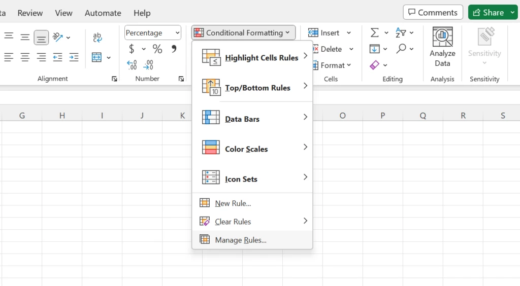
To find conditional formatting for dates, go to:
Home > Conditional Formatting > Highlight Cell Rules > A Date Occurring.
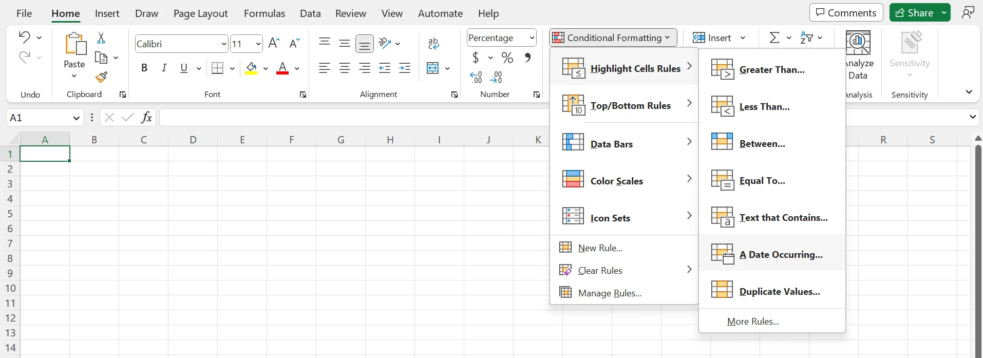
You can select the following date options, ranging from yesterday to next month:
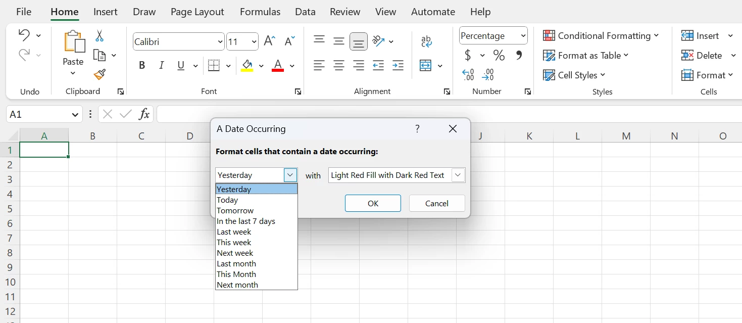
These 10 date options generate rules based on the current date. If you need to create rules for other dates (e.g., greater than a month from the current date), you can create your own new rule.
Below are step-by-step instructions for a few of my favorite conditional formats for dates.
Highlighting weekends
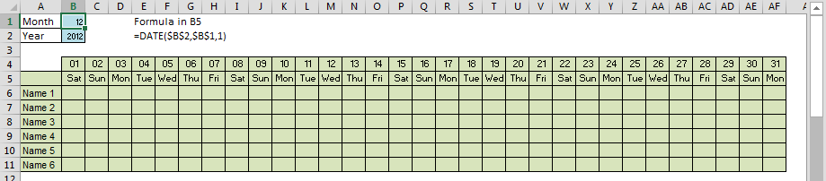
When you design an automated calendar you don’t need to color the weekends yourself. With the conditional formatting tool, you can automatically change the colors of weekends by basing the format on the WEEKDAY function. Assume that you have the date table—a calendar without conditional formatting:
To change the color of the weekends, open the menu Conditional Formatting > New Rule.

In the next dialog box, select the menu Use a formula to determine which cell to format.
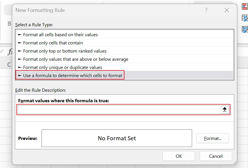
In the text box Format values where this formula is true, enter the following WEEKDAY formula to determine whether the cell is a Saturday (6) or Sunday (7):
=WEEKDAY(B$5,2)>5
Parameter 2 means Saturday = 6 and Sunday = 7. This parameter is very useful to test for weekends.
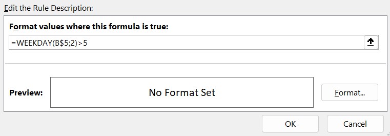
Note: In this case, you must lock the reference of the row so that the conditional format will work correctly in the other cells in this table.
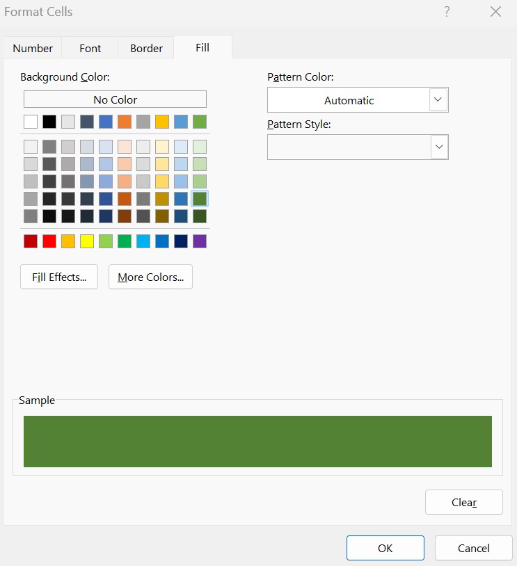
Then, customize the format of your condition by clicking on the Format button and you choose a fill color (orange in this example).
format numbers as dates <br>or times in Excel
Learn more
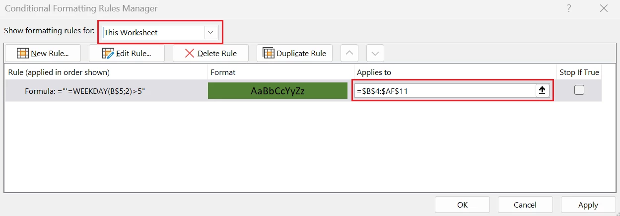
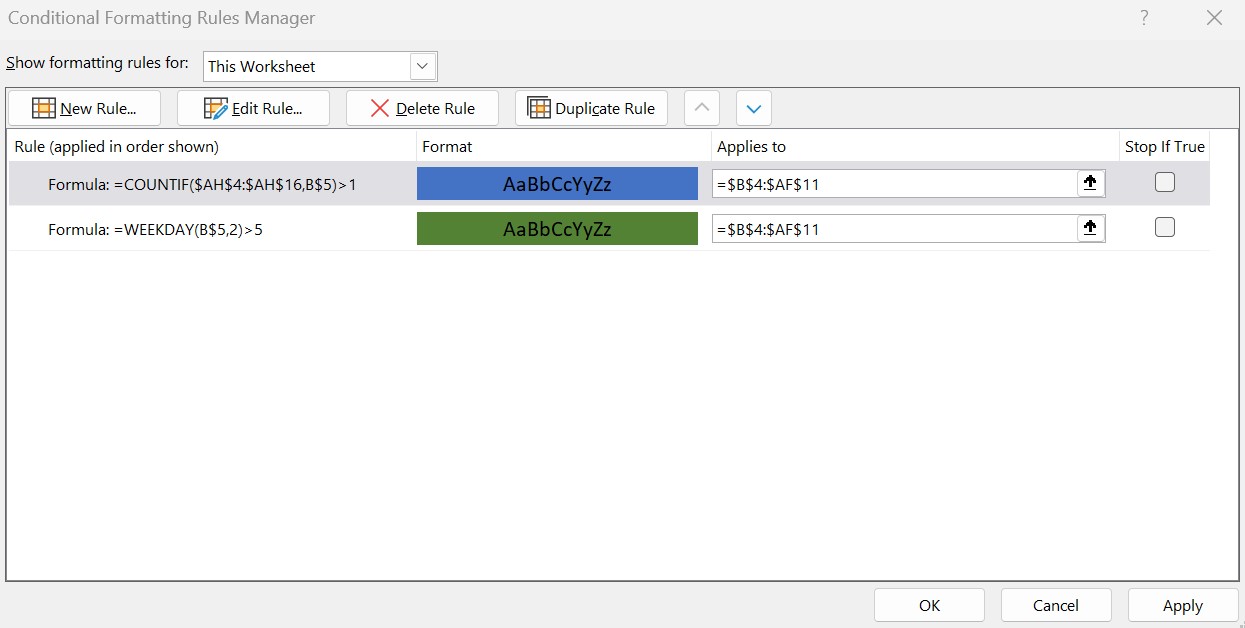
Click OK, then open Conditional Formatting> Manage Rules.
Select This Worksheet to see the worksheet rules instead of the default selection. In Applies to, change the range that corresponds to your initial selection when creating your rules to extend it to the whole column.
Now you will see a different color for the weekends. Note: This example shows the result in the Excel Web App.
Highlighting holidays
To enrich the previous workbook, you could also color-code holidays. To do that, you need a column with the holidays you’d like to highlight in your workbook (but not necessarily in the same sheet). In our example, we have US public holidays in column AH (as related to the year in cell B2).
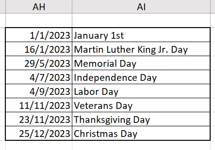
Again, open the menu Conditional Formatting > New Rule. In this case, we use the formula COUNTIF in order to count if the number of public holidays in the current month is greater than 1.
=COUNTIF($AH$4:$AH$16,B$5)>1
Then, in the dialog box Manage Rules, select the range B4:AF11. If you want to highlight the holidays over the weekends, you move the public holiday rule to the top of the list.
This example in the Excel Web App shows the result. Change the value of the month and the year to see how the calendar has a different format.
Highlighting delays
In case we want to change the color of cells based on our approach on a date again, we will use conditional formatting to make it work for us.
In the following example, we show:
- Yellow dates between 1 and 2 months.
- Orange dates between 2 and 3 months.
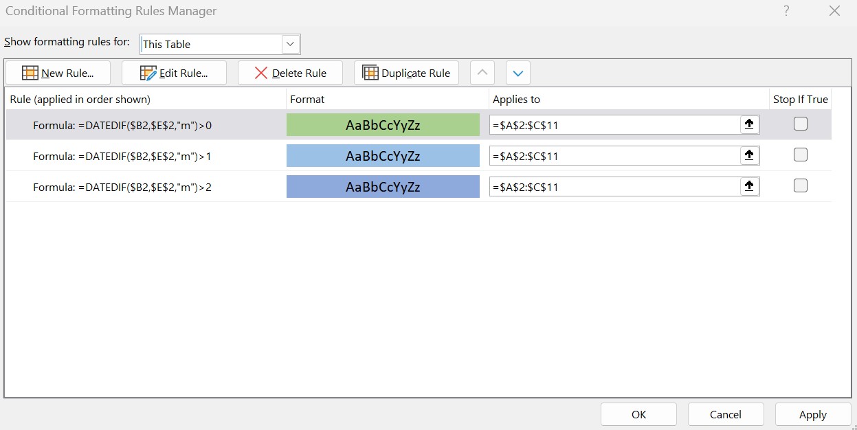
- Purple dates more than 3 months.
We then construct three rules of conditional formatting using the formula DATEDIF. Respectively for the three cases the following formulas:
=DATEDIF($B2,$E$2,”m”)>0
=DATEDIF($B2,$E$2,”m”)>1
=DATEDIF($B2,$E$2,”m”)>2
In the Excel Web App, try changing some dates to experiment with the result.

Task management in Microsoft 365
Collaborate on shared Office documents, including Excel, Word, and PowerPoint.
Color scales
Rather than choose a different color set for each period in our timeframe, we will work with the option of color scales to color our cells.
First, go into a new column (column E) and calculate the difference in the number of days in a year again with the DATEDIF formula and the parameter “yd”.
=DATEDIF($D2,TODAY(),”yd”)
Then choose the menu Conditional Formatting> New Rule option Format all cells based on their value and choose the following options:
- Scale = 3 colors
- Minimum = 0 Green
- Midpoint = 10 White
- Maximum = 30 Blue
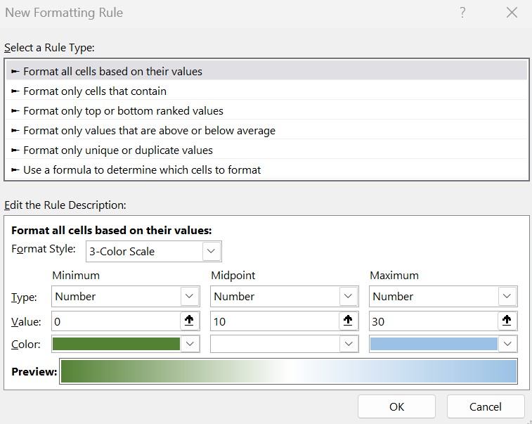
The result is a gradient color scale with nuances from green to white and through blue. The closer to 0 the more green, the closer to 10 the more white, and the closer to 30 the more blue. In the Excel app, try changing some dates to experiment with the result.
Learn more
Explore Microsoft Excel today.
Additional resources:
- Read more about the DATE function.
- Read how to format numbers as dates and times.