If statement in excel with and or not

The logical IF statement in Excel is used for the recording of certain conditions. It compares the number and / or text, function, etc. of the formula when the values correspond to the set parameters, and then there is one record, when do not respond — another.

Logic functions — it is a very simple and effective tool that is often used in practice. Let us consider it in details by examples.



The syntax of the function «IF» with one condition

The operation syntax in Excel is the structure of the functions necessary for its operation data.

=IF(boolean;value_if_TRUE;value_if_FALSE)

Let us consider the function syntax:

• Boolean – what the operator checks (text or numeric data cell).
• Value_if_TRUE – what will appear in the cell when the text or numbers correspond to a predetermined condition (true).
• Value_if_FALSE – what appears in the box when the text or the number does not meet the predetermined condition (false).

Example:

Logical IF functions.

The operator checks the A1 cell and compares it to 20. This is a «Boolean». When the contents of the column is more than 20, there is a true legend «greater 20». In the other case it’s «less or equal 20».

Attention! The words in the formula need to be quoted. For Excel to understand that you want to display text values.

Here is one more example. To gain admission to the exam, a group of students must successfully pass a test. The results are listed in a table with columns: a list of students, a credit, an exam.

The statement IF should check not the digital data type but the text. Therefore, we prescribed in the formula В2= «done» We take the quotes for the program to recognize the text correctly.



The function IF in Excel with multiple conditions

Usually one condition for the logic function is not enough. If you need to consider several options for decision-making, spread operators’ IF into each other. Thus, we get several functions IF in Excel.

The syntax is as follows:

Here the operator checks the two parameters. If the first condition is true, the formula returns the first argument is the truth. False — the operator checks the second condition.

Examples of a few conditions of the function IF in Excel:

It’s a table for the analysis of the progress. The student received 5 points:

• А – excellent;
• В – above average or superior work;
• C – satisfactory;
• D – a passing grade;
• E – completely unsatisfactory.

IF statement checks two conditions: the equality of value in the cells.

In this example, we have added a third condition, which implies the presence of another report card and «twos». The principle of the operator is the same.

Enhanced functionality with the help of the operators «AND» and «OR»

When you need to check out a few of the true conditions you use the function И. The point is: IF A = 1 AND A = 2 THEN meaning в ELSE meaning с.

OR function checks the condition 1 or condition 2. As soon as at least one condition is true, the result is true. The point is: IF A = 1 OR A = 2 THEN value B ELSE value C.

Functions AND & OR can check up to 30 conditions.

An example of using the operator AND:

It’s the example of using the logical operator OR.

How to compare data in two tables

Users often need to compare the two spreadsheets in an Excel to match. Examples of the «life»: compare the prices of goods in different bringing, to compare balances (accounting reports) in a few months, the progress of pupils (students) of different classes, in different quarters, etc.

To compare the two tables in Excel, you can use the COUNTIFS statement. Consider the order of application functions.

For example, consider the two tables with the specifications of various food processors. We planned allocation of color differences. This problem in Excel solves the conditional formatting.

Baseline data (tables, which will work with):

Select the first table. Conditional Formatting — create a rule — use a formula to determine the formatted cells:

In the formula bar write: = COUNTIFS (comparable range; first cell of first table)=0. Comparing range is in the second table.

To drive the formula into the range, just select it first cell and the last. «= 0» means the search for the exact command (not approximate) values.

Choose the format and establish what changes in the cell formula in compliance. It’s better to do a color fill.

Select the second table. Conditional Formatting — create a rule — use the formula. Use the same operator (COUNTIFS). For the second table formula:

Download all examples in Excel

Now it is easy to compare the characteristics of the data in the table.

The beauty of Excel lies in its flexibility to create pretty much any mathematical model with little effort. Logic gates can be established within a table, chart, or any other spreadsheet element to dissect data and results. This gives Excel users the ability to create advanced data models. In the heart of logic statements lie 4 functions, IF, AND, OR, and NOT. Using these alone, you can automate data. In this article, we’re going to be focusing on their basics, and how to use them. You can download our spreadsheet template below.

IF

Once of the most popular function in Excel, the IF function, checks a logical statement, and returns a value based on the result. This function has 3 arguments and its parameters are,

=IF(do this logical test, if the answer is true – do this, if answer is false – do this)

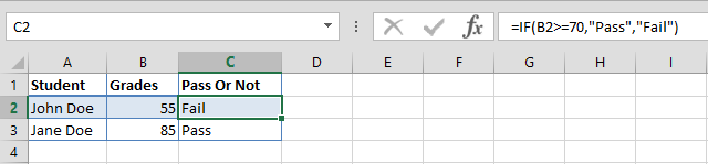
Any ‘do this or that’ situation can be given as an example. Here, we created a list of students and their grades. Let’s try to find out who passed and who failed the test. If the grade is equal to or greater than 70 (B2>=70) it’s a pass, otherwise a fail. We can also have Excel print “Pass” if this statement is true and “Fail” if not. The formula then becomes,

=IF(B2>=70,»Pass»,»Fail»)

AND — OR — NOT

IF isn’t the only function that can be used to run logical tests. For when there’s more the than one condition, there are other functions we can utilize. The most common examples are the AND, OR and NOT functions.

These functions, just like the IF function, evaluate a logical statement, and return values based on the outcome. This makes them really handy when using in conjunction with the logical test portion of an IF function. You can think of them as math operators.

• AND returns TRUE only if every argument is true, otherwise gives FALSE.
• OR returns TRUE if any argument is TRUE; if every arguments are FALSE, returns FALSE.
• NOT returns the opposite logical value of the argument. TRUE to FALSE and FALSE to TRUE.

Let’s take a closer look at each function.

AND

In an alternative scenario, let’s say the students have a total of 3 grades, from 2 exams and a final. A student can pass only if each individual grade is greater than or equal to 60. Here our rule is, «all grades should be greater than or equal to 60”. We can use the AND function to combine these requirements,

=IF(AND(B7>=60,C7>=60,D7>=60),»Pass»,»Fail»)

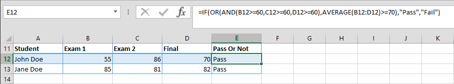
OR

Let’s take a different case. If either one rule below was enough for a pass grade, we could utilize the OR function.

1. All grades should be equal to or greater than 60 (AND(B7>=60,C7>=60,D7>=60))

OR

1. Average of grades should be equal to or greater than 70 (AVERAGE(B7:D7)>=70)

The statement becomes,

=IF(OR(AND(B7>=60,C7>=60,D7>=60),AVERAGE(B7:D7)>=70),»Pass»,»Fail»)

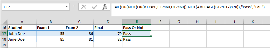
NOT

When you need to include all results but a certain rule, the NOT function is the best way to go. For example, “All grades should be equal to or greater than 60” statement can be defined as,

=NOT(OR(B17<60,C17<60,D17<60))

This statement will check for any grade that is less than 60. For those that are, the formula returns the opposite parameter (FALSE) because that is the “Fail” condition for this scenario. Looking for a Pass/Fail, the full statement would be as follows,

=IF(OR(NOT(OR(B17<60,C17<60,D17<60)),NOT(AVERAGE(B17:D17)<70)),»Pass»,»Fail»)