If starts with excel 2010 - Word и Excel - помощь в работе с программами

IF function

The IF function is one of the most popular functions in Excel, and it allows you to make logical comparisons between a value and what you expect.

So an IF statement can have two results. The first result is if your comparison is True, the second if your comparison is False.

For example, =IF(C2=”Yes”,1,2) says IF(C2 = Yes, then return a 1, otherwise return a 2).

Use the IF function, one of the logical functions, to return one value if a condition is true and another value if it’s false.

IF(logical_test, value_if_true, [value_if_false])

For example:

=IF(A2>B2,»Over Budget»,»OK»)
=IF(A2=B2,B4-A4,»»)

Argument name	Description
logical_test (required)	The condition you want to test.
value_if_true (required)	The value that you want returned if the result of *logical_test* is TRUE.
value_if_false (optional)	The value that you want returned if the result of *logical_test* is FALSE.

Simple IF examples

=IF(C2=”Yes”,1,2)

In the above example, cell D2 says: IF(C2 = Yes, then return a 1, otherwise return a 2)

=IF(C2=1,”Yes”,”No”)

In this example, the formula in cell D2 says: IF(C2 = 1, then return Yes, otherwise return No)As you see, the IF function can be used to evaluate both text and values. It can also be used to evaluate errors. You are not limited to only checking if one thing is equal to another and returning a single result, you can also use mathematical operators and perform additional calculations depending on your criteria. You can also nest multiple IF functions together in order to perform multiple comparisons.

=IF(C2>B2,”Over Budget”,”Within Budget”)

In the above example, the IF function in D2 is saying IF(C2 Is Greater Than B2, then return “Over Budget”, otherwise return “Within Budget”)

=IF(C2>B2,C2-B2,0)

In the above illustration, instead of returning a text result, we are going to return a mathematical calculation. So the formula in E2 is saying IF(Actual is Greater than Budgeted, then Subtract the Budgeted amount from the Actual amount, otherwise return nothing).

=IF(E7=”Yes”,F5*0.0825,0)

In this example, the formula in F7 is saying IF(E7 = “Yes”, then calculate the Total Amount in F5 * 8.25%, otherwise no Sales Tax is due so return 0)

Note: If you are going to use text in formulas, you need to wrap the text in quotes (e.g. “Text”). The only exception to that is using TRUE or FALSE, which Excel automatically understands.

Common problems

Problem	What went wrong
0 (zero) in cell	There was no argument for either value_if_true or value_if_False arguments. To see the right value returned, add argument text to the two arguments, or add TRUE or FALSE to the argument.
#NAME? in cell	This usually means that the formula is misspelled.

Need more help?

You can always ask an expert in the Excel Tech Community or get support in the Answers community.

I know this is a really old post, but I found it in searching for a solution to the same problem. I don’t want a nested if-statement, and Switch is apparently newer than the version of Excel I’m using. I figured out what was going wrong with my code, so I figured I’d share here in case it helps someone else.

I remembered that VLOOKUP requires the source table to be sorted alphabetically/numerically for it to work. I was initially trying to do this…

=LOOKUP(LOWER(LEFT($T$3, 1)),  {"s","l","m"}, {-1,1,0})

and it started working when I did this…

=LOOKUP(LOWER(LEFT($T$3, 1)),  {"l","m","s"}, {1,0,-1})

I was initially thinking the last value might turn out to be a default, so I wanted the zero at the last place. That doesn’t seem to be the behavior anyway, so I just put the possible matches in order, and it worked.

Edit: As a final note, I see that the example in the original post has letters in alphabetical order, but I imagine the real use case might have been different if the error was happening and the letters A, B, and C were just examples.

Источник

In this article, we will learn how to Check values which start with either A, B or C using wildcards in Excel.
In simple words, while working with table values, sometimes we need to check the value in cell whether it starts with A, B or C. Example if we need to find the check of a certain ID value starts with either A, B or C. Criteria inside the formula executed using the operators.

How to solve the problem ?

For this article we will be required to use the COUNTIF function. Now we will make a formula out of the function. Here we are given some values in a range and specific text value as criteria. We need to count the values where the formula checks for the value which starts with either A, B or C.

Generic formula:

= SUM ( COUNTIF ( cell value, { «A*» , «B*» , «C*» } ) ) > 0

Cell value : value where condition is checked.

* : wildcards which find any number of characters within a given cell.

A* : given text or pattern to look for. Use pattern directly in the formula or else if you using cell reference for the pattern use the other formula shown below.

Example:

All of these might be confusing to understand. So, let’s test this formula via running it on the example shown below.

Here we have the ID records and we need to find the IDs which starts with either A, B or C.

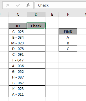
Here to find the category IDs which starts with either A , B or C, will be using the * (asterisk) wildcard in the formula. * (asterisk) wildcard finds any number of characters within lookup value.

Use the formula:

= SUM ( COUNTIF ( C3 , { «A*» , «B*» , «C*» } ) ) >0

Explanation:

COUNTIF function checks the value which matches with either of the pattern stated in the formula
Criteria is given in using * (asterisk) wildcard to look for value which has any number of characters.
COUNTIF function returns an array to the SUM function matching either of the values.
SUM function adds up all the values and checks whether the sum comes out to be greater than 0 or not.

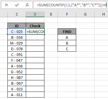
Here the range is given as array reference and pattern is given as cell reference. Press Enter to get the count.

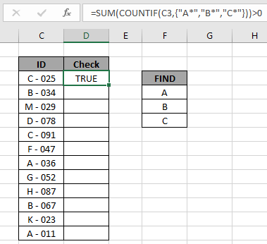
As you can see the formula returns TRUE for the value in C3 cell. Now copy the formula in other cells using the drag down option or using the shortcut key Ctrl + D as shown below.

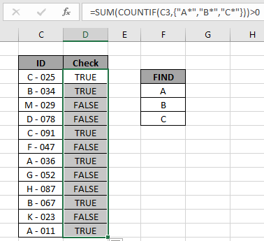
As you can see all the TRUE values indicate the cell value starts with either of mentioned pattern and all the FALSE values states there is the cell value starts with neither of mentioned pattern.

Verification:

You can check which values start with a specific pattern in range using the excel filter option. Apply the filter to the ID header and click the arrow button which appears. Follow the steps as shown below.

Steps:

Select the ID header cell. Apply filter using shortcut Ctrl + Shift + L
Click the arrow which appeared as a filter option.
Deselect (Select All) option.
Now search in search box using the * (asterisk) wildcard.
Type A* in the search box and select the required values or select the (Select All search result) option as shown in the above gif.
Do it for the other two values and get the count of all three which is equal to the result returned by the formula.

As you can see in the above gif all the 6 values which match the given pattern. This also means the formula works fine to get to check the values
Here are some observational notes shown below.

Notes:

The formula only works with numbers and text both
Operators like equals to ( = ), less than equal to ( <= ), greater than ( > ) or not equals to ( <> ) can be performed within function applied with numbers only.

Hope this article about how to Check values which start with either A , B or C using wildcards in Excel is explanatory. Find more articles on COUNTIF functions here. If you liked our blogs, share it with your fristarts on Facebook. And also you can follow us on Twitter and Facebook. We would love to hear from you, do let us know how we can improve, complement or innovate our work and make it better for you. Write us at info@exceltip.com
Related Articles

How to use the SUMPRODUCT function in Excel: Returns the SUM after multiplication of values in multiple arrays in excel.

COUNTIFS with Dynamic Criteria Range : Count cells depstartent on other cell values in Excel.

COUNTIFS Two Criteria Match : Count cells matching two different criteria on list in excel.

COUNTIFS With OR For Multiple Criteria : Count cells having multiple criteria match using the OR function.

The COUNTIFS Function in Excel : Count cells dependent on other cell values.

How to Use Countif in VBA in Microsoft Excel : Count cells using Visual Basic for Applications code.

How to use wildcards in excel : Count cells matching phrases using the wildcards in excel

Popular Articles

50 Excel Shortcut to Increase Your Productivity : Get faster at your task. These 50 shortcuts will make you work even faster on Excel.

How to use the VLOOKUP Function in Excel : This is one of the most used and popular functions of excel that is used to lookup value from different ranges and sheets.

How to use the COUNTIF function in Excel : Count values with conditions using this amazing function. You don’t need to filter your data to count specific values. Countif function is essential to prepare your dashboard.

How to Use SUMIF Function in Excel : This is another dashboard essential function. This helps you sum up values on specific conditions.

Источник

The logical IF statement in Excel is used for the recording of certain conditions. It compares the number and / or text, function, etc. of the formula when the values correspond to the set parameters, and then there is one record, when do not respond — another.

Logic functions — it is a very simple and effective tool that is often used in practice. Let us consider it in details by examples.

The syntax of the function «IF» with one condition

The operation syntax in Excel is the structure of the functions necessary for its operation data.

=IF(boolean;value_if_TRUE;value_if_FALSE)

Let us consider the function syntax:

Boolean – what the operator checks (text or numeric data cell).
Value_if_TRUE – what will appear in the cell when the text or numbers correspond to a predetermined condition (true).
Value_if_FALSE – what appears in the box when the text or the number does not meet the predetermined condition (false).

Example:

Logical IF functions.

The operator checks the A1 cell and compares it to 20. This is a «Boolean». When the contents of the column is more than 20, there is a true legend «greater 20». In the other case it’s «less or equal 20».

Attention! The words in the formula need to be quoted. For Excel to understand that you want to display text values.

Here is one more example. To gain admission to the exam, a group of students must successfully pass a test. The results are listed in a table with columns: a list of students, a credit, an exam.

list.

The statement IF should check not the digital data type but the text. Therefore, we prescribed in the formula В2= «done» We take the quotes for the program to recognize the text correctly.

The function IF in Excel with multiple conditions

Usually one condition for the logic function is not enough. If you need to consider several options for decision-making, spread operators’ IF into each other. Thus, we get several functions IF in Excel.

The syntax is as follows:

Here the operator checks the two parameters. If the first condition is true, the formula returns the first argument is the truth. False — the operator checks the second condition.

Examples of a few conditions of the function IF in Excel:

It’s a table for the analysis of the progress. The student received 5 points:

А – excellent;
В – above average or superior work;
C – satisfactory;
D – a passing grade;
E – completely unsatisfactory.

IF statement checks two conditions: the equality of value in the cells.

In this example, we have added a third condition, which implies the presence of another report card and «twos». The principle of the operator is the same.

Enhanced functionality with the help of the operators «AND» and «OR»

When you need to check out a few of the true conditions you use the function И. The point is: IF A = 1 AND A = 2 THEN meaning в ELSE meaning с.

OR function checks the condition 1 or condition 2. As soon as at least one condition is true, the result is true. The point is: IF A = 1 OR A = 2 THEN value B ELSE value C.

Functions AND & OR can check up to 30 conditions.

An example of using the operator AND:

It’s the example of using the logical operator OR.

How to compare data in two tables

Users often need to compare the two spreadsheets in an Excel to match. Examples of the «life»: compare the prices of goods in different bringing, to compare balances (accounting reports) in a few months, the progress of pupils (students) of different classes, in different quarters, etc.

To compare the two tables in Excel, you can use the COUNTIFS statement. Consider the order of application functions.

For example, consider the two tables with the specifications of various food processors. We planned allocation of color differences. This problem in Excel solves the conditional formatting.

Baseline data (tables, which will work with):

tables.

Select the first table. Conditional Formatting — create a rule — use a formula to determine the formatted cells:

In the formula bar write: = COUNTIFS (comparable range; first cell of first table)=0. Comparing range is in the second table.

To drive the formula into the range, just select it first cell and the last. «= 0» means the search for the exact command (not approximate) values.

Choose the format and establish what changes in the cell formula in compliance. It’s better to do a color fill.

Select the second table. Conditional Formatting — create a rule — use the formula. Use the same operator (COUNTIFS). For the second table formula:

Download all examples in Excel

Now it is easy to compare the characteristics of the data in the table.

Источник

08-03-2010, 04:01 PM

#1

Registered User

If Statement: �Starts With�

I�m having trouble writing an if statement that tests whether or not a cell starts with a certain value. Here�s the outcome I�m trying to produce:

If A1 starts with 1/, 2/, or 3/, then insert �Q1�
If A1 starts with 4/, 5/, or 6/, then insert �Q2�
If A1 starts with 7/, 8/, or 9/ then insert �Q3�
If A1 starts with 10/, 11/, or 12/, then insert �Q4�

How do I make one if statement that combines these stipulations?
08-03-2010, 04:21 PM

#2

Re: If Statement: �Starts With�

Is A1 a date? (not a text representation of a date). If so then you could use a formula like this

=»Q»&MATCH(MONTH(A1),{1,4,7,10})
08-03-2010, 04:24 PM

#3

Re: If Statement: �Starts With�

if its text
=CHOOSE(CEILING(LEFT(A1,(FIND(«/»,A1)-1))/3,1),»Q1″,»Q2″,»Q3″,»Q4″)
or just
=»Q»&CHOOSE(CEILING(LEFT(A1,(FIND(«/»,A1)-1))/3,1),1,2,3,4)
08-03-2010, 04:26 PM

#4

Registered User

Re: If Statement: �Starts With�

Hi dll,

It is indeed, and your formula works perfectly!! Thanks so much for your quick and accurate help
08-03-2010, 04:29 PM

#5

Registered User

Re: If Statement: �Starts With�

martin, yours also works flawlessly. thanks, guys!
08-11-2010, 01:47 PM

#6

Registered User

Re: If Statement: �Starts With�

If I want it to display the year as well (such as 2010 Q3), how would I modify the code?
08-11-2010, 02:00 PM

#7

Re: If Statement: �Starts With�

=year(a1) & » q» & match(month(a1),{1,4,7,10})

Entia non sunt multiplicanda sine necessitate
08-11-2010, 02:24 PM

#8

Registered User

Re: If Statement: �Starts With�