
In this example, the goal is to use a formula to check if a specific value exists in a range. The easiest way to do this is to use the COUNTIF function to count occurences of a value in a range, then use the count to create a final result.
COUNTIF function
The COUNTIF function counts cells that meet supplied criteria. The generic syntax looks like this:
=COUNTIF(range,criteria)Range is the range of cells to test, and criteria is a condition that should be tested. COUNTIF returns the number of cells in range that meet the condition defined by criteria. If no cells meet criteria, COUNTIF returns zero. In the example shown, we can use COUNTIF to count the values we are looking for like this
COUNTIF(data,E5)Once the named range data (B5:B16) and cell E5 have been evaluated, we have:
=COUNTIF(data,E5)
=COUNTIF(B5:B16,"Blue")
=1
COUNTIF returns 1 because «Blue» occurs in the range B5:B16 once. Next, we use the greater than operator (>) to run a simple test to force a TRUE or FALSE result:
=COUNTIF(data,B5)>0 // returns TRUE or FALSEBy itself, the formula above will return TRUE or FALSE. The last part of the problem is to return a «Yes» or «No» result. To handle this, we nest the formula above into the IF function like this:
=IF(COUNTIF(data,E5)>0,"Yes","No")This is the formula shown in the worksheet above. As the formula is copied down, COUNTIF returns a count of the value in column E. If the count is greater than zero, the IF function returns «Yes». If the count is zero, IF returns «No».
Slightly abbreviated
It is possible to shorten this formula slightly and get the same result like this:
=IF(COUNTIF(data,E5),"Yes","No")Here, we have remove the «>0» test. Instead, we simply return the count to IF as the logical_test. This works because Excel will treat any non-zero number as TRUE when the number is evaluated as a Boolean.
Testing for a partial match
To test a range to see if it contains a substring (a partial match), you can add a wildcard to the formula. For example, if you have a value to look for in cell C1, and you want to check the range A1:A100 for partial matches, you can configure COUNTIF to look for the value in C1 anywhere in a cell by concatenating asterisks on both sides:
=COUNTIF(A1:A100,"*"&C1&"*")>0
The asterisk (*) is a wildcard for one or more characters. By concatenating asterisks before and after the value in C1, the formula will count the text in C1 anywhere it appears in each cell of the range. To return «Yes» or «No», nest the formula inside the IF function as above.
An alternative formula using MATCH
As an alternative, you can use a formula that uses the MATCH function with the ISNUMBER function instead of COUNTIF:
=ISNUMBER(MATCH(value,range,0))
The MATCH function returns the position of a match (as a number) if found, and #N/A if not found. By wrapping MATCH inside ISNUMBER, the final result will be TRUE when MATCH finds a match and FALSE when MATCH returns #N/A.
Excel for Microsoft 365 Excel 2021 Excel 2019 Excel 2016 Excel 2013 Excel 2010 Excel 2007 More…Less
Let’s say you want to ensure that a column contains text, not numbers. Or, perhapsyou want to find all orders that correspond to a specific salesperson. If you have no concern for upper- or lowercase text, there are several ways to check if a cell contains text.
You can also use a filter to find text. For more information, see Filter data.
Find cells that contain text
Follow these steps to locate cells containing specific text:
-
Select the range of cells that you want to search.
To search the entire worksheet, click any cell.
-
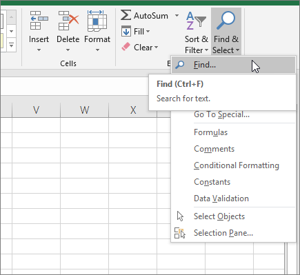
On the Home tab, in the Editing group, click Find & Select, and then click Find.

-
In the Find what box, enter the text—or numbers—that you need to find. Or, choose a recent search from the Find what drop-down box.
Note: You can use wildcard characters in your search criteria.
-
To specify a format for your search, click Format and make your selections in the Find Format popup window.
-
Click Options to further define your search. For example, you can search for all of the cells that contain the same kind of data, such as formulas.
In the Within box, you can select Sheet or Workbook to search a worksheet or an entire workbook.
-
Click Find All or Find Next.
Find All lists every occurrence of the item that you need to find, and allows you to make a cell active by selecting a specific occurrence. You can sort the results of a Find All search by clicking a header.
Note: To cancel a search in progress, press ESC.
Check if a cell has any text in it
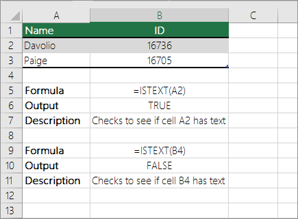
To do this task, use the ISTEXT function.
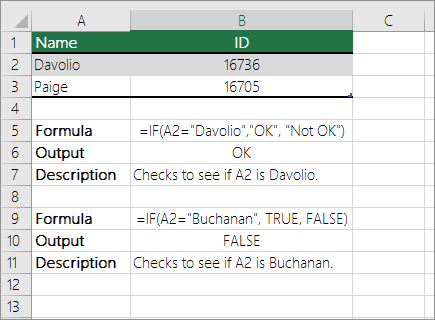
Check if a cell matches specific text
Use the IF function to return results for the condition that you specify.
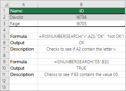
Check if part of a cell matches specific text
To do this task, use the IF, SEARCH, and ISNUMBER functions.
Note: The SEARCH function is case-insensitive.
Need more help?
Want more options?
Explore subscription benefits, browse training courses, learn how to secure your device, and more.
Communities help you ask and answer questions, give feedback, and hear from experts with rich knowledge.
Using an excel formula to search if all cells in a range read «True», if not, then show «False»
For example:
A      B     C     D
True  True  True   True
True  True  FALSE  True
I want a formula to read this range and show that in row 2, the was a «False» and since there are no falses in row 1 I want it to show «true.»
Can anyone help me with this?
![]()
asked Mar 5, 2014 at 15:37
![]()
2
You can just AND the results together if they are stored as TRUE / FALSE values:
=AND(A1:D2)
Or if stored as text, use an array formula — enter the below and press Ctrl+Shift+Enter instead of Enter.
=AND(EXACT(A1:D2,"TRUE"))
answered Jan 9, 2015 at 9:02
![]()
Simon DSimon D
4,1205 gold badges39 silver badges47 bronze badges
1
As it appears you have the values as text, and not the numeric True/False, then you can use either COUNTIF or SUMPRODUCT
=IF(SUMPRODUCT(--(A2:D2="False")),"False","True")
=IF(COUNTIF(A3:D3,"False*"),"False","True")
answered Mar 5, 2014 at 16:49
![]()
SeanCSeanC
15.6k5 gold badges45 silver badges65 bronze badges
2
=IF(COUNTIF(A1:D1,FALSE)>0,FALSE,TRUE)
(or you can specify any other range to look in)
answered Mar 5, 2014 at 15:45
![]()
ttaaoossuuuuttaaoossuuuu
7,7563 gold badges28 silver badges56 bronze badges
3
=COUNTIFS(1:1,FALSE)=0
This will return TRUE or FALSE (Looks for FALSE, if count isn’t 0 (all True) it will be false
answered Nov 1, 2019 at 21:15
![]()
EXPLANATION
This tutorial shows how to test if a range contains a specific value and return a specified value if the formula tests true or false, by using an Excel formula and VBA.
This tutorial provides one Excel method that can be applied to test if a range contains a specific value and return a specified value by using an Excel IF and COUNTIF functions. In this example, if the Excel COUNTIF function returns a value greater than 0, meaning the range has cells with a value of 500, the test is TRUE and the formula will return a «In Range» value. Alternatively, if the Excel COUNTIF function returns a value of of 0, meaning the range does not have cells with a value of 500, the test is FALSE and the formula will return a «Not in Range» value.
This tutorial provides one VBA method that can be applied to test if a range contains a specific value and return a specified value.
FORMULA
=IF(COUNTIF(range, value)>0, value_if_true, value_if_false)
ARGUMENTS
range: The range of cells you want to count from.
value: The value that is used to determine which of the cells should be counted, from a specified range, if the cells’ value is equal to this value.
value_if_true: Value to be returned if the range contains the specific value
value_if_false: Value to be returned if the range does not contains the specific value.
In this article, we will learn how to know if a range contains specific text or not.
For instance, you have a large list of data and you need to find the presence of substrings in a range using excel functions. For this article we will need to use 2 functions:
- SUMPRODUCT Function
- COUNTIF function with wildcard
SUMPRODUCT function is a mathematical function in Excel. It operates on multiple ranges. It multiplies the corresponding arrays and then adds them.
The COUNTIF function of excel just counts the number of cells with a specific condition in a given range.
A wildcard is a special character that lets you perform indefinite matching on text in your Excel formulas.
There are three wildcard characters in Excel
- Question mark (?)
- Asterisk (*)
- Tilde (~)
Generic formula:
Explanation:
- Here we need to apply the asterisk ( * ) with each substring. Asterisk ( * ) matches any number of characters when used.
- Then COUNTIF function takes argument of range & substrings with wildcard and counts the number of matched cells.
- SUMPRODUCT function takes the numbers returned by COUNTIF function and gets their SUM.
- The formula checks the outcome number with >0 and returns TRUE if the statement stands TRUE or else the formula returns FALSE.
Example:
Here we have data in range A2 : A7. we need to find the presence of Colors in Range using this formula.

Use the Formula:
= SUMPRODUCT ( COUNTIF ( range , «*» &Colors& «*» ) ) > 0
Explanation:
- Here the asterisk ( * ) is applied with each substring color. Asterisk ( * ) matches any number of characters when used.
- Then COUNTIF function takes argument of range & color with wildcard and counts the number of matched cells which comes out to be.
= SUMPRODUCT ( COUNTIF ( range , { *Red* ; «Green» ; «Blue» ))>0
- SUMPRODUCT function takes the numbers returned by COUNTIF function and gets their SUM which comes out here as.
=SUMPRODUCT ( { 1 ; 1 ; 1 } ) > 0
- The formula checks the outcome ( 3 ) number with >0 and returns TRUE.
Here the range is named range for A2 : A7 & Colors named for the substrings in C2 : C4.

As you can see in the above snapshot, the formula returns TRUE stats that the substring colors are found in the Range values.
Notes:
- The formula returns #VALUE! error if the argument to the function is numeric.
- The formula returns the wrong result if the formula syntax is not correct.
Hope this article about whether Range contains value using wildcards in Excel is explanatory. Find more articles on SUMPRODUCT functions here. Please share your query below in the comment box. We will assist you.
Related Articles
How to use the SUMPRODUCT function in excel
How to use the COUNTIF function in excel
How to use the WILDCARDS function in excel
How to Remove Text in Excel Starting From a Position
Validation of text entries
Create drop down list in excel with colour
Remove leading and trailing spaces from text in Excel
Popular Articles
Edit a dropdown list
Absolute reference in Excel
If with conditional formatting
If with wildcards
Vlookup by date
Join first and last name in excel
Count cells which match either A or B
Convert Inches To Feet and Inches in Excel 2016
50 Excel Shortcut to Increase Your Productivity